Interaction model for magnetic holes in a ferrofluid layer

Abstract

Nonmagnetic spheres confined in a ferrofluid layer (magnetic holes) present dipolar interactions when an external magnetic field is exerted. The interaction potential of a microsphere pair is derived analytically, with a precise care for the boundary conditions along the glass plates confining the system. Considering external fields consisting of a constant normal component and a high frequency rotating in-plane component, this interaction potential is averaged over time to exhibit the average interparticular forces acting when the imposed frequency exceeds the inverse of the viscous relaxation time of the system. The existence of an equilibrium configuration without contact between the particles is demonstrated for a whole range of exciting fields, and the equilibrium separation distance depending on the structure of the external field is established. The stability of the system under out-of-plane buckling is also studied. The dynamics of such a particle pair is simulated and validated by experiments.

I Introduction

The dynamic properties of so-called magnetic holes in ferrofluid layers has been the object of increasing interest over the past twenty years Skjeltorp (1983a); Helgesen and Skjeltorp (1991a); Skjeltorp (1983b, 1984a, 1984b, 1995, 1985); Skjeltorp and Helgesen (1991); Helgesen and Skjeltorp (1991b); Helgesen et al. (1990a, b); Helgesen and Skjeltorp (1991c); Miguel and Rubi (1996); Skjeltorp et al. (2001, 1999); Clausen et al. (1998a, b); Pieranski et al. (1996); Helgesen et al. (1988); Warner and Hornreich (1985); Davies et al. (1986); Sellers and Brenner (1989); Miguel and Rubi (1995). These systems consist of spherical non-magnetic particles in a carrier ferrofluid, whose size is order of magnitudes (1-100 $\mu m$) above the one of the magnetic particles (0.01$\mu m$) in suspension. The ferrofluid appears then as homogeneous at the scale of the large particles – holes –, and their effect on the magnetic field can be modelled as a dipolar perturbation, where the magnetic moment is opposite to the one of the displaced ferrofluid Skjeltorp (1983a). The system is generally confined between glass plates in quasi-two-dimensional layers, whose thickness slightly exceeds the diameter of the holes. The induced dipolar interactions give rise to a rich zoology of physical phenomena, such as crystallization of magnetic holes in constant or oscillating magnetic fields Skjeltorp (1983a); Helgesen and Skjeltorp (1991a); Skjeltorp (1983b, 1984a, 1984b), order-disorder transitions in those crystals Skjeltorp (1995, 1985); Skjeltorp and Helgesen (1991); Helgesen and Skjeltorp (1991b), or non-linear phenomena in the dynamics of those systems in low frequency oscillating fields Helgesen et al. (1990a, b); Helgesen and Skjeltorp (1991c); Miguel and Rubi (1996), commonly described using braid theory Skjeltorp et al. (2001, 1999); Clausen et al. (1998a, b); Pieranski et al. (1996).

The understanding of these systems is important in relation to industrial ferrofluid applications Chantrell and Wohlfart (1983); Rosensweig (1987), or for their potential use in biomedicine Ugelstad et al. (1993); Berge et al. (1989); Hayter et al. (1989). The dynamics of these phenomena can also be used indirectly to characterize the ferrofluid’s transport properties Rubi and Miguel (1993), as its viscosity. Eventually, the ability to shape the effective pair interaction potentials through the imposed external magnetic field, makes these system good candidates as large analog models to study phase transitions Skjeltorp (1987), aggregation phenomena Helgesen et al. (1988) or fracture phenomena in coupled granular/fluid systems.

Nonetheless, despite the theoretical studies on similar dual systems as ferromagnetic particles in a viscous fluid Laufer (1951); Newman and Yarbrough (1968), and the extensive experimental observations of these magnetic holes, there is a lack of theory describing this detailed effective pair interaction potentials. Notably, there has been no satisfying explanation so far for the existence of stable configurations of particles populations with finite separation distances in external fields consisting of a circular rotating inplane component and a constant normal one (reported in Helgesen and Skjeltorp (1991a)), or for the existence of out-of-plane buckled structures Skjeltorp and Helgesen (1991), and no theoretical framework for the influence of the ferrofluid layer thickness (separation of the embedding plates).

We will show here how the magnetic boundary conditions along the confining plates lead to rich effective interaction potentials rendering for those structures, rather than the qualitative magneto-hydrodynamic effects proposed in Helgesen and Skjeltorp (1991a). In particular, we give an explanation for the existence of a finite equilibrium separation between particles. Theoretical work has already been done along this line Warner and Hornreich (1985), but in a reduced case of constant normal field. The present study includes a circular high frequency oscillating field in addition. The potential derived should be an essential brick in all the applications mentioned above of the magnetic holes, and in general this type of contribution of the confining structure should be relevant to any quasi-2D colloidal system with a significant dielectric or magnetic permeability contrast between the fluid medium and the confining structure, as in Martinelli Kepler and Fraden (1994).

In this paper, we first describe the system under study and review briefly the basic modelling asumptions and standard theory. We next derive the instantaneous pair interaction potential with a precise care for the magnetic permeability contrast of the boundaries, and average it over the short oscillation periods to get the effective interactions. We turn then to the properties of the equilibrium configurations, sketch a simple dynamical theory and compare the theoretical and experimental results for the dynamics of a particle pair. Eventually, the three dimensional aspect of the ferrofluid layers is taken into account, to evaluate both gravity-induced corrections, and the stability of the system under out-of-plane buckling.

II System under study and basic assumptions

The system considered consists of two non-magnetic spheres inside a ferrofluid which is homogeneous at their scale, whose susceptibility and magnetic permeability are denoted respectively $\chi_{f}$ and $\mu_{f}=\mu_{0}(1+\chi_{f})$, where $\mu_{0}=4\pi\cdot 10^{-7}H.m^{-1}$. This ferrofuid is itself embedded between two glass plates considered as perfectly plane, parallel and nonmagnetic. The magnetic field anywhere between the glass plates is then decomposed between a uniform order zero component resulting from the outer imposed field, plus a perturbation due to the spheres. This perturbation is essentially dipolar: an isolated sphere in a field with a given uniform (constant) boundary value ${\bm{H}}$ at infinity provokes a purely dipolar perturbation outside it, generated by an effective dipole as shown in Figure 1:

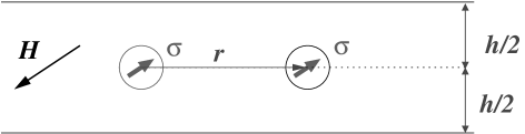
Figure 1: Pair of non magnetic particles in a ferrofluid layer and related effective dipolar moments due to the external magnetic field.

$${\bm{\sigma}} = -V\bar{\chi}{\bm{H}}$$ (1)

$$\bar{\chi} = \frac{\chi_{f}}{1+2\chi_{f}/3}$$ (2)

where $\bar{\chi}$ is an effective susceptibility including a demagnetization factor, i.e. whose precise form results when the boundary conditions for the magnetic field on the surface of the sphere are properly taken into account (see for example Warner and Hornreich (1985); Bleaney and Bleaney (1978)) – SI magnetic units are adopted throughout this whole paper, $V=\pi a^{3}/6$ and $a$ refer respectively to the volume and diameter of a sphere. This result justifys the name of magnetic holes used for those nonmagnetic spheres, and stays valid to leading order when a system more complicated than an isolated sphere is considered: it holds as soon as the external magnetic field ${\bm{H}}$ can be considered as uniform at the scale of a sphere, which will be assumed and commented further in section VI.2.

The average magnetic field inside the ferrofluid ${\bm{H}}$ itself is simply related to the external uniform magnetic field imposed outside the glass plates ${\bm{H}}^{e}$ through

$${\bm{H}}={\bm{H}}_{\|}^{e}+\frac{1}{1+\chi_{f}}{\bm{H}}_{\bot}^{e}$$ (3)

to fulfill the Boundary Conditions along the glass-ferrofluid planar interfaces – namely, ${\bm{H}}_{\|}^{e}={\bm{H}}_{\|}$ and ${\bm{B}}_{\perp}^{e}={\bm{B}}_{\perp}$ Bleaney and Bleaney (1978); Knoepfel (2000) – where the parallel and normal components are oriented relative to the glass plates.

The simplest model for a particle pair can be obtained first by neglecting the effect of the nonmagnetic boundaries: considering a couple of two such spheres of identical moments ${\bm{\sigma}}$ with a separation vector from center to center ${\bm{r}}$, the total interaction energy of the system is, after Bleaney and Bleaney Bleaney and Bleaney (1978),

$$U=\frac{\mu_{f}}{4\pi}{\bm{\sigma}}^{2}\left(\frac{1-3\cos^{2}\theta}{r^{3}}\right)$$ (4)

where $r=\left\|{\bm{r}}\right\|$ and $\theta=(\widehat{{\bm{r}};{\bm{\sigma}}})$ is the angle between the field and the separation vector.

We consider now external fields composed of a circular in-plane component oscillating at frequency $\nu$, superimposed to a constant normal one. At high enough frequency, the relative displacement of the particles during an oscillation period is negligible compared to its average value, and the time dependence of the separation vector can be decoupled in a slow and a fast varying mode, $\mathbf{r}(t)=\bar{\mathbf{r}}(t)+\delta\mathbf{r}(\bar{\mathbf{r}};t)$, with $\overline{\bf\delta r}=0$ and $\delta r\ll\bar{r}$ . Throughout the remainder of this paper , bold symbols refer to vectors, normal ones to their norm, and the upper bar refers to averaged quantities over oscillating time. Moreover, we will now use the additional constraint on ${\bm{r}}$ that it should be in-plane, under the effect of the glass plates over the microspheres which center them at positions equally separated from the top and bottom boundaries. The presence of the boundaries can indeed be represented by equivalent image dipoles outside the confining plates, as established in section III, which repel the dipole from the boundaries. This constraint will be adressed specifically in section VII, to show that this centering magnetic effect is valid in most work cases when no lateral confinement is exerted in the system – section VII.2 . The possible sink caused by gravity under the density contrast between the microspheres and the fluid is generally negligible – section VII.1. Thus, in the reference frame $(\hat{\bar{\mathbf{r}}};\hat{\mathbf{n}}\otimes\hat{\bar{\mathbf{r}}};\hat{\mathbf{n}})$ – where hats refer to unit vectors, instantaneous fields read

$${\bm{H}}=H(\cos\phi\sin\alpha;\sin\phi\sin\alpha,\cos\alpha)^{T}$$ (5)

with by definition

$$\text{cotan}\alpha=\beta=H_{\perp}/H_{\parallel}=H_{\perp}^{e}/(1+\chi_{f})H_{\parallel}^{e},$$ (6)

and $\phi=2\pi\nu t$. Thus, defining $\gamma=(\widehat{\bar{\mathbf{r}};{\bm{r}}})$, comes $\cos^{2}\theta=\cos^{2}(\phi-\gamma)\sin^{2}\alpha=\cos^{2}(\phi-\gamma)/(1+\beta^{2}),$ and

$$U({\bm{r}};\phi) = A\frac{a^{3}}{r^{3}}\left(2\beta^{2}-1-3\cos(2\phi-2\gamma)\right)$$ (7)

$$\text{with\, }A = \frac{\mu_{f}\sigma^{2}}{8\pi a^{3}(1+\beta^{2})}=\frac{\mu_{f}\pi a^{3}\chi^{2}H_{\parallel}^{2}}{288}.$$ (8)

Consider distant enough particles to prevent contact and significant hydrodynamic interactions during an oscillation period of the external field: the neglect of inertial terms allows to balance magnetic interaction forces and Stokes drag for both particles, which gives to leading order in $\delta r/\bar{r}$,

$$3\pi\eta a\cdot(\dot{\bar{\mathbf{r}}}+\delta\dot{\mathbf{r}})=-\nabla U({\bm{r}})$$ (9)

$$\!\!= \!\!\frac{3Aa^{3}}{\bar{r}^{4}}[(2\beta^{2}-1)\hat{\bar{\mathbf{r}}}+3\cos(2\phi)\hat{\bar{\mathbf{r}}}+2\sin(2\phi)\hat{\mathbf{n}}\otimes\hat{\bar{\mathbf{r}}}]$$

Neglecting inertial terms is easily justified since a large upper bound of Reynold’s number can be evaluated as being $Re=\rho xa^{2}\nu/\eta\leq 10^{-4}$ where $x=\delta r/a$ is the relative amplitude of the oscillations which will be shown straightforwardly to be typically below $10^{-2}$, for typical diameters $a=50\mu m$, ferrofluid’s viscosity $\eta=9\cdot 10^{-3}\,Pa.s$ and density $\rho=1000\,kg.m^{-3}$, and field oscillation frequency $\nu=100\,Hz$. Random thermal motion in the ferrofluid is essentially irrelevant at these size scales, as will be shown in section VI.2, justifying the use of deterministic dynamics instead of a Brownian one. The above Eqs. (7;9) establish that the slow motion $\bar{\mathbf{r}}$ is driven by an effective potential obtained through time-averaging over the oscillations of the field, i.e. simply using $\overline{\cos^{2}\phi}=1/2$ at fixed $\mathbf{r}=\bar{\mathbf{r}}$,

$$3\pi\eta a\dot{\bar{\mathbf{r}}} = -\nabla\overline{U}(\bar{\mathbf{r}})$$ (10)

$$\text{with\, }\overline{U}(\bar{\mathbf{r}}) = A\frac{a^{3}}{\bar{r}^{3}}(2\beta^{2}-1)$$ (11)

while small and quick elliptic oscillations are performed,

$$\delta\mathbf{r} = -\frac{\nu_{c}}{\nu}\frac{a^{5}}{\bar{r}^{5}}[3\sin(4\pi\nu t)\bar{\mathbf{r}}+2\cos(4\pi\nu t)\hat{\mathbf{n}}\otimes\bar{\mathbf{r}}]$$

$$\text{with\, }\nu_{c} = \frac{A}{4\pi^{2}\eta a^{3}}=\frac{\mu_{0}(1+\chi_{f})\bar{\chi}^{2}H_{\parallel}^{2}}{1152\pi\eta}$$

The relative magnitude of the fast oscillations $\delta r/\bar{r}=\nu_{c}a^{5}/\nu\bar{r}^{5}$ are indeed negligible as soon $\nu\gg\nu_{c}\simeq 0.1\,Hz$ for typical ferrofluids, $\chi_{f}=1.9$, $\overline{\chi}=0.84$, $\eta=9\cdot 10^{-3}Pa.s$ and fields $H_{\parallel}=14\,Oe$. $\nu_{c}$ , inverse of the viscous relaxation time of the system, is the critical frequency introduced in Helgesen et al. (1990b), above which a particle pair cannot anymore follow the direction of an external rotating field due to the fluid drag. In this paper, we study regimes where $\nu\geq 10\,Hz$, for which the relative variations of the separation vector are below 1%, and focus on the slow motion of the particles $\bar{\mathbf{r}}(t)$ driven by $\overline{U}(\bar{\mathbf{r}})$.

In this simple picture however, this average potential is a simple central one whose inverse cubic range reflects the dipole-dipole nature of the interactions, and in the absence of any characteristic length scale, this basic model predicts a very simple behavior for the particle pair: depending on the ratio $\beta$ of the normal over the in-plane field, either the two particles will repel each other without end if $\beta>\beta_{c}=1/\sqrt{2}$, or they will attract each other when $\beta<\beta_{c}$, until the magnetic forces are balanced by contact forces or very short-range hydrodynamic forces sensitive when particles almost touch – when $(r-a)/a$ gets insignificant: this theory is obviously insufficient to render for the finite equilibrium separation distance, sometimes at a few diameters, which is experimentally observed for a whole range of imposed fields Helgesen and Skjeltorp (1991a). A proper treatment of the boundary conditions of the system along the glass plates, introducing the plate separation as an extra length scale to the problem, will in the next section be shown to remedy this problem.

III Effect of the boundaries on the instantaneous interactions

The boundaries between the ferrofluid and the embedding glass plates are supposed to be perfectly plane. The two microspheres are supposed perfectly centered between the glass plates, and the perturbation of the magnetic field due to the presence of those spheres is modeled as a perturbation due to two identical point-like dipoles ${\bm{\sigma}}=-\overline{\chi}V{\bm{H}}$ located at the center of the spheres. To fulfill the magnetic boundary conditions – i.e. the continuity of $H_{\|}$ and $B_{\perp}$– along the plates, a direct use of the image method (e.g. Weber Weber (1950)) shows that this magnetic perturbation between the plates is equal to the field emitted, in an unbounded uniform medium of susceptibility $\chi_{f}$, by an infinite series of dipoles: the two original ones, at locations defined as $\bm{0}$ and ${\bm{x}}$, plus an infinite set of images for each of them corresponding to the mirror symmetry across the plane boundaries of the sources and all of the successive images. A magnification factor

$$\kappa=\frac{\mu_{f}-\mu_{0}}{\mu_{f}+\mu_{0}}=\frac{\chi_{f}}{\chi_{f}+2}$$ (12)

multiplies the amplitude of the dipolar moments at each symmetry operation, i.e. explicitly defined by the following conditions:

For any dipole source ${\bm{\sigma}}$ at position ${\bm{r}}_{0}$, with $\bm{h}$ the normal separation vector between the plates, an infinite set of dipolar images indexed by $l\in\mathbb{Z}$ is defined by their locations and moments – see figure 2:

$${\bm{r}}_{l}-{\bm{r}}_{0} = l{\bm{h}}$$ (13)

$${\bm{\sigma}}_{l_{\|}} = \kappa^{|l|}{\bm{\sigma}}_{\|}$$ (14)

$${\bm{\sigma}}_{l_{\perp}} = \kappa^{|l|}(-1)^{\left|l\right|}{\bm{\sigma}}_{\perp}$$ (15)

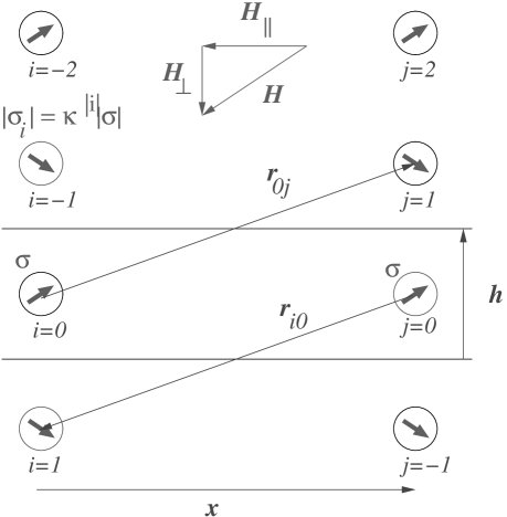
Figure 2: Image dipoles representing the Boundary Conditions.

The total interaction energy of such a system – where all dipoles do not have anymore the same moment – is (Bleaney and Bleaney Bleaney and Bleaney (1978))

$$U=\frac{\mu_{f}}{8\pi}\sum_{b\neq c}\frac{1}{r_{bc}^{3}}\left[{\bm{\sigma}}_{b}\!\cdot\!{\bm{\sigma}}_{c}-\frac{3\left({\bm{\sigma}}_{b}\!\cdot\!{\bm{r}}_{bc}\right)\left({\bm{\sigma}}_{c}\!\cdot\!{\bm{r}}_{bc}\right)}{{\bm{r}}_{bc}^{2}}\right]$$ (16)

where the sum on the $b$ index runs over the two source dipoles, and the one over the $c$ index runs over the whole set of sources and image dipoles – as seen in the preceding section, separation vectors can be considered as constant over the quick variations of ${\bm{\sigma}}$, and the upper bars over ${\bm{r}}$ are implicit for the remainder.

We will then use the following straightforward geometrical equalities resulting from Eqs. (1,6,13-15) : if the $c$ index represents the $l$-th image of the source $b$, then

$$\frac{{\bm{\sigma}}_{b}\!\cdot\!{\bm{\sigma}}_{c}}{\kappa^{|l|}\sigma^{2}} = \frac{1+(-1)^{l}\beta^{2}}{1+\beta^{2}}$$ (17)

$$\frac{\left({\bm{\sigma}}_{b}\!\cdot\!{\bm{r}}_{bc}\right)\left({\bm{\sigma}}_{c}\!\cdot\!{\bm{r}}_{bc}\right)}{\kappa^{|l|}\sigma^{2}{\bm{r}}_{bc}^{2}} = \frac{\beta^{2}(-1)^{l}}{1+\beta^{2}}$$ (18)

$$r_{bc} = |l|h.$$ (19)

If on contrary $c$ represents the $l$-th image of one source – as indexed in Figure 2 – , and $b$ the other source, then

$$\frac{{\bm{\sigma}}_{b}\!\cdot\!{\bm{\sigma}}_{c}}{\kappa^{|l|}\sigma^{2}}\!\! \!\!=\!\! \!\!\frac{1+(-1)^{l}\beta^{2}}{1+\beta^{2}}$$ (20)

$$\frac{\left({\bm{\sigma}}_{b}\!\!\cdot\!{\bm{r}}_{bc}\right)\!\!\left({\bm{\sigma}}_{c}\!\!\cdot\!{\bm{r}}_{bc}\right)}{\kappa^{|l|}\sigma^{2}{\bm{r}}_{bc}^{2}}\!\! \!\!=\!\! \!\!\frac{\left(y\cos\phi\!+\!\!\beta(-1)^{l}l\right)\!\!\left(y\cos\phi\!+\!\!\beta l\right)}{\left(1+\beta^{2}\right)\left(y^{2}+l^{2}\right)}$$ (21)

$$r_{bc}\!\! \!\!=\!\! \!\!\sqrt{x^{2}+l^{2}h^{2}}$$ (22)

where

$$y=\frac{x}{h}$$ (23)

is the ratio of the particle in-plane separation distance to the plate separation. Introducing those equalities in Eq. (16) we get:

$$\!\!\!\!\!\frac{U}{2Aa^{3}} = \frac{I_{0}^{so}}{x^{3}}+\sum_{l\in\mathbb{Z}^{*}}\kappa^{|l|}\left[\frac{I_{l}^{ss}}{|l|^{3}h^{3}}+\frac{I_{l}^{so}}{(x^{2}+l^{2}h^{2})^{3/2}}\right]$$ (24)

$$\!\!\!\!\!I_{l}^{ss} = 1-2(-1)^{|l|}\beta^{2}$$ (25)

$$\!\!\!\!\!I_{l}^{so} = \left[1+(-1)^{|l|}\beta^{2}\right.$$ (26)

$$\left.-3\frac{\left(y\cos\phi\!+\!\!\beta(-1)^{|l|}l\right)\!\!\left(y\cos\phi\!+\!\!\beta l\right)}{\left(y^{2}+l^{2}\right)}\right]$$

where $A$ is the constant defined in Eq. (8). The first term, denoted by $I_{0}^{ss}$, is the direct interaction between the two sources, the next one $I_{l}^{ss}$ corresponds to the interactions between the sources and their own images, and finally the term $I_{l}^{so}$ corresponds to the cross-interactions between a source and the images of the other one.

IV Time-averaged effective interactions

IV.1 Derivation of the potential

The ${\bm{H}}$-fields consist of a perfectly circular in-plane component ${\bm{H}}_{\|}=H_{\|}(\cos\phi\hat{{\bm{r}}}+\sin\phi\hat{{\bm{n}}}\wedge\hat{{\bm{r}}})$, and a normal component ${\bm{H}}_{\perp}$ which is maintained constant. During an oscillation of the in-plane field, the only significantly varying quantity in Eq. (16) is the angle $\phi$, with once again $\overline{\cos^{2}\phi}=1/2$.

The term $I_{l}^{ss}$, e.g. the interactions between a source and its own images, naturally does not depend on the in-plane separation vector ${\bm{x}}$, and produces no net in-plane force. It is worthwhile to note that this would however not be the case for any non-plane interfaces, giving the possibility to quench any geometrical property of the roughness of the interfaces in this potential. In the current hypothesis of purely planar plates, this interaction term is only responsible for a normal centering force, as will be established in section VII.2. For the present purpose where the microspheres are constrained on the half-plane between the plates, the in-plane forces are the only relevant ones, and this term is simply discarded in the following.

The remaining terms produce through time-average the interaction energy

$$\overline{U}({\bm{x}})=A\frac{d^{3}}{h^{3}}u\left(\frac{x}{h}\right)$$ (27)

with $A$ the constant defined in Eq. (8), and a dimensionless term

$$u(y)\!\! \!\!=\!\! \!\!(2\beta^{2}-1)y^{-3}$$

$$+4\sum_{l=1}^{+\infty}\kappa^{l}\left(\frac{1+(-1)^{l}\beta^{2}}{(y^{2}+l^{2})^{3/2}}-\frac{3}{2}\frac{y^{2}+2(-1)^{l}l^{2}\beta^{2}}{(y^{2}+l^{2})^{5/2}}\right)$$

The first term reduces to the expression of the first-order theory of Eq. (11), which is a test of self-consistency, since an infinite medium would be equivalent to the absence of permeability contrast along the plates, $\kappa=0$. The following ones render for the interactions between a source and the images of the other one. Due to the cylindrical symmetry of the problem with a purely circular in-plane field, this interaction is isotropic: the dependence on the separation vector ${\bm{x}}$ enters only through its norm $x=hy$.

IV.2 Properties of the isotropic interactions

The introduction of those images is responsible for possible finite separation equilibrium distances for a whole range of $\beta$ characterizing the imposed magnetic field, as is illustrated in Figure 3:

(a) Purely attractive, $\beta<\beta_{m}$

(b) Metastable, $\beta_{m}<\beta<\beta_{c}$

(c) Stable,  $\beta_{c}<\beta<\beta_{u}$

(d) Purely repulsive, $\beta_{u}<\beta$

Figure 3: Possible types of the interactions depending on $\beta$.

In this example, a typical susceptibility $\chi_{f}=1.9$ was considered for the ferrofluid, i.e. $\kappa=0.49$. The four potentials $u(y)$ represented correspond respectively to $\beta=0.4,\,0.58,\,0.8,\,2.1$. They were obtained by truncating the sums in Eq. (IV.1) to order $l=10$, which corresponds to a relative error lower than $10^{-3}$ in $u$ for any $y$.

The general typology of those potentials can be classified in four cases as will be demonstrated in the next section, separated by three particular values of $\beta$, referred to as $\beta_{m}$, $\beta_{c}$ and $\beta_{u}$ – which depend only on the susceptibility $\chi_{f}$:

• (a) For $\beta<\beta_{m}$ , $u$ is a monotonically increasing function, and the magnetic forces are purely attractive, thus leading any pair of spheres to contact.

• (b) For $\beta_{m}<\beta<\beta_{c}$, $u$ presents a short-range attractive core, and presents both a maximum – an instable equilibrium point – at some distance $y_{i}$, typically slightly below $1$, and a minimum – a stable equibrium point – at a greater distance $y_{s}$, usually above $1$.
  Two locally stable equilibrium configurations are possible in principle, depending on the ratio $y_{a}=a/h$ of the particle diameter to the plate separation, and of the initial particle separation $y_{\text{init}}$: if $y_{\text{init}}>y_{i}$, the particles should end up at the equilibrium separation $y_{s}$, which since $y_{s}>1>y_{a}$ corresponds to an equilibrium configuration without contact between the particles. If on contrary $y_{\text{init}}<y_{i}$, the particles should attract each other and end up in contact at $y_{a}$. Since any separation $y<y_{a}$ is forbidden due to contact forces, this second case is only possible when $y_{a}<y_{i}$, i.e. when the ratio of plate separation over particle diameter is sufficiently big. In that case, if the thermal fluctuations are large enough to let the particles go over the energy maximum at $y_{i}$ with a significant probability over the observation time, only one of the two possible equilibrium configurations will be thermodynamically stable, and the other one will be only metastable. The selection of stability / metastability between the two is determinated by the comparison of $u(y_{a})$ and $u(y_{s})$.

• (c) For $\beta_{c}<\beta<\beta_{u}$, $u$ presents only a global minimum, which thus corresponds to a stable equilibrium separation distance $y_{s}$. Since generally $y_{s}>1>y_{a}$, this equilibrium configuration corresponds to a finite separation distance $hy_{s}-a>0$.

• (d) For $\beta_{u}<\beta$, $u$ is monotonically decreasing, and the time averaged magnetic forces are purely repulsive at any separation.

V equilibrium separation distance as function of the applied field

The separation equilibrium distance $y_{eq}$ – which is stable or not – correspond to the extrema of the potential, and can be obtained in principle by solving

$$\frac{du}{dy}(y_{eq})=0.$$ (29)

$y_{eq}$ corresponds to $y_{s}$ or $y_{i}$ defined in section IV.2, according to the sign of $d^{2}u/dy^{2}$. Derivating Eq. (IV.1) with respect to the scaled separation $y$, leads straightforwardly to

$$\frac{y^{4}}{3}\!\frac{du}{dy}\! \!=\! \!(1-2\beta^{2})\!-\!2\sum_{l=1}^{+\infty}\!\kappa^{l}\lambda_{l}(y)\!(-1+2(-1)^{l}\beta^{2})$$ (30)

$$\lambda_{l}(y)\! \!=\! \!\frac{(y^{2}-4l^{2})y^{5}}{(y^{2}+l^{2})^{7/2}}$$ (31)

The Eq. (30) above is the sum of a term independent of $\beta$, plus another proportional to $\beta^{2}$. The constant term can be shown to be positive, and the prefactor of $\beta^{2}$ strictly negative, for any possible $(y,\kappa)$ – i.e. any $y>0,0\leq\kappa<1$. Thus, $du/dy(y,\beta)$ is a monotonic decreasing function of $\beta^{2}$, equal to zero when

$$\beta_{0}(y)=\sqrt{\frac{1+2\sum_{l=1}^{+\infty}\kappa^{l}\lambda_{l}(y)}{2+4\sum_{l=1}^{+\infty}(-1)^{l}\kappa^{l}\lambda_{l}(y)}}$$ (32)

Thus, for a given field configuration $\beta$, and separation $y$, pair interactions are attractive, i.e. $du/dy>0$, if $\beta<\beta_{0}(y)$, and conversely if $\beta>\beta_{0}(y)$. A numerical study of the above function, for any $\kappa$, shows that $\beta_{0}(y)$ is monotonically decreasing from $\beta_{c}=1/\sqrt{2}$ to a finite positive minimum $\beta_{m}(\kappa)$, between $y=0$ to $y_{m}(\kappa)$, and next monotonically increasing up to a finite limit $\beta_{u}(\kappa)>\beta_{c}$ between $y_{m}(\kappa)$ and $y\rightarrow+\infty$.

These considerations allow to obtain by a direct graphical inversion of $\beta_{0}(y)$, the possible roots $y_{s}(\beta)$ and $y_{i}(\beta)$ for which the interaction forces are zero at a given field geometry $\beta$, as shown in Figure 4 which is obtained for the particular case $\chi_{f}=1.9,$ i.e. $\kappa=0.49$.

Figure 4: Equilibrium separation of a pair as function of the applied field

This nonlinear dependence of the equilibrium separation $y_{s}(\beta)$ seems more complex than observed in earlier experiments by Helgesen and Skjeltorp Helgesen and Skjeltorp (1991a). This apparent discrepancy will be resolved in the next section, which is centered on finite time results.

Identifying the three parameters $\beta_{m},\beta_{c},\beta_{u}$ identified above as

$$\beta_{c} = \beta_{0}(y=0)$$ (33)

$$\beta_{m} = \min_{y}\beta_{0}(y)=\beta_{0}(y_{m})$$ (34)

$$\beta_{u} = \lim_{y\rightarrow+\infty}\beta_{0}(y),$$ (35)

these arguments prove that the pair effective potentials belong to one of the four types described in the previous section:

(a) If $\beta<\beta_{m}$, the potential is purely attractive at any separation.

(b) If $\beta_{m}<\beta<\beta_{c}$, there are two roots to Eq. (29), denoted $y_{i}(\beta)$ and $y_{s}(\beta)$: the potential is attractive below $y_{i}$ or above $y_{s}$, and repulsive between both.

(c) If $\beta_{c}<\beta<\beta_{u}$, the potential presents a single minimum at $y_{s}(\beta)$.

(d) If $\beta>\beta_{u}$. the potential is purely repulsive and there is no equilibrium separation.

The definition of $\beta_{u}$ above – Eq. (35) – shows also clearly that $\lim_{\beta\rightarrow\beta_{u}^{-}}(y_{s})=+\infty$: in principle, it should be possible to drive a pair of microspheres in an equilibrium configuration with any desirable separation distance. Naturally, since the magnetic interactions decay rapidly with distance, thermal processes or any kind of external perturbation in the fluid flow, or default in the planarity of the plates, will be predominent at large separations, where this theory will become inapplicable.

The dependence of $\beta_{c},\beta_{u},\beta_{m}$ on the susceptibility of the ferrofluid (through the parameter $\kappa$) is as follows: Replacing $\lambda_{l}(0)=0$ in Eq. (32) shows that

$$\beta_{c}=1/\sqrt{2}$$ (36)

independently of $\kappa$. Similarly, since $\lim_{y\rightarrow+\infty}\lambda_{l}(y)=1$, $\beta_{u}$ is easily summed as

$$\beta_{u} = \frac{1}{\sqrt{2}}\sqrt{\frac{1+2\sum_{l=1}^{+\infty}\kappa^{l}}{1+2\sum_{l=1}^{+\infty}(-\kappa)^{l}}}$$ (37)

$$= \frac{1}{\sqrt{2}}\frac{1+\kappa}{1-\kappa}$$

A numerical study of $\beta_{m}$ shows that it decreases monotonically with $\kappa$, down to zero when $\kappa\rightarrow 1$.

This shows that the range of $\beta$ over which stable equilibrium distances exist is larger when the susceptibility of the ferrofluid is important ($\kappa$ increases with $\chi_{f}$, $\beta_{m}$ and $\beta_{u}$ are respectively decreasing and increasing with $\kappa$), up to the limiting case of an infinitly susceptible ferrofluid $\kappa\rightarrow 1$ ($\chi_{f}\gg 1$), for which $\beta_{m}\rightarrow 0,\,\beta_{u}\rightarrow+\infty$, and there is a finite stable equilibrium separation for any ratio $\beta$.

The other limiting case $\kappa\rightarrow 0$ is obtained directly by discarding the sums in Eq. (32) - their convergence to $0$ in that limit for any $y$ is straightforward -. This shows that $\lim_{\kappa\rightarrow 0}\beta_{m}=\lim_{\kappa\rightarrow 0}\beta_{u}=\beta_{c}=1/\sqrt{2}$: without any permeability contrast along the glass plates, no images are felt and the first-order theory is recovered - the interactions are simply purely attractive when $\beta<\beta_{c}$, and purely repulsive when $\beta>\beta_{c}$, with the stable regimes $\beta\in[\beta_{m},\beta_{u}]$ disappearing.

An overall picture of $y_{eq}(\beta)$ for different values of $\kappa$ distributed regularly between $0$ and $0.9$ is given in figure (5).

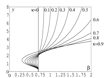
Figure 5: Equilibrium separation distances as function of the applied field, for various ferrofluids.

The sums in Eq. (32) have been truncated to order 10, which results in an accuracy better than 1% for the displayed function $\beta_{0}(y)$ – functions $\lambda_{l}(y)$ defined in Eq. (31) can be bounded by $|\lambda_{l}(y)|<1/(y^{2}+l^{2})^{3/2}$, so that $\left|\sum_{l=N}^{+\infty}\kappa^{l}\lambda_{l}(y)\right|<\sum_{l=N}^{+\infty}\kappa^{l}\left|\lambda_{l}(y)\right|<\kappa^{N}/(1-\kappa)N^{3}$, and similarly for $\left|\sum_{l=N}^{+\infty}(-\kappa)^{l}\lambda_{l}(y)\right|$. Thus, neglecting terms from order $N=11$ in the sums, for any $\kappa<0.9$, results in a relative error on $\beta_{0}(y)$, smaller than $0.9^{11}/(1-0.9)11^{3}\simeq 0.0023$.

VI Finite-time theory and experiments

VI.1 Simple time-dependent theory

The preceding section was centered on equilibrium properties of this system, but the relaxation time to reach equilibrium amounts to hours or days in certain configurations, as will be shown here. In order to compare efficiently theoretical and experimental data, we have therefore concentrated on the slow dynamics of this system, starting from hole pairs in contact under the effect of a purely in-plane field $\beta=0$, through the following scheme: neglecting once again the inertial terms, Stokes drag and magnetic interactions are balanced to obtain

$$3\pi\eta a\frac{dx}{dt}=-\frac{d}{dx}\overline{U}(x)$$ (38)

where the effective potential includes the images due to the boundaries, Eq. (27). The viscosity $\eta$ above is renormalized to take into account hydrodynamic interactions with the confining plates, as will be detailed further.

In dimensionless units, this equation leads to

$$T\frac{dy}{dt^{\prime}} = -\frac{d}{dy}u(y)$$ (39)

$$\text{with\, }T = \frac{864\eta}{\mu_{0}(1+\chi_{f})\bar{\chi}^{2}H_{\parallel}^{2}}\frac{h^{5}}{d^{5}}$$ (40)

and $y(t^{\prime})=x/h,$ $t^{\prime}=t/T$, and $u(y)$ the potential defined in Eq. (IV.1). The characteristic time above lies typically around $30\,s$ to $5\,min$ at usual working parameters, as will be shown in the next section, and moreover the potential wells can be pretty flat, thus producing often metastable situations that last from minutes to hours (the driving force close to equilibrium position is proportional to the distance to it, times the second derivative of the potential in the well, and $u^{\prime\prime}(y_{s})\rightarrow 0$ when $\beta\rightarrow\beta_{u}^{-}$).

Starting from a pair configuration in contact, and setting at time $0$ the field parameters ($\beta$ ratio and magnitude $H_{\parallel}$) to a constant value, the time $t^{\prime}(y)$ to reach a given separation will be directly obtained through numerical integration of the differential Eq. (39):

$$t^{\prime}(y)=-T\int_{z=a/h}^{y}dz/u^{\prime}(z).$$ (41)

An inverse representation of the above is plotted for a ferrofluid of susceptibility $\chi_{f}=1.9$. In Figure 6, the solid thin line represents $y(t^{\prime})$ at fixed $\beta=0.8$, and in Figure 7, the dashed lines represent $y(\beta)$ for four characteristic times $t^{\prime}=.25,\,1,\,4,\,16$, slowly converging to equilibrium separation $y_{s}(\beta)$, plotted as a solid line.

To compare this with experiments, the fine tuning of the time dependence requires a refined analysis of the hydrodynamic interactions in the above: since experiments are carried out in cells of width $h$ comparable with the diameter $a$ of the embedded holes – typically $h/a$ lies between 1.1 and 2 –, a strong hydrodynamic coupling with the confining plates is present. Considering that both particles sit at a fixed fraction $z$ of the plate separation relative to the central position (nonzero $z$ can be obtained in principle between horizontal plates due to the density contrast between the particles and ferrofluid), these interactions are represented according to Faucheux and Libchaber (1994), by a normalization of the Stokes drag as

$$\eta/\eta_{0}=f[a/(h+2zh)]+f[a/(h-2zh)]-1$$ (42)

with $\eta_{0}$ the naked viscosity of the carrier ferrofluid, and

$$f(x)=\left(1-\frac{9x}{16}+\frac{x^{3}}{8}-\frac{45x^{4}}{256}-\frac{x^{5}}{16}\right)^{-1}+O(x^{6}).$$ (43)

Two experimental cases will be considered here, where $h/a=1.4;\,z\simeq 0$ and $h/a=2,\,z\simeq 0.14$, corresponding respectively to $\eta/\eta_{0}\simeq 2.6$ and $2.4$. This is consistent with Faucheux and Libchaber’s measures for a confined brownian motion Faucheux and Libchaber (1994) , and with an experimental value $\eta/\eta_{0}\simeq 2.4$, that we measured in the $h/a=1.4$ case by placing $50\,\mu m$ diameter particles between $70\,\mu m$ distant plates set up in vertical position, without any magnetic field, and by recording the motion of a single particle under the effect of buoyancy forces. The density of the ferrofluid was $\rho_{f}=1.24$, the one of the polystyrene particles $\rho_{p}\simeq 1$. This value is slightly below the theoretical $\eta/\eta_{0}\simeq 2.6$, which is consistent with the effect of the brownian motion of the particle along the normal direction, as analyzed in Faucheux and Libchaber (1994). We have chosen to use $\eta/\eta_{0}=2.5$ in the following.

Hydrodynamic interactions between both particles were neglected, which should be a relatively poor approximation for particles close to contact, but become reasonable at separations $x/h>2$ where most of the time is spent to achieve equilibrium at relatively large separations, and is therefore the most important one in the present context. The typical magnitude of this error can be roughly estimated through the analyzes performed by Dufresne et al. or Grier and Behrens Davies et al. (1986); Grier and Behrens (2001) for a close context: they derived for two particles of diameter $a$, separated by $x$ and at a distance $h/2$ from a single plate, the hydrodynamic corrections to the mobility to first order in $x/a$ and $x/h$. Considering for simplicity a double contribution for two plates relatively to Eq. (13) in Davies et al. (1986), contributions due to the particle-particle interactions, become for $h/a=1.4;\,x/h>2$, less than 30% of the one due to the plates – term $9x/16$ in Eq. (43).

We neglect also the rotational degrees of freedom of the ferrofluid itself, which can lead to the rotation of the nonmagnetic spheres, and induce another type hydrodynamic interactions between pairs of spheres: in ferrofluids submitted to circular magnetic fields, the rotation of the magnetite particles induces asymmetric stresses in the fluid, which leads to a counter-rotation of the magnetic holes Helgesen and Skjeltorp (1991a); Miguel and Rubi (1995). The mismatch between this rotational motion of the magnetic holes and the one of the magnetites could in principle induce a vortex in the fluid flow around each of the holes, which would lead to a net hydrodynamic torque over close pairs of holes. Nonetheless, with the ferrofluid and field frequency regime used here (<100 Hz), this rotational motion of the holes is so slow that it is hardly detectable with the field frequency used ($\nu_{f}<100Hz$). Experimentally, with a similar ferrofluid (kerosene-based, $\chi=0.8$), the hole’s frequency was bounded by $\nu_{s}<0.01Hz$. This rotational motion was described theoretically in detail by Miguel and Rubi Miguel and Rubi (1995). Through this theory, for the ferrofluid and field frequencies used here, the frequency of the magnetic holes will straightforwardly be shown to be lower than $\nu_{s}<0.05Hz$. This justifies for the present study the neglect of these rotation-induced hydrodynamic interactions. These interactions would in any case lead to a purely rotational motion of the hole pair, decoupled from the purely central forces induced by the magnetic interactions studied here. Experimentally, some very slow rotational motion of the hole pairs was indeed occasionally observed when the particles were close (non periodic, angular velocity always lower than 0.001 Hz), but no systematic trend for its direction or velocity was noted, i.e. this effect was beyond the experimental error.

To obtain the theoretical estimate of the hole’s frequency above, the Langevin parameter of the ferrofluid, defined Miguel and Rubi (1995) as $\mu=m_{0}H/k_{B}T$ where $m_{0}$ is the magnetic moment of the magnetites, is derived from the saturation magnetization of the ferrofluid and its susceptibility Larson (1999) as $\mu=3H/\chi M_{\text{sat}}.$ For the ferrofluid used, $\chi=1.9$, $M_{\text{sat}}=200G$, $H=14$ Oe, and $\mu=0.26$. This enables to express the ratio of the hole’s frequency over the field’s one, as Miguel and Rubi (1995)

$$\nu_{s}/\nu_{f}=-\Phi(\mu-\text{tanh}\mu)/(\mu+\text{tanh}\mu)=-0.00041$$ (44)

where $\Phi=-0.036$ is the magnetite volume fraction of the ferrofluid. For the regime $\nu_{f}<100Hz$ where the experiments are carried, the spheres frequency is thus below $\nu_{s}=0.041Hz$.

VI.2 Experimental results and scaling

We used pairs of $a=50\,\mu m$ diameter neutral polystyrene spheres of density $\rho_{p}=1$, designed according to Ugelstad’s technique Ugelstad and Mork (1980), and ferrofluids of susceptibility $\chi_{f}=1.9$, density $\rho_{f}=1.24$ and viscosity $\eta_{0}=0.009\,Pa.s$ Fer , confined in horizontal cells of thickness $70\,\mu m$ or $100\,\mu m$ and width of order centimeters. The thickness of the cell was obtained by confining plates by quenching a few 70 $\mu m$ diameter spheres between the two plates clamped together (these spacers where typically half a centimeter distant from each other). The oscillating inplane and constant normal field were generated by external coils, with a typical magnitude $H_{\parallel}=H_{0}=14.2\,Oe$, with frequencies from 10 to 100 $H\!z$. Magnitudes and phase of the field are accurate up to 1%, which also corresponds to the degree of homogeneity of the in and out-of-plane fields throughout the entire cell. The direction of the constant field varies slightly along the cell, with a maximum $3^{\circ}$ misalignment from the direction normal to the confining planes (these accuracies for the homogeneity and misalignment of the field were obtained directly by considering the geometry of the Helmholtz coils generating the field, whose characteristic extent is 10 cm, together with a .5 mm accuracy for the position of the cell inside them). The in-plane motion of the particles was recorded using a microscope, and a camera linked to a numerical data analysis setup. The entire experimental setup is described, for example, in Ref. Helgesen and Skjeltorp (1991c). The samples were prepared with a pure inplane field to bring the particles in contact, after that the inplane field was maintained constant and the normal field was set to a constant $H_{\perp}^{e}=(1+\chi_{f})\beta H_{\parallel}$. The normal field required typically a few seconds to stabilize. Separation between the particles were then recorded every $10\,s$, for $30\,min$. The concentration of the spheres in the entire sample was such as the nearest sphere or spacer would sit at least 20 diameters apart from the observed pair, which was sufficiently dilute not to influnce the motion of the observed pair.

VI.2.1 Time-dependent result at fixed field geometry and discussion.

The scaled separation as function of time is shown in Figure 6, for five experiments carried out at $\beta=0.8$, i.e. for the potential represented in Figure 3 (c), which presents a single minimum at $y_{s}(0.8)=2.35$. Four experiments were carried out in a $h=70\,\mu m$ thick cell, two of them at identical field amplitudes $H_{\parallel}=H_{0}=14.2\,Oe$, and two other at $H_{\parallel}=0.7\,H_{0};\,0.5\,H_{0}$. The last experiment was carried out in a $h=100\,\mu m$ thick cell, with an inplane field $H_{0}$.

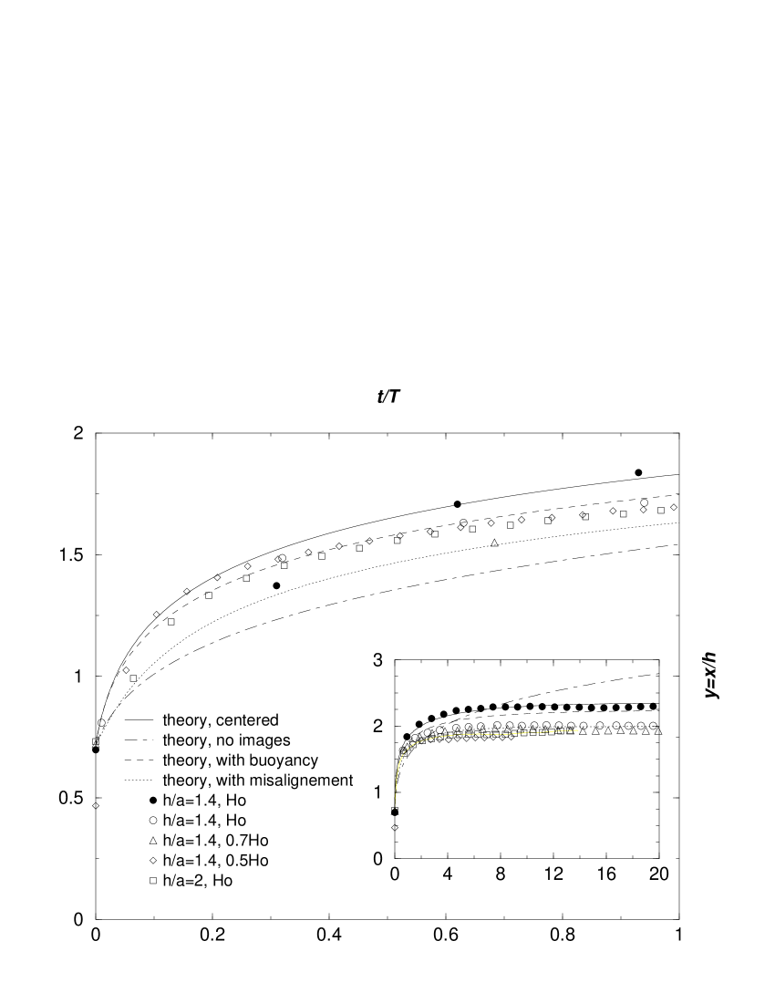
Figure 6: Scaled separation as function of time for various field magnitudes and plate separations, for $\beta=H_{\perp}/H_{\parallel}=0.8$. The inset represents the same data for longer times.

These parameters corresponded respectively to characteristic times evaluated using Eq. (40) as $T=32\,s,\,63\,s,\,129s,\,192s$.

Comparison with the theory.

The large part of the figure represents the short time evolution $t<T$ (typically the first minutes), the encapsulated part shows longer time (typically 30 min). Every data point (separated by 10 s) was used for the early regime, one point out of 2 to 12 depending on the experiment for the later one. At shorter times, the scaled data collapse reasonably well on the theoretical curve obtained from the theory sketched so far – solid line. The only two main outliers (first filled circle and triangle, $t=10s$) presumably corresponded to a weaker normal field in the first few seconds, until it stabilized. For illustration, the first-order theory neglecting the magnetic confinement leads to the dot-dashed curve, obtained using Eq. (41) with a bare potential retaining only the source-source term. This too simple theory clearly differs from data both at short and large times.

Corrections due to buoyancy.

A third dashed theoretical curve was plotted, corresponding to a slightly refined calculation of the interaction potential, where buoyancy forces due to the density contrast between ferrofluid and particles led to a shift $z$ of the particle pairs from the central mid-plane of the cell. The relative displacement $z/h$ due to this gravitational correction is evaluated in section VII.1 as $15\%$ in the weakest fields $0.5\,H_{0},\,h/a=1.4$ case, and in the thicker layer $H_{0},\,h/a=2$ case, whereas it should remain around $6\%$ for the thiner cells, higher field $H_{0}$ case. The extended potential to take this lateral shift into account is also derived in section VII.1, and the dashed curve corresponds to this potential at a fixed shift $z/h=14\%$, which is the maximum possible in the thin cells, since it would correspond to contact of the particles with one of the plates, coinciding with $z/h=(1-a/h)/2$ at $h/a=1.4$. Considering this correction, one would expect the diamond and squares to follow the dashed line, the circles to be close to the solid line, and the triangle to sit in between. This is indeed approximately the case at shorter times for the diamonds and rectangles, and the filled circles fit well with the centered theory, both at short and long times. Nonetheless, it is worth noticing that the open circles, collapse rather with the lower field experiments than with the filled circles, another experiment carried with identical parameters. This gives an estimate of the reproducibility of these experiments, corresponding roughly to a relative experimental error bar of $10\%$ for the separation at a given time, estimated between open and filled circle cases. The gravity-induced correction discussed above is of order $5\%$ for the separation as function of the dimensionless time, and the effect of this shift on the magnetic interactions can therefore hardly be distinghished from experimental dispersion in terms of separation. Still, the renormalization of the time due to hydrodynamic interactions with the plates would lead in the thick cell case $h/a=2$, to $\eta/\eta_{0}\simeq 1.2$ if the particles were considered as centered $z/h=0$, instead of the value $\eta/\eta_{0}=2.5$ that we used and corresponded to the predicted shift in that case, $h/a=2,\,z/h=0.15$. This gravity-induced correction is then clearly sensible for the hydrodynamic corrections, if not so much on the magnetic interactions, since the above incorrect viscosity $\eta$ would correspond to dividing $T$ by $2$, which would double the abscissas of the square data points and drive them way out of the theory and rest of the data. This shows qualitatively that this shift was indeed present in cases $h/a=2,\,H_{0}$, and $h/a=1.4,\,0.5\,H_{0}$, and that particles sat close to or in contact with a plate in this last case.

Corrections due to experimental error on the field directions.

The fourth dotted curve represents the theoretical effect of a misalignment of angle $\alpha=2.5^{\circ}$ between the constant field and the normal direction. A direct generalization of sections II to IV to such configurations with a slightly tilted constant field, shows that the time averaged potential is still of the form in Eqs. (25,26), with a modified parameter

$$\beta^{\prime} = \frac{{\bm{H}}_{\perp}^{e}}{(1+\chi_{f})({\bm{H}}_{\parallel}+\sqrt{2}\sin(\alpha)\cos(\theta){\bm{H}}_{\perp}^{e})}$$ (45)

$$\simeq \beta-\sqrt{2}(1+\chi_{f})\beta^{2}\sin(\alpha)\cos(\theta),$$

where $\theta$ is the angle between the projection of the constant field over the plane and the separation vector. This modified interaction potential leads to a torque tending to align the particle pair with the direction $\theta=0$, and a radial interaction force corresponding to a modified $\beta^{\prime}$ in $[\beta-\sqrt{2}(1+\chi_{f})\beta^{2}\sin(\alpha);\beta]$, $\beta^{\prime}$ decreasing with time towards the lower limit as the pair aligns with the inplane constant component of the field. The dotted curve corresponds to this lower limit for a possible misalignment $\alpha=2.5^{\circ}$, which is evaluated from the above as $\beta^{\prime}=0.68$.

For the longer time period shown in the encapsulated part of figure 6, an apparent equilibrium position was reached in each experiment after typically $6\,T$ – no more than a 1% relative motion was noticed later when the experiments were several hours. This equilibrium separation corresponds theoretically to the equilibrium one studied in the previous section, $y_{s}(0.8)=2.35$. The high field and thin cell experiment (filled circles) agree well (within 2%) with the theory with a purely normal field (solid line), but discrepancies between solid line and experiments are noticeable at longer times for the four other experiments. A comparison of the data with the dotted line shows that a misalignment of order $2.5^{\circ}$ between constant field and normal direction is sufficient to explain these discrepancies: in these experiments, the particle pairs started at a relatively large angle $\theta$ from the inplane component of the constant field, which is why the unmodified theory and experimental data are close for short times. At longer times, the particle pairs aligned with the direction $\theta=0$, and the modified theory $\beta^{\prime}=0.68$ agrees well with the data. An initial rotation of the particle pair and subsequent locking of this direction in a particular one was indeed observed in these experiments.

Brownian motion in the ferrofluid can be proved to be entirely negligible for the relatively large particles and field we worked with, its relative magnitude compared to magnetic interaction energy being $kT/\min\overline{U}\leq kT/[A(d^{3}/h^{3})\min u]\simeq 10^{-4}/\min u\leq 5\cdot 10^{-3}$ for the fields, particles and plate separations considered here.

VI.2.2 Scaled time-dependent results at various field geometries

Experiments were carried out with inplane field magnitudes $H_{0}$, and normal fields jumping at initial time from $0$ to $\beta(1+\chi_{f})H_{0}$ with various $\beta$ from 0 to 3.5. This was done for $a=50\,\mu m$ diameter particles, and plates separation $h=70\,\mu m$ and $100\,\mu m$. The results, scaled separation as function of $\beta$, at four values of the scaled time, are shown in Figure 7(a) for the thinner cell. The error bars correspond to a possible misalignment $\alpha=2.5^{\circ}$ between the constant field and the normal direction: they represent the limits $[\beta-\sqrt{2}(1+\chi_{f})\beta^{2}\sin(\alpha);\beta]$ for the effective $\beta^{\prime}$ parameter as explained in the previous section.

(a) h/d=1.4, with a potential $2.5^{\circ}$ misalignement between constant field and normal direction

(b) comparison between two plate separations

Figure 7: Separation as function of time and $\beta$ for various field configurations, times and cell sizes: merged data and theory.

For the “c”-regime $\beta>\beta_{c}=1/\sqrt{2}\sim 0.7$, theory and experiment agree well for any of the tested field parameters and times.

The solid line represents the theoretical equilibrium value, studied in section V. This is reached within typically $16\,T$ (8 min for $h/a=1.4$, $H_{\parallel}=H_{0}$) for $\beta\leq 1$, or longer time at higher $\beta$. This is the main reason why the upwards curvature of the theoretical solid curve at larger values of $\beta$ is not observed in experimental data, which correspond to finite times, and for which other types of perturbations always enter the picture at very large times and distances.

In Figure 7(b), we present the results of experiments carried out at two different plate separations, as function of time and value of $\beta$. The error bars have been omitted for readability, and the experimental points represented correspond to a constant field supposed purely normal (i.e. the abcissas are the upper limit of the error bars in Figure 7(a)). The experiments carried out in thicker cells, corresponding to weaker magnetic interaction forces, are more sensitive any perturbations. The relative data collapse for both plate separations at $0.25\,T$ and $T$ when $\beta>\beta_{c}$ nonetheless show that the separations in this regime scale with plate separation, and not with particle diameter. Apart from the misalignment of the constant field with the normal direction, a possible source for these perturbations is as follows: when the particles come close to equilibrium, inplane magnetic forces tend to zero, and the particle motion becomes more sensitive to any interactions with the local environment (confining plates) – this being of course even more the case for weaker fields or larger $h/a$: there seems to be a pinning (friction) of the particles to an absolute plate position at large times. The physical origin of this pinning is possibly due to roughness of the plates (especially when particles are almost in contact), which can quench the particles through the magnetic perturbation due to this roughness (the repulsion effect of a dipole by its images would make a particle sit preferably in positions of larger plate separation), or alternatively when particles are almost in contact with the plates can result in an inplane component of the hydrodynamic coupling or contact forces responding to buoyancy forces. Instead of plate roughness, the same type of qualitative effects could be due to small impurities in the ferrofluids, starting to stick to the plates or particles at large times, when the chemical surfactant layers around large particles and possible impurities, break apart in some points.

For the regime $\beta<\beta_{c}$, the simple theory presented here would predict that particles stay always in contact at $y=a/d=0.5$ or $0.71$ for $\beta<\beta_{m}\sim 0.55$, and for $\beta_{m}<\beta<\beta_{c}$ would either stay in contact if $a/h<y_{i}(\beta)$ or go to the secondary minimum $y_{s}(\beta)$ if $y_{i}(\beta)<a/h$ (the separation between first and second case happening at $\beta=0.61$ for $a/h=1/1.4,$ and $\beta=0.67$ for $a/h=1/2$). Particles seem indeed to be in contact for $\beta\leq 0.2$, but start to separate significantly well before $\beta_{m}$. We note also that this separation seems grossly to be proportional to the particle diameter when $\beta\leq 0.3$, where some finite separation can already be observed – ordinates of opened and filled symbols are multiple of each other through a factor $100/70$ – and proportional to plate separation in the regime $\beta_{m}<\beta<\beta_{c}$. This shows that an extra physical effect that was not taken into account here, generated repulsive forces, whose range is finite but scales with the particle diameter. This effect suppresses then the short range attraction in the regime $\beta_{m}<\beta<\beta_{c}$, so that the particle jump directly to $y_{s}(\beta)$, which is always a stable minimum and not a metastable one. For $\beta<\beta_{m}$, this extra effect starts to separate the particles in proportion to particle diameter. The physical origin of this short range repulsion should not be the particle-particle hydrodynamic interactions, which should slow down the relative motion rather than result in a net repulsion – see Grier and Behrens (2001); Dufresne et al. (2000) –. A probable candidate for this repulsion is rather the magnetic effect of the finite size of the spheres, particularly sensible when particles are close to contact: even if an isolated nonmagnetic sphere generates a purely dipolar perturbation when it is isolated in a homogeneous susceptible medium, this dipolar perturbation does not fulfill the boundary conditions along the surface of another magnetic sphere, sufficiently close of the first one to feel the heterogeneity of the perturbation at the scale of its diameter, which is naturally the case at a finite separation/diameter ratio. To model this short range repulsion requires accounting for the magnetic perturbation generated by this non pointlike character of close enough spherical particles. Though this can be performed by a simple image method for pairs of discs in 2D, one can show that this does not extend to pairs of spheres in 3D, and the proper mathematical description of this perturbation requires the use of a series of spherical harmonics, which was not performed in the present study. To conclude this discussion, we note that this correction seems to be negligible at separations exceeding the sphere diameter $x/a>2$, as shows the agreement between experimental data and the present theory when $\beta>\beta_{m}$.

Finally, we note that the present results are not contradictory with similar experiments carried out in Helgesen and Skjeltorp (1991a) with a slightly different ferrofluid, plate separation and particle size, where it was reported that the equilibrium particle separation is approximately linear in $\beta$ once particles have started to separate: for example, this is also the case with the present ferrofluid, in the particular case $h/a=1.4$ in the regime $0.3<\beta<1$ – see the filled triangles or theoretical curve in Figure 7(a). This linear property is however shown here to be a mere coincidence, for this does not hold in the same $\beta$ regime for $h/a=2$, or for any $h/a$ when $\beta>1$, where $y_{s}(\beta)$ is curved upwards, and any result $y(\beta,t)$ observed at a given finite time $t$ is curved downwards.

VII generalization to quasi2D systems

VII.1 Gravity induced corrections

Although the effect of the dipolar images in the confining plates tends to center particles at a mid-plane position, the density contrast between the ferrofluid and particles tends to drive the particle out of it for large enough particles. An estimation of this effect can be obtained by considering for each particle, the sole effect of its own images, plus buoyancy forces – for the simple estimation we look at here, we will neglect the coupling between one source and the images of the other. Extending the analysis performed in sections III and IV.1 to a single dipole lying at a vertical distance $z$ from the center between two horizontal plates, comes directly

$$\overline{U}^{\text{shifted}}(z) = A\frac{a^{3}}{h^{3}}u^{\text{shifted}}(\frac{z}{h})$$ (46)

$$u^{\text{shifted}}(s) = \sum_{l\in\mathbb{Z}^{*}}\kappa^{\left|l\right|}\frac{1-2(-1)^{l}\beta^{2}}{\left|l-(1+(-1)^{l+1})s\right|^{3}}$$ (47)

This potential can be shown to be always centering for any value of $\beta$, i.e. to have a single minimum in $s=0$, and to diverge to infinity at $s=\pm 0.5$ – plate contact for very small particles. Equilibrium between gravity forces and magnetic interactions between the dipole and its images leads to

$$\frac{d\overline{U}^{\text{shifted}}}{dz} = V(\rho_{g}-\rho_{f})$$ (48)

$$\text{i.e.\, }\frac{du}{ds} = \frac{48(\rho_{g}-\rho_{f})gh}{\mu_{f}\bar{\chi}^{2}H_{\parallel}^{2}}\frac{h^{3}}{d^{3}}$$ (49)

For small separations (i.e, small particles or strong enough fields), a Taylor expansion to first order around the plates’ center gives

$$\frac{du}{ds} = 96\cdot C(\kappa)\cdot(1+2\beta^{2})\cdot|s|$$ (50)

$$C(\kappa) = \sum_{n\in N}\kappa^{2n+1}/(2n+1)^{5}$$ (51)

which is valid up to 25% for $s<0.1$. Thus, the displacement looked for can be evaluated as

$$s=z/a=\frac{(\rho_{g}-\rho_{f})gh}{2C(\kappa)(1+2\beta^{2})\mu_{f}\bar{\chi}^{2}H_{\parallel}^{2}}\frac{h^{3}}{a^{3}}$$ (52)

when this quantity does not exceed $0.1$, or directly using Eqs. (49,50) otherwise. For the ferrofluid and particles we used, this led respectively for $h=70\,\mu m,\,H_{\parallel}=H_{0};0.7\,H_{0}$ or $0.5\,H_{0}$, and $h=100\,\mu m;\,H_{\parallel}=H_{0}$, to $s=0.06,\,0.10,\,0.15$ and $0.15$ .

The magnetic interaction potentials were unaffected up to 1% in the $s=0.06$ vertical shift case, and the dashed curve in Figure 6 was obtained by considering particles at a fixed $s=0.14$ out-of-midplane shift, using a generalized potential obtained for a configuration sketched in Figure 8 through an extension of the method used in sections III and IV.1,

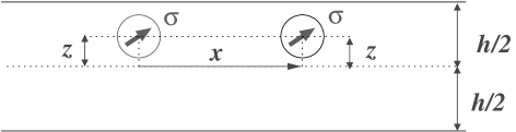
Figure 8: Shifted hole pairs considered.

as

$$u_{s}^{\text{pair}}(y)=(2\beta^{2}-1)y^{-3}$$

$$+4\sum_{l=1}^{+\infty}\kappa^{l}\left(\frac{1+(-1)^{l}\beta^{2}}{(y^{2}+m_{s}(l)^{2})^{3/2}}-\frac{3}{2}\frac{y^{2}+2(-1)^{l}m_{s}(l)^{2}\beta^{2}}{(y^{2}+m_{s}(l)^{2})^{5/2}}\right)$$

$$m_{s}(l)=l+s\cdot\left[1+(-1)^{l}\right]$$ (54)

This $s=0.14$ value was picked to represent the magnetic effect of a shift sufficient to bring particles in contact with the plates in the $h/a=1.4;\,0.5\,H_{0}$ case. To an accuracy of 1%, the results for $s=0.15$ were very close to this case, the ones for $s=0.06$ very close to pure inplane situations, and the situation $s=0.10$ fell roughly halfway between both, and were therefore omitted from Figure 6 for readability.

VII.2 Stability of the plane solutions and buckled configurations

When particles are sufficiently small or fields sufficiently high, the preceding section establishes that the confining plates have an effective repulsive effect on an isolated particle, which is therefore centered on midplane. In the case of a pair of particles, the interactions between one source and the images of the other one might nonetheless modify that picture, and make the plane solutions described in this paper unstable as have been observed in some experiments. Neglecting gravity, we will here generalize the interaction potential, to configurations where particle pairs are allowed to tilt on both sides of the midplane, i.e. where both are displaced by the same distance $z$ on both sides of it – cf Figure 9. We consider only symmetric situations, due to the symmetry of the problem under parity in the absence of gravitational forces.

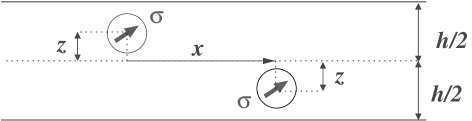
Figure 9: Tilted hole pairs considered.

The effective interaction potential is obtained similarly to the plane one, and comes as $\overline{U}(x,z)=A(a^{3}/h^{3})\cdot u(x/h,z/h)$ where

$$u(y,s)\!\! \!\!=\!\! \!\!2\!\sum_{l=-\infty}^{+\infty}\!\kappa^{|l|}\!\left(\frac{1+(-1)^{l}\beta^{2}}{(y^{2}+(l+p_{l}s))^{2})^{3/2}}-\right.$$

$$\qquad\qquad\quad\left.\frac{3}{2}\frac{y^{2}+2(-1)^{l}(l+p_{l}s)^{2}\beta^{2}}{(y^{2}+(l+p_{l}s)^{2})^{5/2}}\right)$$

$$\!\!+2\!\sum_{l\in\mathbb{Z}^{*}}\!\kappa^{|l|}\!(1\!-\!2(-1)^{l}\!\beta^{2})\!\left(\frac{1}{|l+(2-p_{l})s|^{3}}\!-\!\frac{1}{|l|^{3}}\!\!\right)$$

$$p_{l} = 1+(-1)^{l}$$ (56)

which reduces to the previous in-plane solution, Eq. (IV.1), when $s=0$. Contour plots of this pair potential are displayed in Figure 10, for the ferrofluid used here, $\chi_{f}=1.9$, and the four types of potentials – $\beta$ values are identical to the ones adopted in section IV.2. Black and white represent respectively $u=-0.2$ and $0.5$ in subfigures (a) and (b), $u=-0.2$ and $1$ in (c) and (d), and the grey level linear in $u$ in between. Out-of-plane values represented cover the whole possible range $0\leq s\leq 0.5$ in (c) and (d), and are restricted to 10% from the midplane in (a) and (b).

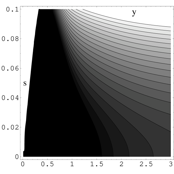
(a) $\beta<\beta_{m}$

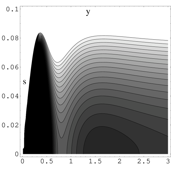
(b) $\beta_{m}<\beta<\beta_{c}$

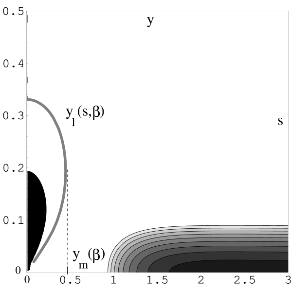
(c) $\beta_{c}<\beta<\beta_{u}$

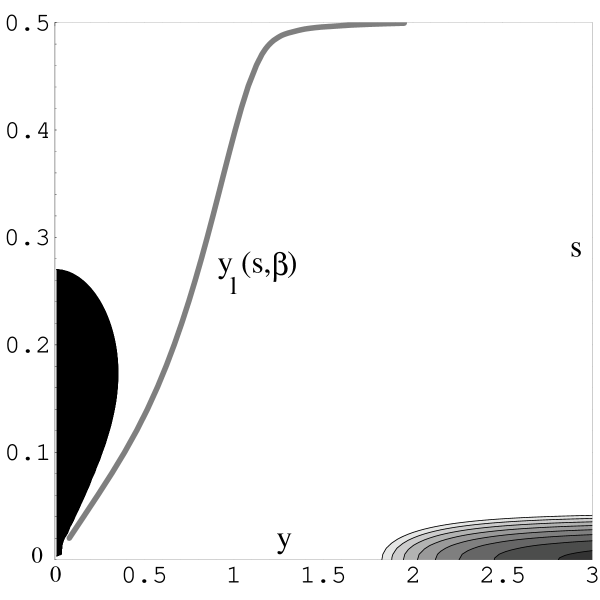
(d) $\beta_{u}<\beta$

Figure 10: Contour plots of the interaction potential as function of inplane separation y and tilt coordinate s.

The inplane configurations correspond to the bottom axis of those graphs.

Inplane solutions are in principle locally stable if $\partial^{2}u/\partial s^{2}(y,0)>0$, otherwise particle pairs will tend to tilt. For both first cases, $\beta<\beta_{c}$, we note that $\partial^{2}u/\partial s^{2}>0$ for any possible $(y,s)$, and any tilt is restored by the magnetic image effect: the plane configurations are indeed stable. As soon as $\beta>\beta_{c}$, besides the minima $(y,s)=(y_{s},0)$ or $(+\infty,0)$ in c or d case, another local minimum appears at a certain $(0,s_{e}(\beta))$: particles can be stable at a finite distance on top of each other – the pair tends to align with the large normal field –, or if they are close enough to be attracted by this potential minimum but too large ($a>s_{e}(\beta)$ and $a>h/2$), contact forces between them and with the confining plates will attract them to a “buckled” configuration where both particles are in contact with each other, and with one different plate each. Note that $0<s_{e}(\beta)<0.5$, i.e. very small particles $a\ll h$ at this second minimum would sit on top of each other, neither in contact between them nor with the plates. The criterion to determine whether particles are attracted by the inplane solution, or the buckled configurations, is to determine whether the present $(y,s)$ lie in the basin of attraction of one minimum or the other. Both basins of attraction are separated by a ridge of the potential, on which $u$ decreases under the effect of any perturbation of $(y,s)$ apart from the ones directed exactly along its gradient. This boundary between both basins of attraction, noted $y_{l}(s,\beta)$ was determined numerically and plotted as the grey solid line in Figure 10 (c) and (d). We note that the whole axis $(y,0)$ lies in the basin of attraction of the plane minimum, so any particle pair starting with no tilt should end up so. However, at short enough distances $y$ in a c-field, or at any inplane distance in a d-field, certain configurations with a finite tilt are attracted by the normal-aligned pair minimum, and will end up in a buckled contact configuration or normal-aligned pair. We have determined for every $\beta$, the maximum $y_{m}(\beta)=\max_{s}y_{l}(s,\beta)$: for a given $\beta$, when $y>y_{m}(\beta)$ any tilted configuration will be attracted by the inplane solution, whereas for certain finite tilts at close enough $y<y_{m}(\beta),$ the pairs will be attracted towards buckled in-contact configurations. The function $y_{m}(\beta)$ is displayed as the dashed curve in Figure 11 – the solid curve in a reminder of the equilibrium inplane distances $y_{s}(\beta),y_{i}(\beta)$ determined in section V. The function $y_{m}(\beta)$ diverges when $\beta\rightarrow\beta_{u}^{-}$, illustrating the fact that in any d-type field, configurations with out-of-plane tilts $s$ close to $0.5$, i.e. both particle centers almost along the plates (for small enough particles) will be attracted by the normal-aligned pair mode.

Figure 11: Stability limits of the in-plane configurations.

This effect is believed to be responsible for the lattices of buckled chains of particles in contact observed in Skjeltorp and Helgesen (1991). These were observed in pure normal fields ($\beta=+\infty)$, and the non-trivial character of the lattices, being hexagonal or square instead of triangular lattices characteristic of attractive interactions at any range, can be qualitatively explained by frustration effects: neighboring particles tend to sit in top-down contact configurations, but top-top or down-down configurations are repulsive – cf shifted potential developed in the previous section – and therefore lattices with noneven number of particles along the loops, as the triangular one, are disfavored in comparison with those involving even numbers in loops, as the square or hexagonal ones.

Eventually, the local stability of a plane configuration was investigated in fields of c- or d-type: the second derivative $\partial^{2}u/\partial s^{2}$ is positive at $s=0$ for large enough distances, and small out-of-plane tilts will be restored by magnetic interactions, but below a certain $y<y_{p}(\beta)$, $\partial^{2}u/\partial s^{2}(y,s=0)<0$, and the inplane solution will be locally instable. However, the preceding established that this out-of-plane character will be transient, since this case will still be attracted at long times by the inplane solution. This upper limit $y_{p}(\beta)$ below which inplane configurations will go to a transient out-of-plane regime, was determined numerically for any $\beta$ and plotted as the dash-dot curve in Figure 11.

VIII Conclusions

For pairs of magnetic holes in ferrofluid layers of finite thickness, exposed to fast oscillating conic magnetic fields, we have established the effective interaction potential driving their slow motion. The importance of the magnetic permeability contrast between ferrofluid and confining plates on these interaction was demonstrated, and the resulting pair potential analytically derived. This allowed the classification of those interaction potentials into four types, two of which present a secondary minimum at a finite distance. A simple finite time theory for these non-Brownian microspheres, including the hydrodynamic interactions of the holes with the confining plates, was directly compared and confirmed by experimental results, through data collapse of the scaled separation as function of scaled time, for various plate separations and field magnitudes. The relaxation time of these systems to reach equilibrium when there is any, was typically a few minutes or above. Eventually, we generalized the study to full three dimensions in the layer thickness, and studied the stability of the in-plane configurations. This established that although inplane configurations are stable at small normal fields, or at large ones and sufficient particle separation, hole pairs can be attracted by another stable configuration of tilted pairs of particles with contact between them and contact with one plate each.

This simple theory renders for so far unexplained observed configurations of magnetic holes, namely 2D lattices with finite separation, or buckled lattices of tilted pairs of particles. In principle, the effect described here in detail should be important in any colloidal system confined in a layer with significant magnetic permeability or dielectric contrast between the fluid and confining structure.

The ability to tune the equilibrium distance at will through the ratio of the normal over in-plane magnitude of the external field, makes this magnetic hole system a good candidate for various applications, as the manipulation of large molecules using the magnetic holes, for example proteins which would be fixed to one or several holes coated with antigens, the determination of the transport properties of a ferrofluid, or as analog model of systems implying discrete particles of tunable interactions and hydrodynamic coupling to the carrier fluid. The effective pair interactions derived here should be a fundamental brick of any such applications.

References

- Skjeltorp (1983a) A.T. Skjeltorp, Phys. Rev. Lett. 51, 2306 (1983a).
- Helgesen and Skjeltorp (1991a) G. Helgesen and A.T. Skjeltorp, J. Magn. Magn. Mater. 97, 25 (1991a).
- Skjeltorp (1983b) A.T. Skjeltorp, J. Magn. Magn. Mater. 37, 253 (1983b).
- Skjeltorp (1984a) A.T. Skjeltorp, J. Appl. Phys. 55, 2587 (1984a).
- Skjeltorp (1984b) A.T. Skjeltorp, Physica B & C 127, 411 (1984b).
- Skjeltorp (1995) A.T. Skjeltorp, Physica A 213, 30 (1995).
- Skjeltorp (1985) A.T. Skjeltorp, J. Appl. Phys. 57, 3285 (1985).
- Skjeltorp and Helgesen (1991) A.T. Skjeltorp and G. Helgesen, Physica A 176, 37 (1991).
- Helgesen and Skjeltorp (1991b) G. Helgesen and A.T. Skjeltorp, Physica A 170, 488 (1991b).
- Helgesen et al. (1990a) G. Helgesen, P. Pieranski, and A.T. Skjeltorp, Phys. Rev. Lett. 64, 1425 (1990a).
- Helgesen et al. (1990b) G. Helgesen, P. Pieranski, and A.T. Skjeltorp, Phys. Rev. A 42, 7271 (1990b).
- Helgesen and Skjeltorp (1991c) G. Helgesen and A.T. Skjeltorp, J. Appl. Phys. 69, 8277 (1991c).
- Miguel and Rubi (1996) M.C. Miguel and J.M. Rubi, Physica A 231, 288 (1996).
- Skjeltorp et al. (2001) A.T. Skjeltorp, S. Clausen, and G. Helgesen, J. Magn. Magn. Mater. 226, 534 (2001).
- Skjeltorp et al. (1999) A.T. Skjeltorp, S. Clausen, and G. Helgesen, Physica A 274, 267 (1999).
- Clausen et al. (1998a) S. Clausen, G. Helgesen, and A.T. Skjeltorp, Int. J. Bifurcat. Chaos 8, 1383 (1998a).
- Clausen et al. (1998b) S. Clausen, G. Helgesen, and A.T. Skjeltorp, Phys. Rev. E 58, 4229 (1998b).
- Pieranski et al. (1996) P. Pieranski, S. Clausen, G. Helgesen, and A.T. Skjeltorp, Phys. Rev. Lett. 77, 1620 (1996).
- Helgesen et al. (1988) G. Helgesen, A.T. Skjeltorp, P.M. Mors, R. Botet, and R. Jullien, Phys. Rev. Lett. 61, 1736 (1988).
- Warner and Hornreich (1985) M. Warner and R. Hornreich, J. Phys. A 18, 2325 (1985).
- Davies et al. (1986) P. Davies, J. Popplewell, G. Martin, A. Bradbury, and R. Chantrell, J. Phys. D, Appl. Phys. 19, 469 (1986).
- Sellers and Brenner (1989) H. Sellers and H. Brenner, PCH PhysicoChemical Hydrodynamics 11, 455 (1989).
- Miguel and Rubi (1995) M.C. Miguel and J.M. Rubi, J. Colloid. Interf. Sci. 172, 214 (1995).
- Chantrell and Wohlfart (1983) R. Chantrell and E. Wohlfart, J. Magn. Magn. Mater. 40, 1 (1983).
- Rosensweig (1987) Rosensweig, Annu. Rev. Fluid Mech. 19, 437 (1987).
- Ugelstad et al. (1993) J. Ugelstad, P. Stenstad, L. Kilaas, W. Prestvik, R. Herje, A. Berge, and E. Hornes, Blood Purification 11, 349 (1993).
- Berge et al. (1989) A. Berge, T. Ellingsen, K. Nustad, S. Funderud, and J. Ugelstad, Scientific Methods for the Study of Polymer Colloids and their Applications (Kluwer, Dordrecht, 1989), p. 517, edited by F. Candau and R.H. Ottewill.
- Hayter et al. (1989) J.B. Hayter, R. Pynn, S. Charles, A.T. Skjeltorp, J. Trewhella, G. Stubbs, and P. Timmins, Phys. Rev. Lett. 62, 1667 (1989).
- Rubi and Miguel (1993) J.M. Rubi and M.C. Miguel, Physica A 194, 209 (1993).
- Skjeltorp (1987) A.T. Skjeltorp, J. Magn. Magn. Mater. 65, 2 (1987).
- Laufer (1951) A. Laufer, Am. J. Phys. 19, 275 (1951).
- Newman and Yarbrough (1968) J. Newman and R. Yarbrough, J. Appl. Phys. 39, 5566 (1968).
- Martinelli Kepler and Fraden (1994) G.M. Kepler and S. Fraden, Phys. Rev. Lett. 73, 356 (1994).
- Bleaney and Bleaney (1978) B. Bleaney and B. Bleaney, Electricity and Magnetism (Oxford:OUP, 1978).
- Knoepfel (2000) H. Knoepfel, Magnetic Fields. A Comprehensive Theoretical Treatise for Practical Use (Wiley, N.Y., 2000).
- Weber (1950) E. Weber, Electromagnetic fields: Theory and Applications, vol. 1 (Wiley, New York, 1950).
- Faucheux and Libchaber (1994) L.P. Faucheux and A.J. Libchaber, Phys. Rev. E 49, 5158 (1994).
- Grier and Behrens (2001) D.G. Grier and S. Behrens, Electrostatic effects in soft matter and biophysics (Kluwer Academic, Netherlands, 2001), chap. Interactions in colloidal suspensions, edited by C. Holm.
- Larson (1999) R.G. Larson, The structure and rheology of complex fluids (Oxford University Press, New York Oxford, 1999), chap. 8.4.2. Ferrofluids, Dipole Orientations in an applied magnetic field.
- Ugelstad and Mork (1980) J. Ugelstad and P. Mork, Adv. Colloid. Int. Sci. 13, 101 (1980). Produced under the trade name Dynospheres by Dyno Particles A.S., N-2001 Lillestrøm, Norway.
- (41) Type EMG 905, produced by Ferrofluidics Corporation, 40 Simon St., Nashua, NH 03061.
- Dufresne et al. (2000) E.R. Dufresne, T.M. Squires, M.P. Brenner, and D.G. Grier, Phys. Rev. Lett. 85, 3317 (2000).