Traffic of molecular motors through tube-like compartments

Abstract

The traffic of molecular motors through open tube-like compartments is studied using lattice models. These models exhibit boundary-induced phase transitions related to those of the asymmetric simple exclusion process (ASEP) in one dimension. The location of the transition lines depends on the boundary conditions at the two ends of the tubes. Three types of boundary conditions are studied: (A) Periodic boundary conditions which correspond to a closed torus–like tube. (B) Fixed motor densities at the two tube ends where radial equilibrium holds locally; and (C) Diffusive motor injection at one end and diffusive motor extraction at the other end. In addition to the phase diagrams, we also determine the profiles for the bound and unbound motor densities using mean field approximations and Monte Carlo simulations. Our theoretical predictions are accessible to experiments.

I Introduction

Molecular motors are proteins that transform the free energy released from chemical reactions into mechanical work. In this article we consider a special class of motor proteins, namely cytoskeletal motors which perform directed walks along cytoskeletal filaments as reviewed in [1, 2]. In the cell, these motors have different functions related, e.g., to vesicle transport and cell division. The best studied examples are kinesins, which walk along microtubules, and certain types of myosins, which walk along actin filaments. After a certain walking time, such a motor unbinds from its filament because its binding energy is finite and can be overcome by thermal activation. For kinesins, this typically happens after 100–150 steps or after a walking time of about 1.2–1.8 seconds, see, e.g., [3, 4]. In many motility assays, the filaments are immobilized on a substrate and are in contact with an aqueous solution. In such a situation, the unbound motors diffuse in the surrounding fluid until they eventually reattach to the same or another filament.

Recently, we have introduced lattice models to study the motors’ random walks, which consist of many diffusional encounters between motors and filaments in open and closed compartments [5, 6]. If many motors are placed in such a compartment, hard core exclusion between the motors has to be taken into account, since the motors are strongly attracted to the binding sites of the filaments, so that the filaments get overcrowded. These models are new variants of driven lattice gas models and exclusion processes, for which the active processes which drive the particles are localized to the filaments.

Lattice models of driven diffusive systems have been studied extensively in the last years, see e.g. [7, 8]. The simplest model is the asymmetric simple exclusion process (ASEP) in one dimension, where particles hop on a one-dimensional lattice with a strong bias towards one direction (in the simplest case there are no backward steps at all) and the only interaction of the particles is hard core exclusion, i.e., steps to occupied lattice sites are forbidden. When coupled to open boundaries, this simple model already exhibits a complex phase diagram, see e.g. [8], which we will review below in some detail. The first model for the 1–dimensional ASEP was introduced more than 30 years ago by MacDonald et al. [9, 10] in the context of protein synthesis by ribosomes on messenger RNA (mRNA). At that time it was solved using a mean field approach and used to explain results of radioactive labeling experiments [11, 12, 13] which showed that protein synthesis gets slower as the ribosome moves on the mRNA template. The model of MacDonald et al. explained this by the steric hindrance between successive ribosomes along the mRNA track. Two years later the same model was discussed by Spitzer as a simple example for interacting particles in probability theory [14]. Since then, the asymmetric simple exclusion process (and variants) has been studied extensively as a generic model for non-equilibrium phase transitions [15, 16, 17] and interacting stochastic systems [18] as well as in other applications such as traffic flow [19]. Many properties of the 1–dimensional ASEP are known exactly.

As mentioned, the lattice models for random walks of molecular motors differs from the driven lattice gas models in an important way: Walks of molecular motors are only ’driven’ as long as the motor is attached to a cytoskeletal filament, hence ’driving’ is localized to one or several lines. It can therefore be viewed as an ASEP which has the additional property, that particles (molecular motors) can unbind from the track with a small probability, diffuse in the surroundings and reattach to the same or another filament. In more mathematical terms, the ASEP is coupled to a symmetric exclusion process via adsorption and desorption of particles onto filaments.

Boundary conditions play an important role in driven systems. This becomes apparent, e.g., if one compares a tube–like system with periodic boundary conditions with one with closed boundaries. In the system with closed boundaries, a traffic jam of motors arises at one end of the system and the current of motors bound to the filament is balanced by diffusive currents of unbound motors as first shown in [5]. With periodic boundary conditions, motors arriving at the right end of the system just restart their walk from the left end and a net current through the systems is obtained.

In this article, we study the stationary states of tube-like compartments with open boundaries. These compartments have the shape of a cylinder and contain one filament which is placed along the cylinder axis in order to obtain the simplest possible geometry. The bound motors move along the filament and the unbound motors diffuse within the cylinder, see Fig. 1. At the ends of the tube, motors are inserted and extracted. Such a system is accessible to in vitro experiments using standard motility assays, but it can also be viewed as a strongly simplified model for motor–based transport in an axon [20], if these motors, which are synthesized in the cell body, are at least partly degraded at the axon terminal [21], a situation that can be mimicked by insertion and extraction of motors at the ends of a tube. The stationary states depend strongly on the way, in which the motors are inserted and extracted at the boundaries as we will explicitly demonstrate for three different types of boundary conditions, see Fig. 2.

Our article is organized as follows. After introducing the model in section II, we start in section III with periodic boundary conditions. This case can be solved exactly, since it satisfies local balance of currents in the radial direction, see appendix A. In section IV, we discuss the situation in which the density of bound motors on the filament is fixed at the boundaries. Finally, in section V, we consider the case where the filament is shorter than the tube and the motors diffuse into and out of the tube. The main tool to study the open systems are Monte Carlo simulations. These are supplemented by dynamical considerations and self-consistent or mean field calculations. Some details of the latter calculations are presented in appendix B.

II Theoretical modelling

A Tube geometry

We consider the motion of molecular motors in a cylindrical tube as shown in Fig. 1. The tube has length $L$ and radius $R$. The total number of motors within the tube, denoted by $N_{\rm mo}$, defines the overall motor concentration

$$\rho_{\rm mo}\equiv\frac{N_{\rm mo}}{\pi R^{2}L}\quad.$$ (1)

Note that this concentration corresponds to the particle number density of the motors and, thus, is insensitive to the size of the motor particles. In general, the latter size depends on the type of motor and on the type of cargo attached to it. In the following, we will implicitly assume that the motor particle has a linear size which is comparable to the basic length scale $\ell$ as defined further below. If one wants to study the dependence on the motor particle size in a systematic way, one should measure the overall motor concentration in terms of the volume fraction of the motor particles.

The cylindrical tube contains one filament located along its symmetry axis which is taken to be the x–axis; the two other Cartesian coordinates are denoted by $y$ and $z$. Motors bound to the filament undergo directed motion, while unbound motors diffuse freely. Since the motors are strongly attracted by the filament, a large fraction of these motors is in the bound state and mutual exclusion from the binding sites on the filament has to be taken into account even for relatively small overall motor concentrations.

In order to include this mutual exclusion (or hard core repulsion) in the theoretical description, we map the system onto a lattice gas model on a simple cubic lattice. The lattice is oriented in such a way that its three primitive vectors point parallel to the $x$–, $y$–, and $z$–axis, respectively. A rather natural choice for the lattice parameter $\ell$ is the repeat distance of the filament, which is $8\,$nm in the case of kinesin motors moving on microtubule and $36\,$nm for myosin V motors moving on actin filaments.

The discretized tube consists of one line of binding sites, which represents the filament, and $N_{\rm ch}$ unbound ’channels’, i.e. lines of lattice sites parallel to the filament. Thus the cross section $\phi$ of the tube is equal to

$$\phi=(1+N_{\rm ch})\ell^{2}\quad.$$ (2)

For sufficiently large radii, one has $\phi\approx\pi R^{2}$, while for small radii, there are corrections due to the underlying lattice.

In the following, we will measure all distances such as $L$ and $R$ in units of $\ell$. Thus, for the simulations, both $L$ and $R$ will be quoted as integers. The integer value of $R$ corresponds to a certain number of lattice sites along the Cartesian coordinates $y$ and $z$ which are perpendicular to $x$ and run parallel to two basis vectors of the simple cubic lattice. Thus, the interior of the tube contains all channels with $y^{2}+z^{2}\leq R^{2}$.

B Random walks with mutual exclusion

At each time step, a bound motor attempts to make a forward or backward step and to jump to the next lattice site to its right or to its left with probability $\alpha$ or $\beta$. In addition, the motor attempts to jump to each of the neighboring sites away from the filament with probability $\epsilon/6$, and does not attempt to jump at all, i.e., to rest at the filament site, with probability $\gamma$. Since the sum of these probabilities is equal to one, we have $\gamma=1-\alpha-\beta-2\epsilon/3$. The velocity $v_{\rm b}$ in the bound state is given by $v_{\rm b}=(\alpha-\beta)\,\ell/\tau$, where $\tau$ is the basic time scale of these random walks. In the following, we will measure all times and rates in units of $\tau$ and $\tau^{-1}$, respectively. Since backward steps are rare for cytoskeletal motors, we will focus on the case $\beta=0$, i.e., we will ignore backward steps.

If the particle unbinds from the filament, it attempts to jump to all nearest neighbor sites of the simple cubic lattice with equal probability $1/6$. By choosing the time scale $\tau$ as $\ell^{2}/D_{\rm ub}$, this hopping probability can be made to fit the diffusion coefficient of unbound motors, $D_{\rm ub}$. When measured in units of $\ell$ and $\tau$, the dimensionless diffusion coefficient $D_{\rm ub}=1/6$. In principle, the resting probability $\gamma$ can then be used to account for the ratio $D_{\rm ub}/(v_{\rm b}\ell)$, which is quite large in the case of kinesin, and to adapt the velocity $v_{\rm b}$ to the values obtained from experiments [5]. For simplicity, we will often choose $\gamma=0$ in order to eliminate one parameter from the problem. If an unbound motor attempts to hop to a filament site, the motor binds to it with sticking probability $\pi_{\rm ad}$, while the step (and hence binding) is rejected with probability $1-\pi_{\rm ad}$.

Both in the bound and in the unbound state, hopping attempts can only be successful, if the target site is not occupied by another motor; otherwise the particle must stay where it is. In the following, we will mainly study overall motor concentrations $\rho_{\rm mo}$ in the range $0\leq\rho_{\rm mo}\mathrel{\mathchoice{\vbox{\offinterlineskip\halign{\hfil$\displaystyle#$\hfil\cr<\cr\sim\cr}}}{\vbox{\offinterlineskip\halign{\hfil$\textstyle#$\hfil\cr<\cr\sim\cr}}}{\vbox{\offinterlineskip\halign{\hfil$\scriptstyle#$\hfil\cr<\cr\sim\cr}}}{\vbox{\offinterlineskip\halign{\hfil$\scriptscriptstyle#$\hfil\cr<\cr\sim\cr}}}}0.05$. For such small values of $\rho_{\rm mo}$, mutual exclusion of the unbound motors can be safely ignored. However, because the motors are strongly attracted to the filament, the concentration of bound motors is much larger and it is crucial to take their mutual exclusion into account.

III Periodic boundary conditions

First, we consider a cylindrical tube with periodic boundary conditions in the longitudinal direction. Because of the translational invariance in the direction parallel to the filament, there are no net radial currents in the stationary state. Indeed, a non-zero radial current in a state, which is translationally invariant in the longitudinal direction, would lead to net radial transport of motor particles, which is incompatible with the reflecting radial boundaries. This means that there is a bound current $j_{\rm b}$ on the filament, but both currents of motors binding to and unbinding from the filament and radial currents of unbound motors are balanced locally. We call this situation radial detailed balance or radial equilibrium. If there is only one unbound channel, $N_{\rm ch}=1$, (or $N_{\rm ch}$ equivalent channels) radial equilibrium is equivalent to adsorption equilibrium. It is clear, that this will no longer be true, if translational invariance is broken by boundaries or blocked sites on the filament. Another important property of systems with periodic boundary conditions is that, in this case, the number $N_{\rm mo}$ of motors in the system is conserved, which does not apply to open systems.

Because of translational invariance along the x–axis, the bound and unbound motor densities, $\rho_{\rm b}$ and $\rho_{\rm ub}$, do not depend on $x$. In addition, it follows from the absence of radial currents that $\rho_{\rm ub}$ is also independent of the radial coordinate $r=(y^{2}+z^{2})^{1/2}$. Hence $\rho_{\rm b}$ and $\rho_{\rm ub}$ are constant, and radial equilibrium implies the relation

$$\frac{\epsilon}{6}\rho_{\rm b}(1-\rho_{\rm ub})=\frac{\pi_{\rm ad}}{6}\rho_{\rm ub}(1-\rho_{\rm b})$$ (3)

which leads to

$$\rho_{\rm b}=\frac{\rho_{\rm ub}}{\epsilon/\pi_{\rm ad}+(1-\epsilon/\pi_{\rm ad})\rho_{\rm ub}}.$$ (4)

Here and below, the densities $\rho_{\rm b}$ and $\rho_{\rm ub}$ are local particle number densities which satisfy

$$0\leq\rho_{\rm b}\leq 1\qquad{\rm and}\qquad 0\leq\rho_{\rm ub}\leq 1\quad.$$ (5)

In dimensionful units, this corresponds to $0\leq\rho_{\rm b}\leq 1/\ell^{3}$ and $0\leq\rho_{\rm ub}\leq 1/\ell^{3}$.

Since the total number $N_{\rm mo}$ of motors is conserved, we can use the normalization condition,

$$\rho_{\rm b}+N_{\rm ch}\rho_{\rm ub}=\frac{N_{\rm mo}}{L},$$ (6)

to obtain a quadratic equation for the densities as a function of the system size and the total number of motors. Since one root is always negative, the physically meaningful solution is:

$$\rho_{\rm ub}=\frac{1}{2N_{\rm ch}(1-\frac{\epsilon}{\pi_{\rm ad}})}\Bigg{[}-1-N_{\rm ch}\frac{\epsilon}{\pi_{\rm ad}}+\frac{N_{\rm mo}}{L}(1-\frac{\epsilon}{\pi_{\rm ad}})$$ (8)

$${}+\sqrt{\left(-1-N_{\rm ch}\frac{\epsilon}{\pi_{\rm ad}}+\frac{N_{\rm mo}}{L}(1-\frac{\epsilon}{\pi_{\rm ad}})\right)^{2}+4N_{\rm ch}(1-\frac{\epsilon}{\pi_{\rm ad}})\frac{\epsilon}{\pi_{\rm ad}}\frac{N_{\rm mo}}{L}}\,\Bigg{]}.$$

From this expression for the unbound density, the bound density $\rho_{\rm b}$ follows via Eq. (4) and the stationary current is given by $J=j_{\rm b}=v_{\rm b}\rho_{\rm b}(1-\rho_{\rm b})$. The current calculated in this way is shown in Fig. 3 as a function of $N_{\rm mo}/L$. The data points (circles) are the results of Monte Carlo simulations for a system of length $L=200$ and radius $R=25$ and are in very good agreement with the analytical solution.

It follows from the analytical solution that the current $J=j_{\rm b}$ vanishes at $N_{\rm mo}/L=1+N_{\rm ch}$, behaves as

$$\frac{J}{v_{\rm b}}\approx\frac{1}{1+\frac{\epsilon}{\pi_{\rm ad}}N_{\rm ch}}\frac{N_{\rm mo}}{L}$$ (9)

for small $N_{\rm mo}/L$, and has the maximal value ${\rm max}(J/v_{\rm b})=1/4$ for $\rho_{\rm b}=1/2$, $\rho_{\rm ub}=\frac{\epsilon}{\pi_{\rm ad}}/(1+\frac{\epsilon}{\pi_{\rm ad}})$ and $N_{\rm mo}/L=1/2+N_{\rm ch}\frac{\epsilon}{\pi_{\rm ad}}/(1+\frac{\epsilon}{\pi_{\rm ad}})$.

Let us add two remarks:

(i) Eq. (3), as stated here, can be considered as a mean field equation. However, using the quantum Hamiltonian representation of the stochastic process, it can be shown to hold exactly. The calculation is simple, but rather technical and is therefore presented in Appendix A, which shows that stationary states can be constructed as product measures provided the bound and unbound densities satisfy Eq. (3).

(ii) Note that in contrast to a homogeneously driven lattice gas such as the asymmetric simple exclusion process, there is no particle hole symmetry here. Particles attempt to leave the filament with rate $\epsilon/6$ to a neighboring site while holes do so with rate $\pi_{\rm ad}/6$, i.e. particles are strongly attracted by the filament, while holes are not. However, if one considers only the bound density, the current density relationship $J=j_{\rm b}=v_{\rm b}\rho_{\rm b}(1-\rho_{\rm b})$ is invariant under the exchange of particles and holes. As we will see in the next section, this can lead to an apparent particle hole symmetry for systems with radial equilibrium, because the radial currents vanish and the state of the system can be determined by the bound density alone.

IV Open boundaries with radial equilibrium

Now, let us consider the more interesting case, where the tube is open and the densities at the left and right boundary are fixed. To be precise, we consider two different sets of boundary conditions, (B) and (C) as shown schematically in Fig. 2. In this section, we study case (B) while case (C) will be considered in the next section V.

For case (B), we add two layers of boundary sites at $x=0$ and $x=L+1$ with $y^{2}+z^{2}\leq R^{2}$. As before, the filament is located at $y=z=0$. We then fix the density on the additional filament sites according to

$$\rho_{\rm b}(x=0)\equiv\rho_{\rm b,in}\qquad{\rm and}\qquad\rho_{\rm b}(x=L+1)\equiv\rho_{\rm b,ex}\quad,$$ (10)

see Fig. 2. Furthermore, the densities on the nonfilament boundary sites are chosen in such a way that radial equilibrium as given by (3) holds at both boundaries.

These boundary conditions are implemented by the following choice of random walk probabilities. First, we eliminate two parameters from the problem, namely the jump probability $\beta$ to make backward steps on the filament and the resting probability $\gamma$ to make no step at all on the filament. Thus, we take $\beta=\gamma=0$ throughout this section.

Next, when we choose a site within the left or right boundary layer during the Monte Carlo sweep, we first draw a random number $\omega$ which is uniformly distributed over the interval $0<\omega\leq 1$. The chosen left or right boundary site is taken to be occupied if $\omega\leq\rho_{\rm b,in}$ or $\omega\leq\rho_{\rm b,ex}$, respectively. If a boundary site with $y^{2}+z^{2}>0$ is occupied by a motor particle, this particle attempts to jump into the tube with probability $1/6$. If the left boundary site with $y=z=0$ is occupied, the corresponding particle attempts to jump onto the left end of the filament with probability $(1-2\epsilon/3)$. If the right boundary site with $y=z=0$ is occupied, this particle cannot enter since $\beta=0$. In addition, all particles which jump from a site within the tube, i.e., from a lattice site with $1\leq x\leq L$, onto a boundary site, are extracted from the tube.

A Phase diagram

In the limiting case with $N_{\rm ch}=0$ and $\epsilon=0$, our system becomes equivalent to the 1–dimensional ASEP, for which the density profiles and the phase diagram are known exactly [16, 17]. Let us therefore summarize some of the known properties of this process, for which we use symbols without the subscript ’${\rm b}$’.

For the 1–dimensional ASEP, there are three different phases. If the density $\rho_{\rm in}$ at the left boundary is small and satisfies $\rho_{\rm in}<1/2$ and if the density $\rho_{\rm ex}$ at the right boundary is not too large with $\rho_{\rm ex}<1-\rho_{\rm in}$, the system is in the low density (LD) phase, for which the bulk density $\rho^{0}$ is equal to the left boundary density, and the current is given by $J=v\rho_{\rm in}(1-\rho_{\rm in})$. Because of the particle hole symmetry, an analogous situation holds for $\rho_{\rm ex}>1/2$ and $\rho_{\rm in}>1-\rho_{\rm ex}$ [high density (HD) phase]. Now, the bulk density is given by $\rho^{0}=\rho_{\rm ex}$ and the current is $J=v\rho_{\rm ex}(1-\rho_{\rm ex})$. At the line $\rho_{\rm ex}=1-\rho_{\rm in}<1/2$, a discontinuous phase transition takes place, and the bulk density jumps from the left boundary value to the right boundary value. Finally, for $\rho_{\rm in}>1/2$ and $\rho_{\rm ex}<1/2$, the bulk density $\rho^{0}=1/2$ and the current attains its maximal value $J=v/4$. Therefore, this phase is called maximal current (MC) phase. The phase transition towards the maximal current phase is continuous with a diverging correlation length.

The formation of three different phases can be understood in terms of the underlying dynamics of domain walls and density fluctuations [8]. In the low density and high density phases, the selection of the stationary state is governed by domain wall motion. Thus consider a domain wall, which forms between regions of different densities. If its velocity is positive, the domain wall travels to the right boundary and the bulk density is equal to the left boundary density (low density phase). Likewise, the bulk density is given by the right boundary density, if the domain wall velocity is negative (high density phase). At the transition line with $\rho_{\rm ex}=1-\rho_{\rm in}<1/2$ the domain wall velocity is zero, and domain walls diffuse through the system.

The second mechanism is related to density fluctuations. If a small perturbation of the density, corresponding, e.g., to some added particles, enters the system at the left boundary, it can move with positive or negative velocity, i.e., it can spread into the bulk or is driven back towards the boundary. In the maximal current phase the velocity of such density perturbations, is negative and density fluctuations coming from the left boundary are driven back to the boundary. Hence, increasing $\rho_{\rm in}$ does not increase the bulk density, since additional particles cannot enter the system (overfeeding effect). Both the velocities of domain walls and of density fluctuations are governed by the same density current relation which is $j=v\rho(1-\rho)$ for the 1–dimensional ASEP [8].

For the filament in a tube as considered here, the velocities of domain walls and density fluctuations are similar to those for the ASEP in one dimension. This can be understood from the fact that the density–current relationship on the filament is the same as for the 1–dimensional ASEP provided one rescales all currents by the factor $(1-2\epsilon/3)$ which arises from the possibility to unbind from the filament.

Thus, let us first consider the case, where the behavior on the filament is determined by domain walls, i.e. the low density and high density phases. Drift motion of domain walls is governed by the domain wall velocity on the filament, which is $v_{s}=v(1-\rho_{\rm ex}-\rho_{\rm in})$ for the one-dimensional ASEP [8]. In the tube system considere here, the domain wall velocity is slowed down compared to this value, because the domain wall of the unbound density must follow the bound density domain wall by binding and unbinding of motors to and from the filament. However, the sign of the domain wall velocity is the same for this tube system as for the one–dimensional ASEP, and the domain wall velocity changes sign at the same values of the boundary densities. An explicit expression for $v_{s}$ can be obtained from the general expression for the domain wall velocity as given in Ref. [8] by integrating the density over the tube cross-section, which leads to

$$v_{s}=\frac{v_{\rm b}\rho_{\rm b,ex}(1-\rho_{\rm b,ex})-v_{\rm b}\rho_{\rm b,in}(1-\rho_{\rm b,in})}{\rho_{\rm b,ex}-\rho_{\rm b,in}+N_{\rm ch}\rho_{\rm ub,ex}-N_{\rm ch}\rho_{\rm ub,in}}$$ (11)

for the geometry considered here. Remember that the unbound densities are related to the bound densities by radial equilibrium at the boundaries. If a domain wall spreads from the left or right boundary into the system, radial equilibrium will hold approximately in the bulk because of translational invariance, but, in addition, all the way down to the dominating boundary, where we have imposed radial equilibrium via the boundary conditions. Therefore, the current and the bulk density are determined by the bound density at the boundaries.

The drift velocity of fluctuations of the bound density is $v_{c}=1-2\rho_{\rm b}$ [8]. If the behavior on the filament is determined by this velocity, i.e. in the case $\rho_{\rm b,in}>1/2$ and $\rho_{\rm b,ex}<1/2$, radial equilibrium will not hold up to the boundary and unbound motors can enter the tube. However, after a short distance they will bind to the filament and act like an additional particle in the maximal current phase: The density fluctuation generated by the additional particle moves towards the boundary. Therefore in the bulk, the bound density is 1/2 and the current is $v_{\rm b}/4$.

Summarizing these considerations, we predict to find exactly the same phase diagram as for the 1–dimensional ASEP, see Fig. 4. In fact, we have chosen our boundary conditions (B) in such a way that we only have to replace the density $\rho$ of the 1–dimensional ASEP by the bound density $\rho_{\rm b}$ and the boundary densities $\rho_{\rm in}$ and $\rho_{\rm ex}$ by the boundary densities on the filament, $\rho_{\rm b,in}$ and $\rho_{\rm b,ex}$. The unbound density in the bulk is obtained by radial equilibrium from the bound density. These expectations are confirmed (i) by a detailed analysis of the discrete mean field equations and (ii) by extended Monte Carlo simulations.

A remarkable feature of the phase diagram is that it seems to exhibit particle hole symmetry, while the dynamics does not. The signature of particle hole symmetry in the phase diagram is the symmetry between the high density and low density phase. In both these phases, the bulk density is approximately constant and radial equilibrium holds approximately in the whole system except close to the left or right boundary. Radial equilibrium holds exactly at that boundary which determines the bulk behavior. Therefore radial currents vanish on average and the phase diagram is determined by the bound density alone, resulting in a phase diagram which gives the impression of particle hole symmetry, although this symmetry is broken. Indeed, even though the substitution of the bound density $\rho_{\rm b}$ by $1-\rho_{\rm b}$ leads to the same bound current $j_{\rm b}$, it does not lead to the unbound density $1-\rho_{\rm ub}$. Two stationary states with bound densities that are related through particle hole symmetry are characterized by two unbound densities which are both smaller than the bound ones and thus break the apparent symmetry.

B Density profiles

To discuss the concentration profiles of the bound and unbound motors, we use continuum mean field equations and compare the mean field results with simulations. In addition, we make a two-state approximation, i.e., we consider the case of a single unbound channel, so that a motor can be in only two states, bound to the filament or unbound. The two-state model is exact for an arbitrary number $N_{\rm ch}$ of equivalent unbound channels, but it can also serve as an approximation for the original tube systems: Since the unbound density depends only weakly on the radial coordinate, we will consider the approximation in which $\rho_{\rm ub}$ is taken to be independent of $r$ and the unbound channels are taken to be equivalent. This approximation corresponds to a two–state model in which the bound motors are described by the density $\rho_{\rm b}(x)$ and the unbound motors by the density $\rho_{\rm ub}(x)$. The effective diffusion coefficient for the unbound motors is given by $N_{\rm ch}D_{\rm ub}$.

Using again the mean field approximation, the total current $J$ parallel to the tube axis is now given by

$$J=v_{\rm b}\rho_{\rm b}(1-\rho_{\rm b})-D_{\rm b}\frac{\partial}{\partial x}\rho_{\rm b}-N_{\rm ch}D_{\rm ub}\frac{\partial}{\partial x}\rho_{\rm ub}$$ (12)

and the equality between incoming and outgoing currents at any lattice site leads to

$$\frac{\partial}{\partial x}\Big{[}v_{\rm b}\rho_{\rm b}(1-\rho_{\rm b})-D_{\rm b}\frac{\partial}{\partial x}\rho_{\rm b}\Big{]}=\tilde{\pi}_{\rm ad}\rho_{\rm ub}(1-\rho_{\rm b})-\tilde{\epsilon}\rho_{\rm b}(1-\rho_{\rm ub}),$$ (13)

where $D_{\rm b}$ and $D_{\rm ub}$ are the diffusion coefficients of motors in the bound and unbound state, respectively. In addition, we have introduced the rescaled binding and unbinding rates, $\tilde{\pi}_{\rm ad}=\frac{2}{3}\pi_{\rm ad}$ and $\tilde{\epsilon}=\frac{2}{3}\epsilon$.

In order to determine the density profiles far from the boundaries, we first calculate the homogeneous, $x$–independent solutions, $\rho_{\rm b}^{0}$ and $\rho_{\rm ub}^{0}$, of the two mean field equations (12) and (13). The first equation (12) for the total current $J$ then reduces to the current–density relationship

$$J=v_{\rm b}\rho_{\rm b}^{0}(1-\rho_{\rm b}^{0})$$ (14)

whereas the second equation (13) becomes

$$\tilde{\pi}_{\rm ad}\rho_{\rm ub}^{0}(1-\rho_{\rm b}^{0})=\tilde{\epsilon}\rho_{\rm b}^{0}(1-\rho_{\rm ub}^{0})$$ (15)

which implies radial equilibrium for the $x$–independent solutions. We then decompose the densities according to

$$\rho_{\rm b}(x)=\rho_{\rm b}^{0}+\eta_{\rm b}(x)\qquad{\rm and}\qquad\rho_{\rm ub}(x)=\rho_{\rm ub}^{0}+\eta_{\rm ub}(x),$$ (16)

and expand the mean field equations (12) and (13) in powers of the density deviations $\eta_{\rm b}$ and $\eta_{\rm ub}$. The details of this expansion are described in Appendix B.

1 Low density and high density phases

For the high and low density phases with $\rho_{\rm b}^{0}\neq 1/2$, the expansion of the mean field equations up to first order in $\eta_{\rm b}$ and $\eta_{\rm ub}$ leads to an exponential approach $\sim\exp(x/\xi)$ of the density profiles towards the homogeneous solutions $\rho_{\rm b}^{0}$ and $\rho_{\rm ub}^{0}$, see Appendix B. The corresponding decay length $\xi$ satisfies the cubic equation

$$-v_{\rm b}(1-2\rho_{\rm b}^{0})\xi^{3}+(D_{\rm b}+N_{\rm ch}D_{\rm ub}g)\xi^{2}+N_{\rm ch}D_{\rm ub}\frac{v_{\rm b}(1-2\rho_{\rm b}^{0})}{A}\xi-N_{\rm ch}D_{\rm ub}\frac{D_{\rm b}}{A}=0$$ (17)

which is solved numerically.

For the ASEP in one dimension, one has $N_{\rm ch}=0$ and (17) reduces to $-v_{\rm b}(1-2\rho_{\rm b}^{0})\xi^{3}+D_{\rm b}\xi^{2}=-\xi^{2}(\xi-\xi_{0})=0$ with

$$\xi_{0}\equiv D_{\rm b}/v_{\rm b}(1-2\rho_{\rm b}^{0})\quad.$$ (18)

Thus, in this limit, mean field theory leads to the correlation length $\xi=\xi_{0}$. For $N_{\rm ch}>0$, we choose the unique solution of (17) which approaches (18) as $N_{\rm ch}$ vanishes. This solution behaves as $\xi\approx\xi_{0}(1+gN_{\rm ch}D_{\rm ub}/D_{\rm b})$ for small $N_{\rm ch}$.

In addition to the mean field calculation, we again used Monte Carlo simulations in order to determine the density profiles as shown in Figs. 5 and 6. As predicted by the mean field calculation, the constant bulk densities for the bound and unbound states are approached exponentially in the low and high density phases. The corresponding decay length $\xi$ is found to be the same for the bound and the unbound density and to diverge as one approaches the maximal current phase.

Some simulation results for the decay length $\xi$ are displayed in Fig. 7. In this case, the radius $R$ of the tube was varied while the boundary densities were kept fixed. The latter densities were chosen to be $\rho_{\rm b,in}=0.38$ and $\rho_{\rm b,ex}=0.6$ which lies within the low density phase but is close to the phase transition line which separates the low from the high density phase. One surprising feature of the Monte Carlo data for the decay length $\xi$ is that they exhibit a pronounced minimum as a function of tube radius $R$.

For comparison, we also display in Fig. 7 the $\xi$–values as obtained from several mean field approximations corresponding to the dashed, dotted and solid lines. The dashed line is obtained from the solution of equation (17) which we derived from the continuous mean field approximation for the two–state model. We also determined this quantity using a lattice version of this approximation (dotted line) and a more elaborate mean field approximation (solid line) in which we solved the diffusion equation in the cylindrical compartment and matched this solution to the directed transport along the filament.

Inspection of Fig. 7 shows that all three mean field approximations are quite consistent with each other and lead to $\xi\sim R^{2}$ as follows from (17). Such an increase of $\xi$ for large $R$ is in fair agreement with the Monte Carlo data displayed in Fig. 7. However, in contrast to the Monte Carlo simulations, all three mean field approximations give a monotonic increase of $\xi$ with increasing $R$.

The largest discrepancy between the mean field results and the Monte Carlo data is found in the limit of small $R$ for which one recovers the 1–dimensional ASEP. In this limit, the Monte Carlo data should be quite reliable as one concludes from the value obtained for $R=0$ which is in very good agreement with the exact solution for the 1–dimensional ASEP as given by [16]

$$\xi=\left|\frac{1}{\xi_{\rm in}}+\frac{1}{\xi_{\rm ex}}\right|^{-1}\quad{\rm with}\quad\xi_{k}\equiv-\frac{1}{\ln[4\rho_{k}(1-\rho_{k})]}$$ (19)

for $k=$ in, ex. Thus, we conclude that the decay length $\xi$ does indeed exhibit a nonmonotonic dependence on the tube radius $R$ and that this behavior is not reproduced by the mean field approximation.

Finally, we note that the different behavior of the decay length $\xi$ for large and for small $R$ is correlated with a qualitatively different behavior of the corresponding density profiles as observed in the Monte Carlo simulations. As an example, let us consider the density profiles within the low density phase as in Fig. 5. In this case, the bound and unbound densities exhibit plateau regions which are determined by their values $\rho_{\rm b,in}$ and $\rho_{\rm ub,in}$ at the left boundary. As one gets closer to the right boundary where the motors can leave the tube, the densities start to deviate from these constant values, and these deviations grow exponentially as $\sim\exp(x/\xi)$. For small $R$, the corresponding profiles are convex upwards for all values of $x$. For large $R$, on the other hand, the profile exhibits an inflection point close to the right boundary. This inflection point moves towards the interior of the tube as $R$ is further increased.

2 Maximal current phase

In the maximal current phase, one has $\rho_{\rm b}^{0}=1/2$, and one has to consider terms up to second order in the density deviations $\eta_{\rm b}$ and $\eta_{\rm ub}$, see Appendix B. One then finds that $\eta_{\rm b}$ satisfies the nonlinear differential equation

$$(D_{\rm b}+gN_{\rm ch}D_{\rm ub})\frac{\partial}{\partial x}\eta_{\rm b}\approx-v_{\rm b}\eta_{\rm b}^{2}$$ (20)

with

$$g\equiv\frac{\tilde{\epsilon}(1-\rho_{\rm ub}^{0})+\tilde{\pi}_{\rm ad}\rho_{\rm ub}^{0}}{\tilde{\pi}_{\rm ad}(1-\rho_{\rm b}^{0})+\tilde{\epsilon}\rho_{\rm b}^{0}}.$$ (21)

This differential equation can be solved by separation of variables. The solution behaves as

$$\eta_{\rm b}\approx\frac{D_{\rm b}+g\,N_{\rm ch}D_{\rm ub}}{v_{\rm b}\,x}\qquad{\rm for}\quad{\rm large}\quad x$$ (22)

i.e., the deviation of the bound density from its asymptotic bulk value $\rho_{\rm b}^{0}=1/2$ decays as $\sim 1/x$ within the mean field approximation.

For $N_{\rm ch}=0$, this becomes identical with the mean field solution for the ASEP in one dimension as discussed in [15]. In this latter case, an exact solution is available [16, 17], which shows that the density profile decays as $\sim 1/x^{1/2}$, i.e., with a different exponent. This is related to the fact that density fluctuations spread superdiffusively in the 1–dimensional ASEP [22]. The dispersion $\langle(\Delta x)^{2}\rangle$ of an ensemble of particles in such a system behaves as $\langle(\Delta x)^{2}\rangle\sim t^{4/3}$ for large times $t$. This superdiffusive spreading of density fluctuations in one dimension can be taken into account within a mean field approximation if one considers a scale-dependent diffusion coefficient as shown in Ref. [15]. In the following, we will extend this approach to the tube geometry considered here.

Thus, we now replace $D_{\rm b}$ in the mean field equation (20) by a scale–dependent diffusion coefficient $D_{\rm b}(x)$ and consider the modified mean field equation

$$[D_{\rm b}(x)+gN_{\rm ch}D_{\rm ub}]\frac{\partial}{\partial x}\eta_{\rm b}\approx-v_{\rm b}\eta_{\rm b}^{2}\quad.$$ (23)

A convenient choice for $D_{\rm b}(x)$ which embodies the correct superdiffusive behavior for the ASEP in one dimension is

$$D_{\rm b}(x)\equiv D_{sc}\left(1+\sqrt{\frac{x-x_{0}}{x_{sc}}}\right)\quad.$$ (24)

The left boundary is located at $x=x_{0}$, and $D_{sc}$ and $x_{sc}$ represent two scale parameters. With this choice, the modified mean field equation (23) can again be solved by separation of variables. As a result, we obtain

$$\eta_{\rm b}(x)=a\left[\frac{a}{\eta_{\rm b}(x_{0})}+\sqrt{y}-b\ln(1+\sqrt{y}/b)\right]^{-1}$$ (25)

where we have introduced the abbreviations

$$y\equiv(x-x_{0})/x_{sc}\quad,$$ (26)

$$a\equiv D_{sc}/2v_{b}x_{sc}\quad,$$ (27)

and

$$b\equiv 1+g\,N_{\rm ch}D_{\rm ub}/D_{sc}\quad.$$ (28)

The ’initial’ value $\eta_{\rm b}(x_{0})=\rho_{\rm b,in}-\frac{1}{2}$ denotes the density deviation at the left boundary.

Far from the left boundary, i.e., for large values of $y\sim x$, the expression (25) leads to the asymptotic behavior

$$\eta_{\rm b}(x)\approx\frac{a}{\sqrt{y}}\left[1+b\frac{\ln(\sqrt{y})}{\sqrt{y}}\right]\quad.$$ (29)

Thus, the deviation of the bound density from its asymptotic value now decays as $1/\sqrt{y}\sim 1/\sqrt{x}$ as for the ASEP in one dimension.

In addition, we also obtain a correction term in (29) which depends on $b=1+g\,N_{\rm ch}D_{\rm ub}/D_{sc}$. For large tube radius $R$, one has $N_{\rm ch}\sim R^{2}$ and $b\sim N_{\rm ch}\sim R^{2}$. Therefore, the correction term becomes large for large $R$. We can now define a crossover length $y=y_{*}$ at which the correction term has the same size as the leading term. This leads to the implicit equation

$$\sqrt{y_{*}}/\ln(\sqrt{y_{*}})=b$$ (30)

and, thus, to

$$y_{*}\approx[b\ln(b)]^{2}\sim[R^{2}\ln(R^{2})]^{2}\qquad{\rm for}\quad{\rm large}\quad b\sim R^{2}\quad.$$ (31)

Close to the left boundary, i.e., for small values of $y\sim x-x_{0}$, the expression (25) for the deviation of the bound density from its asymptotic value $\rho_{\rm b}^{0}=1/2$ leads to

$$\eta_{\rm b}(x)\approx\eta_{\rm b}(x_{0})[1-\frac{1}{2ab}\eta_{\rm b}(x_{0})y].$$ (32)

We may now define a second crossover length or extrapolation length $y=y_{**}$ at which the two terms in (32) cancel. This extrapolation length is given by

$$y_{**}=2ab/\eta_{\rm b}(x_{0})=2ab/(\rho_{\rm b,in}-\frac{1}{2})\quad.$$ (33)

For large tube radius $R$, the latter length scale grows as $y_{**}\sim b\sim R^{2}$. In general, the extrapolation length can have both signs but, for the maximal current phase, one always has $\rho_{\rm b,in}>1/2$ and, thus, $y_{**}>0$.

There is also an intermediate range of $y$–values defined by $y_{**}\ll y\ll b^{2}\sim y_{*}$. For these $y$–values, the deviation $\eta_{\rm b}$ of the bound density from its asymptotic value as given by (25) simplifies and becomes

$$\eta_{\rm b}\approx\frac{2ab}{y}=\frac{D_{sc}+g\,N_{\rm ch}D_{\rm ub}}{v_{\rm b}x_{sc}}\,\frac{1}{y}\quad.$$ (34)

Thus, for these intermediate $y$–values the density deviation decays again as $\sim 1/y$.

In summary, the theory described here indicates (i) that the ’initial’ value at the left boundary is felt up to an extrapolation length $y_{**}\sim b\sim R^{2}$, (ii) that the true asymptotic behavior of the density deviation is obtained for $y>y_{*}\sim R^{4}$ as follows from (31), and (iii) that the density deviation decays as $1/y$ on intermediate length scales with $y_{**}\ll y\ll y_{*}$.

These conclusions agree with the results of Monte Carlo simulations. In these simulations, the tube length $L$ is necessarily finite. This implies that the profiles observed in the simulations may not reach the asymptotic behavior present in a tube of infinite length. Since both the crossover length $y_{*}$ and the extrapolation length $y_{**}$ increase quickly with increasing tube radius $R$, we expect to find the true asymptotic behavior only for sufficiently small values of $R$. This expectation is confirmed by the simulation results. For sufficiently small $R$, the density deviation $\eta_{\rm b}$ is found to decay as $\sim 1/x^{1/2}$ for large $x$, as shown in Fig. 9 for $R=3$. For sufficiently large values of $R$, on the other hand, the observed profiles decay as $1/x$, see the Monte Carlo data in Fig. 9 for $R=5$ and $R=7$. In the latter cases, the true asymptotic behavior is not accessible and is cut off by the finite value of $L$.

In addition, a more detailed analysis of the Monte Carlo results for small values of $R$ but large values of $L$ explicitly shows that the decay of the bound density deviation behaves as $\sim 1/\sqrt{x}$ for large $x$ but decays faster than $1/\sqrt{x}$ for smaller values of $x$. This crossover behavior is shown in Fig. 10 where the simulation data are compared with the thin dashed line corresponding to the decay law $\sim 1/\sqrt{x}$. Furthermore, the data can be well fitted with a density profile as given by (25) if one makes an appropriate choice for the scale parameters $D_{sc}$ and $x_{sc}$.

The Monte Carlo data shown in Fig. 10 correspond to a tube of radius $R=3$ and length $L=6000$ with boundary densities $\rho_{\rm b,in}=0.8$ and $\rho_{\rm b,ex}=0.5$. In this case, a least–squares fit of the data for $x>20$ leads to the parameter values $D_{sc}\simeq 0.81$ and $x_{sc}\simeq 8.57$. The corresponding fitting curve corresponds to the thick dashed line in Fig. 10. The fit becomes less reliable close to the left boundary, where the assumption that $\eta_{\rm b}$ is small is no longer fulfilled. For fixed boundary densities, both fitting parameters $D_{sc}$ and $x_{sc}$ are found to depend on $R$ and to increase with increasing $R$. In addition, for $R\geq 4$, it becomes rather difficult to determine these parameters since one would have to simulate rather long systems with $L\gg 6000$ in order to observe the true asymptotic behavior.

For the ASEP in one dimension, it has been argued that the power–law decay of the density profile as given by the asymptotic form $\approx c/\sqrt{x/\ell}$ for large $x$ is characterized by the universal amplitude $c=1/2\sqrt{\pi}\simeq 0.282$. [23, 24] Inspection of the relations (26), (27), and (29) shows that, in the present situation, $c=D_{sc}/2v_{b}\sqrt{x_{sc}}$ where the parameters $D_{sc}$ and $x_{sc}$ depend on the tube radius $R$. This implies that the amplitude $c$ will also depend on $R$. Using the numerically determined values for $D_{sc}$ and $x_{sc}$ and the bound state velocity $v_{b}\simeq 0.99$, we obtain the estimates $c\simeq 0.27$ for $R=0$, which corresponds to the 1–dimensional ASEP and should be compared with the exact value $c=1/2\sqrt{\pi}\simeq 0.282$, and $c\simeq 0.14$ for $R=3$. Thus, for small values of $R$, the amplitude $c$ is found to decrease with increasing $R$.

V Diffusive injection and extraction of motors

Finally, we consider the second type of open boundary conditions corresponding to case (C) in Fig. 2. The length of the tube is again denoted by $L$. This tube is now longer than the filament which has length $L_{\rm F}<L$. The left end of the tube is located at $x=0$ as before but the left end of the filament is at $x=\Delta L\equiv(L-L_{\rm F})/2$. Likewise, the right end of the filament is at $x=\Delta L+L_{\rm F}$ whereas the right end of the tube is at $x=2\Delta L+L_{\rm F}=L$. Thus, a motor particle which enters the tube on the left must diffuse over a distance $\sim\Delta L$ before it can come into contact with the filament, and a motor particle which leaves the filament at its right end must also diffuse over a distance $\sim\Delta L$ before it can leave the tube.

At the left and right end of the tube, we now prescribe constant boundary densities as given by

$$\rho(x=0,y,z)=\rho_{\rm ub,in}\qquad{\rm and}\qquad\rho(x=L+1,y,z)=\rho_{\rm ub,ex}\quad$$ (35)

for all values of $y$ and $z$ with $y^{2}+z^{2}\leq R^{2}$.

As before, the jump probability $\beta$ to make backward steps on the filament is taken to be zero. Likewise, the resting probability $\gamma$ to make no step at all on the filament is also zero with a possible exception at the ’last’ filament site with $(x,y,z)=(\Delta L+L_{\rm F},0,0)$. Indeed, in order to define the system in a unique way, we still have to specify the probability to make a forward step at this ’last’ filament site. Two possible choices appear rather natural: (i) Active unbinding from the ’last’ filament site, i.e., the motor particle attempts to step forward with probability $\alpha$ and makes a step if the adjacent nonfilament site is unoccupied. In this case, the forward step at the last filament site is governed by the same probabilities as all other forward steps along the filament; and (ii) Thermal unbinding in which the motor particle unbinds with probability $\epsilon/6$ both in the forward direction and in the four orthogonal directions. In the latter case, one has to choose the resting probability $\gamma$ to be nonzero and to be given by $\gamma=1-5\epsilon/6$.

The choice (i) is suggested by the results of recent experiments on microtubules and kinesin motors [25] which indicate that these motors unbind quickly at the filament ends. In the following subsections, we will first consider this choice (i) corresponding to active unbinding from the last filament site. In the last subsection V D, we will show that the choice (ii) leads to rather similar behavior.

A Diffusive bottlenecks

In order to understand the behavior found for boundary condition (C), it is instructive to partition the tube into three compartments which are defined as follows: (i) A left compartment with $1\leq x<\Delta L$ where transport is purely diffusive; (ii) A middle compartment with $\Delta L\leq x\leq\Delta L+L_{\rm F}$ where all directed (or active) transport occurs; and (iii) A right compartment with $\Delta L+L_{\rm F}<x\leq L$ where the transport is again purely diffusive.

For a stationary state, the total current through the tube must be constant and, thus, must be the same in all three compartments. The current through the middle compartment is given by the bound current $j_{\rm b}=v_{\rm b}\rho_{\rm b}^{0}(1-\rho_{\rm b}^{0})$. Thus, the diffusive currents $J_{\rm dif,L}$ and $J_{\rm dif,R}$ in the left and right tube segment must be equal and must satisfy the simple relation

$$J_{\rm dif,L}=J_{\rm dif,R}=v_{\rm b}\rho_{\rm b}^{0}(1-\rho_{\rm b}^{0})\quad.$$ (36)

The relation as given by (36) is easily checked in the simulations since the density profile is found to be approximately linear in the left and in the right compartments provided $\Delta L$ is sufficiently large. For such a linear density profile in the right compartment, the diffusive current $J_{\rm dif,R}$ can be estimated as

$$J_{\rm dif,R}\simeq(1+N_{\rm ch})D_{\rm ub}\frac{|\rho_{\rm ub}(x=\Delta L+L_{\rm F})-\rho_{\rm ub,ex}|}{\Delta L}\quad.$$ (37)

Since the maximal density difference is one (in the units used here), the maximal diffusive current behaves as

$$\max(J_{\rm dif,R})\sim(1+N_{\rm ch})D_{\rm ub}\frac{1}{\Delta L}\sim R^{2}D_{\rm ub}\frac{1}{\Delta L}\quad.$$ (38)

This shows that the maximal diffusive current depends on the tube radius $R$, the lateral size $\Delta L$ of the diffusive segments, and the diffusion coefficient $D_{\rm ub}$ of the unbound motors. Since these parameters can be chosen independently from the bound motor velocity $v_{\rm b}$, the diffusive current $J_{\rm dif,L}$ can be made smaller than the maximal bound current $v_{\rm b}/4$ on the filament. In the latter case, the diffusive compartments act as diffusive bottlenecks and the maximal current phase characterized by the current $v_{\rm b}/4$ is expected to be absent from the phase diagram. This expectation is indeed confirmed by the simulations as discussed next.

B Phase diagram without maximal current phase

One geometry, for which no maximal current phase has been observed in the simulations, is provided by a tube with radius $R=5$, length $L=600$, and filament length $L_{\rm F}=590$. The corresponding phase diagram as determined by the Monte Carlo simulations is shown in Fig. 11. The largest part of the phase diagram is covered by the high density phase; in addition, a low density phase is found for small values of the boundary densities $\rho_{\rm ub,in}$ and $\rho_{\rm ub,ex}$.

The transition line displayed in Fig. 11 has been determined from the functional dependence of the bound density in the bulk, $\rho_{\rm b}^{0}$, on the left boundary density $\rho_{\rm ub,in}$ as shown in Fig. 12. Inspection of this latter figure shows that the bound bulk density $\rho_{\rm b}^{0}$ jumps at a certain value of the left boundary density $\rho_{\rm ub,in}$. Since $L$ is finite, this jump occurs over a small but finite interval of $\rho_{\rm ub,in}$. Thus, the jump can be characterized by two $\rho_{\rm ub,in}$–values, say $\rho_{\rm ub,in}^{<}$ and $\rho_{\rm ub,in}^{>}$, which represent the left and the right ’corner’ of the numerically determined jump. Both $\rho_{\rm ub,in}$–values have been included in the phase diagram of Fig. 11.

For $\rho_{\rm ub,in}^{<}<\rho_{\rm ub,in}<\rho_{\rm ub,in}^{>}$, the simulations do not reach a stationary state within two days of computation. Simulations also become very slow in the high density phase especially when the overall motor concentration gets so large that the bound density is close to one and the unbound density is no longer small compared to the bound density.

C Presence of the maximal current phase

In order to estimate the set of parameters, for which the phase diagram exhibits a maximal current phase, we return to the estimate (37) for the diffusive current $J_{\rm dif,R}$ and make the simplifying assumption that the bound and unbound densities in the middle compartment of the tube are essentially constant. Thus, we replace the true unbound density $\rho_{\rm ub}(x=\Delta L+L_{\rm F})$ at the right end of the filament by its bulk value $\rho_{\rm ub}^{0}$.

The bulk density $\rho_{\rm ub}^{0}$ of the unbound motors is related to the bulk density $\rho_{\rm b}^{0}$ of the bound motors via the radial equilibrium relation (3). For the maximal current phase, one has $\rho_{\rm b}^{0}=1/2$ and (3) leads to $\rho_{\rm ub}^{0}=\frac{\epsilon/\pi_{\rm ad}}{1+\epsilon/\pi_{\rm ad}}\approx\epsilon/\pi_{\rm ad}$ for small $\epsilon$. In this way, we arrive at the estimate

$$J_{\rm dif,R}\simeq(1+N_{\rm ch})D_{\rm ub}\frac{\epsilon}{\pi_{\rm ad}\Delta L}\qquad{\rm for}\qquad\rho_{\rm ub,ex}=0\quad.$$ (39)

The maximal current phase should be present in the phase diagram if the diffusive current $J_{\rm dif,R}$ exceeds the maximal current $v_{\rm b}/4$ on the filament. It then follows from (39) that the maximal current phase should be present for $\rho_{\rm ub,ex}=0$ provided the tube radius $R$ satisfies

$$R^{2}>R_{*}^{2}\equiv\frac{v_{\rm b}}{4\pi}\frac{\pi_{\rm ad}\Delta L}{D_{\rm ub}\epsilon}$$ (40)

where $1+N_{\rm ch}\approx\pi R^{2}$ has been used. Using the same line of reasoning, a second, less restrictive condition can be obtained from an estimate for the diffusive current within the left compartment.

The threshold value $R_{*}$ for the tube radius as given by (40) has been confirmed by Monte Carlo simulations for the jump probabilities $\alpha=1-2\epsilon/3$ with $\epsilon=1/100$, the sticking probability $\pi_{\rm ad}=1$, the compartment size $\Delta L=5$, and the boundary densities $\rho_{\rm ub,in}=0.2$ and $\rho_{\rm ub,ex}=0$. The jump probabilities imply the bound motor velocity $v_{\rm b}=1-2/300$; the diffusion coefficient $D_{\rm ub}$ of the unbound motors has the value $D_{\rm ub}=1/6$ (since the resting probability $\gamma=0$ as mentioned above). When these parameter values are inserted into (40), one obtains the estimate $R_{*}\simeq 15.4$.

The corresponding Monte Carlo data are displayed in Fig. 13. Inspection of this figure shows that the current does indeed attain its maximal value $v_{\rm b}/4$ for $R\geq R_{*}$ with $R_{*}\simeq 16$. The same Fig. 13 also shows the transition from the low density to the high density phase which occurs for a tube radius $R_{**}$ which satisfies $4<R_{**}<5$.

A complete phase diagram for a tube with radius $R=17$ is shown in Fig. 14. Again, most of the phase diagram is covered by the high density phase (HD), while a low density phase (LD) is found only for very small values of $\rho_{\rm ub,in}$. The maximal current phase (MC) is present now but only for very small values of $\rho_{\rm ub,ex}$.

It is interesting to note that similar effects also occur in the purely one-dimensional system if one considers a driven system which is bounded by two segments which exhibit only diffusive transport. In this 1–dimensional case, quantitative predictions can be made using a mean field approximation as will be discussed elsewhere [26].

D Active versus thermal unbinding from the ’last’ filament site

The Monte Carlo data displayed so far have been obtained for active unbinding of a motor particle which is bound to the ’last’ filament site. As mentioned above, another possibility is that the motor particle gets stuck at the ’last’ filament site and unbinds only by thermal excitations, i.e., with unbinding probability $\epsilon/6$. For these two different unbinding mechanisms, one will, in general, obtain different density profiles. However, this difference is not dramatic as one can see from Fig. 15 which exhibits density profiles for both cases. Although the probability for a forward step at the ’last’ filament site differs by two orders of magnitude for the two cases, the bulk density exhibits a relatively small difference. The bound density, on the other hand increases and decreases close to the right end of the filament for thermal and active unbinding from the ’last’ site, respectively.

VI Summary and conclusions

Let us summarize the main results and add a few comments. We have studied a lattice model for the motion of many molecular motors in an open tube which contains a single filament. When bound to the filament, the motor particles undergo an asymmetric simple exclusion process (ASEP). In addition, motors can unbind from the filament and then diffuse freely in the tube. As for the ASEP in one dimension, the motor traffic in open tubes can exhibit three different phases: high density and low density phases which are characterized by an exponential decay of the density deviations from their bulk values and maximal current phases characterized by an algebraic decay. Therefore, the molecular motor traffic in open tubes are promising candidates for the experimental observation of boundary–induced non–equilibrium phase transitions.

In general, the location of the transition lines is found to depend on the precise choice of the boundary conditions. Apart from periodic boundary conditions, case (A), we studied two different boundary conditions (B) and (C) for an open tube. In case (B), the bound and unbound densities are kept fixed at the boundaries and satisfy radial equilibrium. For this case, the location of the transition lines is independent of the model parameters, and the phase diagram of the ASEP in one dimension is recovered. In case (C), the active compartment of the tube is bounded by two compartments where the transport is purely diffusive. In this latter case, the phase diagram depends on the geometry of the tube and on the transport properties in the bound and unbound motor states. In many cases, the maximal current phase is completely suppressed by the coupling to the diffusive compartments which act as bottle necks for the transport.

The theoretical results described here should be accessible to experiments on cytoskeletal filaments and motors. In particular, the motor traffic through open tubes as discussed here provides new opportunities to study the transport properties of ASEPs by systematic experiments.

A Radial equilibrium for periodic boundary conditions

In the following, we show that Eq. (3), the condition for radial equilibrium, holds exactly in the case of periodic boundary conditions using the quantum Hamiltonian formalism [27]. The exact stationary master equation can be written in the form

$$H|\rho\rangle=0,$$ (A1)

where $H$ is the ’quantum Hamiltonian’ of the stochastic process and $|\rho\rangle$ is a vector in a product Hilbert space; each lattice site is represented by a two-state system with the orthogonal vectors $|1\rangle$ for an occupied lattice site (”spin down”) and $|0\rangle$ for a vacancy (”spin up”). Because of translational invariance in the direction parallel to the filament, there cannot be any radial currents in our system, and the unbound density is independent of the radial coordinate; thus we can restrict the analysis to the case of one unbound channel. We denote by $|\rho\rangle_{k,{\rm b}}$ and $|\rho\rangle_{k,{\rm ub}}$ the state of site $k$ of the bound and unbound channel, respectively. Using the general recipe given in chapter 2 of Ref. [27] we construct the ’quantum Hamiltonian’ $H$ of our system:

$$H=H_{1}+H_{2}+H_{3},$$ (A2)

where $H_{1}$ represents the dynamics of the asymmetric exclusion process in the bound channel, $H_{2}$ the symmetric exclusion process in the unbound channel and $H_{3}$ the coupling of the two channels. Each term can be written as a sum $H_{i}=\sum_{k}h_{k}^{(i)}$ with

$$h_{k}^{(1)} = v_{\rm b}\left(n_{k,{\rm b}}v_{k+1,{\rm b}}-s_{k,{\rm b}}^{+}s_{k+1,{\rm b}}^{-}\right)$$ (A3)

$$h_{k}^{(2)} = D_{\rm ub}\left(n_{k,{\rm ub}}v_{k+1,{\rm ub}}-s_{k,{\rm ub}}^{+}s_{k+1,{\rm ub}}^{-}+v_{k,{\rm ub}}n_{k+1,{\rm ub}}-s_{k,{\rm ub}}^{-}s_{k+1,{\rm ub}}^{+}\right)$$ (A4)

$$h_{k}^{(3)} = \frac{\epsilon}{6}\left(n_{k,{\rm b}}v_{k,{\rm ub}}-s_{k,{\rm b}}^{+}s_{k,{\rm ub}}^{-}\right)+\frac{\pi_{\rm ad}}{6}\left(v_{k,{\rm b}}n_{k,{\rm ub}}-s_{k,{\rm b}}^{-}s_{k,{\rm ub}}^{+}\right).$$ (A5)

$s_{k,{\rm b}}^{-}$ is a creation operator for a particle at site $k$ of the bound channel, and $s_{k,{\rm b}}^{+}$ is the corresponding annihilation operator. $n_{k,{\rm b}}$ is the particle number operator at site $k$ of the bound channel and $v_{k,{\rm b}}=1-n_{k,{\rm b}}$. Operators for the unbound channel are defined in an analogous manner. The off-diagonal parts of the operators $h_{k}^{(i)}$ represent hopping of particles, while the diagonal parts are determined by conservation of probability, see chapter 2 of Ref. [27].

We now show that the product measure

$$|\rho\rangle=\bigotimes_{k}\Big{(}\left[(1-\rho_{\rm b})|0\rangle_{k,{\rm b}}+\rho_{\rm b}|1\rangle_{k,{\rm b}}\right]\otimes\left[(1-\rho_{\rm ub})|0\rangle_{k,{\rm ub}}+\rho_{\rm ub}|1\rangle_{k,{\rm ub}}\right]\Big{)},$$ (A6)

is a stationary state, if Eq. (3) holds, i.e. that the radial equilibrium condition implies $H|\rho\rangle=0$. The product measure $|\rho\rangle$ defines a state where the density is $\rho_{\rm b}$ at each lattice site of the bound channel and $\rho_{\rm ub}$ at each site of the unbound channel and spatial correlations vanish.

$H_{1}$ and $H_{2}$ do not couple the bound and unbound channel, therefore we can consider them separately and refer to the result, that for the symmetric as well as for the asymmetric exclusion process, the product measure $|\rho\rangle$ is stationary in the case of periodic boundary conditions [14]. For a proof using the quantum Hamiltonian formalism, see chapter 7.1.2 of Ref. [27]: In the case of the ASEP in one dimension, for example, one can easily check, that $h_{k}^{(1)}|\rho\rangle=v_{\rm b}(n_{k,{\rm b}}-n_{k+1,{\rm b}})|\rho\rangle$, therefore the summation gives zero for periodic boundary conditions. Hence $H_{1}|\rho\rangle=0$ and $H_{2}|\rho\rangle=0$.

Concerning $H_{3}$, it is sufficient to consider a single site $k$ in both channels. Doing some steps, we find

$$\left(n_{k,{\rm b}}v_{k,{\rm ub}}-s_{k,{\rm b}}^{+}s_{k,{\rm ub}}^{-}\right)|\rho\rangle_{k,{\rm b}}|\rho\rangle_{k,{\rm ub}}=\rho_{\rm b}(1-\rho_{\rm ub})\Big{(}|1\rangle_{k,{\rm b}}|0\rangle_{k,{\rm ub}}-|0\rangle_{k,{\rm b}}|1\rangle_{k,{\rm ub}}\Big{)}$$ (A7)

and

$$\left(v_{k,{\rm b}}n_{k,{\rm ub}}-s_{k,{\rm b}}^{-}s_{k,{\rm ub}}^{+}\right)|\rho\rangle_{k,{\rm b}}|\rho\rangle_{k,{\rm ub}}=\rho_{\rm ub}(1-\rho_{\rm b})\Big{(}|0\rangle_{k,{\rm b}}|1\rangle_{k,{\rm ub}}-|1\rangle_{k,{\rm b}}|0\rangle_{k,{\rm ub}}\Big{)}$$ (A8)

for the product measure (A6). Hence from

$$h_{k}^{(3)}|\rho\rangle_{k,{\rm b}}|\rho\rangle_{k,{\rm ub}}=\left(\frac{\epsilon}{6}\rho_{\rm b}(1-\rho_{\rm ub})-\frac{\pi_{\rm ad}}{6}\rho_{\rm ub}(1-\rho_{\rm b})\right)\Big{(}|1\rangle_{k,{\rm b}}|0\rangle_{k,{\rm ub}}-|0\rangle_{k,{\rm b}}|1\rangle_{k,{\rm ub}}\Big{)}=0,$$ (A9)

we obtain Eq. (3), which is the condition for radial equilibrium.

B Continuum two-state mean field equations for open boundaries

In this appendix, we give the details of the continuum mean field approximation for the two–state model introduced in section IV B. We insert the decomposition $\rho_{\rm b}=\rho_{\rm b}^{0}+\eta_{\rm b}$ and $\rho_{\rm ub}=\rho_{\rm ub}^{0}+\eta_{\rm ub}$ as introduced in (16) into the mean field equations (12) and (13) and expand these equations up to second order in the density deviations $\eta_{\rm b}$ and $\eta_{\rm ub}$. As a result, we obtain

$$D_{\rm b}\frac{\partial}{\partial x}\eta_{\rm b}+N_{\rm ch}D_{\rm ub}\frac{\partial}{\partial x}\eta_{\rm ub}=v_{\rm b}(1-2\rho_{\rm b}^{0})\eta_{\rm b}-v_{\rm b}\eta_{\rm b}^{2}$$ (B1)

and

$$v_{\rm b}(1-2\rho_{\rm b}^{0})\frac{\partial}{\partial x}\eta_{\rm b}-2v_{\rm b}\eta_{\rm b}\frac{\partial}{\partial x}\eta_{\rm b}-D_{\rm b}\frac{\partial^{2}}{\partial x^{2}}\eta_{\rm b}=A\eta_{\rm ub}-B\eta_{\rm b}+(\tilde{\epsilon}-\tilde{\pi}_{\rm ad})\eta_{\rm ub}\eta_{\rm b},$$ (B2)

with

$$A\equiv\tilde{\pi}_{\rm ad}(1-\rho_{\rm b}^{0})+\tilde{\epsilon}\rho_{\rm b}^{0}\qquad{\rm and}\qquad B\equiv\tilde{\epsilon}(1-\rho_{\rm ub}^{0})+\tilde{\pi}_{\rm ad}\rho_{\rm ub}^{0}.$$ (B3)

Note that radial equilibrium for the densities $\rho_{\rm b}$ and $\rho_{\rm ub}$ would imply that the right hand side of (B2) vanishes.

Let us first consider the case $\rho_{\rm b}^{0}\neq 1/2$ which applies to the high and low density phases. In this case, we can neglect the second order terms and obtain two equations which are linear in the density deviations. The second equation (B2) can then be solved for $\eta_{\rm ub}$ which leads to

$$\eta_{\rm ub}=g\,\eta_{\rm b}+\frac{v_{\rm b}(1-2\rho_{\rm b}^{0})}{A}\frac{\partial}{\partial x}\eta_{\rm b}-\frac{D_{\rm b}}{A}\frac{\partial^{2}}{\partial x^{2}}\eta_{\rm b}$$ (B4)

with

$$g\equiv\frac{B}{A}=\frac{\tilde{\epsilon}(1-\rho_{\rm ub}^{0})+\tilde{\pi}_{\rm ad}\rho_{\rm ub}^{0}}{\tilde{\pi}_{\rm ad}(1-\rho_{\rm b}^{0})+\tilde{\epsilon}\rho_{\rm b}^{0}}\quad.$$ (B5)

When this expression is inserted into (B1), we obtain the first order relation

$$(D_{\rm b}+N_{\rm ch}D_{\rm ub}g)\frac{\partial}{\partial x}\eta_{\rm b}+N_{\rm ch}D_{\rm ub}\frac{v_{\rm b}(1-2\rho_{\rm b}^{0})}{A}\frac{\partial^{2}}{\partial x^{2}}\eta_{\rm b}-N_{\rm ch}D_{\rm ub}\frac{D_{\rm b}}{A}\frac{\partial^{3}}{\partial x^{3}}\eta_{\rm b}=v_{\rm b}(1-2\rho_{\rm b}^{0})\eta_{\rm b}.$$ (B6)

for $\eta_{\rm b}$. We now make the Ansatz $\eta_{\rm b}\sim{\rm exp}(x/\xi)$ which leads to the cubic equation (17) for the decay length $\xi$.

Now we consider the maximal current phase, i.e. the case $\rho_{\rm b}^{0}=1/2$. In this case the linear terms are zero. Furthermore, we neglect terms of order $\eta_{\rm b}\frac{\partial\eta_{\rm b}}{\partial x}$ and $\frac{\partial^{2}\eta_{\rm b}}{\partial x^{2}}$ as can be justified a posteriori since $\eta_{\rm b}$ is found to decay as an inverse power of $x$. Thus, up to leading order, we can ignore the left hand side of (B2), and the right hand side of (B2) vanishes. This implies radial equilibrium for the asymptotic decay to the homogeneous solution. Up to this order, we find

$$\eta_{\rm ub}=\frac{B\eta_{\rm b}}{A+(\tilde{\epsilon}-\tilde{\pi}_{\rm ad})\eta_{\rm b}}\approx g\eta_{\rm b}-\frac{B(\tilde{\epsilon}-\tilde{\pi}_{\rm ad})}{A^{2}}\eta_{\rm b}^{2}$$ (B7)

for small $\eta_{\rm b}$ and therefore

$$\frac{\partial}{\partial x}\eta_{\rm ub}=g\frac{\partial}{\partial x}\eta_{\rm b}+O(\eta_{\rm b}\frac{\partial\eta_{\rm b}}{\partial x}).$$ (B8)

If this latter expression is inserted into (B1), we obtain

$$(D_{\rm b}+gN_{\rm ch}D_{\rm ub})\frac{\partial}{\partial x}\eta_{\rm b}\approx-v_{\rm b}\eta_{\rm b}^{2}$$ (B9)

which leads to

$$\eta_{\rm b}\approx\frac{D_{\rm b}+g\,N_{\rm ch}D_{\rm ub}}{v_{\rm b}\,x}\qquad{\rm for}\quad{\rm large}\quad x\quad.$$ (B10)

For $N_{\rm ch}=0$, this asymptotic behavior is identical to the one found from the mean field approximation for the ASEP in one dimension[15].

C List of symbols

$a$	abbreviation for $D_{sc}/2v_{b}x_{sc}$ used in subsection IV B 2
(A)	periodic boundary conditions, see Fig. 2
$A$	abbreviation used in Appendix B, defined in Eq. (B3)
$\alpha$	probability for a forward step of the bound motor
$b$	abbreviation for $1+g\,N_{\rm ch}D_{\rm ub}/D_{sc}$ used in subsection IV B 2
(B)	open tube, radial equilibrium at the boundaries, see Fig. 2
$B$	abbreviation used in Appendix B, defined in Eq. (B3)
$\beta$	probability for a backward step of the bound motor
(C)	open tube, diffusive injection and extraction of motors, see Fig. 2
$D$	diffusion coefficient for the 1–dimensional ASEP
$D_{\rm b}$	diffusion coefficient of the bound motor particle
$\Delta L$	distance between filament end and tube end for boundary conditions (C)
$D_{\rm ub}$	diffusion coefficient of the unbound motor particle
$D_{sc}$	scale parameter for the scale-dependent diffusion coefficient
$\epsilon$	unbinding probability of a bound motor
$\tilde{\epsilon}$	rescaled unbinding probability $2\epsilon/3$
$\eta_{\rm b}(x)$	deviation of the bound density from the constant bulk value
$\eta_{\rm ub}(x)$	deviation of the unbound density from the constant bulk value
$g$	parameter defined by Eq. (21)
$\gamma$	resting probability of a bound motor
$J$	(global) current through the tube
$j_{\rm b}$	local bound current
$j_{\rm ub}$	local unbound current
$J_{\rm dif,L}$	diffusive current in the left diffusive compartment for boundary conditions (C)
$J_{\rm dif,R}$	diffusive current in the right diffusive compartment for boundary conditions (C)
$L$	length of the tube
$\ell$	lattice constant on filament
$L_{F}$	length of the filament
$N_{\rm ch}$	number of unbound channels
$N_{\rm mo}$	number of motors in the tube which is fixed for periodic boundary conditions (A)
$\phi$	cross section of the tube
$\pi_{\rm ad}$	sticking probability for a motor hopping to the filament
$\tilde{\pi}_{\rm ad}$	rescaled sticking probability $2\pi_{\rm ad}/3$
$r$	radial spatial coordinate
$R$	radius of the tube
$R_{*}$	minimal tube radius for which a maximal current phase is found in case (C)
$\rho(x)$	density in the case of the 1–dimensional ASEP
$\rho_{\rm b}(x)$	density of motors bound to the filament
$\rho_{\rm b,ex}$	right boundary density on the filament
$\rho_{\rm b,in}$	left boundary density on the filament
$\rho_{\rm b}^{0}$	constant bulk density on the filament
$\rho_{\rm ex}$	right boundary density for the 1–dimensional ASEP
$\rho_{\rm in}$	left boundary density for the 1–dimensional ASEP
$\rho_{\rm mo}$	overall motor concentration
$\rho^{0}$	constant bulk density for the 1–dimensional ASEP
$\rho_{\rm ub}(x,r)$	density of unbound motors
$\rho_{\rm ub,ex}$	density of unbound motors at the right boundary
$\rho_{\rm ub,in}$	density of unbound motors at the left boundary
$\rho_{\rm ub}^{0}$	unbound constant bulk density
$\tau$	basic time unit
$v$	velocity for the 1–dimensional ASEP
$v_{\rm b}$	velocity of bound motor
$v_{c}$	velocity of density fluctuations
$v_{s}$	domain wall velocity
$x$	spatial coordinate parallel to the filament
$x_{sc}$	scale parameter for the scale-dependent diffusion coefficient, see Eq. (24)
$x_{*},x_{**}$	crossover lengths
$\xi$	decay length for the density deviations
$\xi_{0}$	localization length for the 1-dimensional ASEP
$x_{0}$	spatial location of the left tube end
$y$	rescaled and shifted spatial coordinate, $y\equiv(x-x_{0})/x_{sc}$
$y_{*},y_{**}$	rescaled crossover lengths

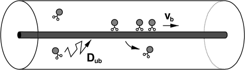
FIG. 1.: Motor particles which can bind and unbind to a filament (dark rod) within a cylindrical tube. Single motors which are bound to the filament (and are not sterically hindered by other motors) move with velocity $v_{\rm b}$ to the right. Unbound motors diffuse with diffusion coefficient $D_{\rm ub}$ in the surrounding liquid.

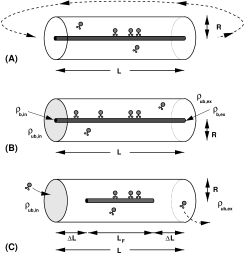
FIG. 2.: Different types of boundary conditions: (A) Periodic boundary conditions which is similar to a closed torus geometry; (B) Open tube with boundaries satisfying radial equilibrium: the bound and unbound motor densities are fixed at the two boundaries and satisfy radial detailed balance at each boundary; and (C) Open tube with diffusive injection and extraction of motors. In all cases, the tube has total length $L$; in cases (A) and (B), the filament has the same length as the tube; in case (C), the filament has length $L_{\rm F}<L$ and there are two boundary compartments of linear size $\Delta L$.

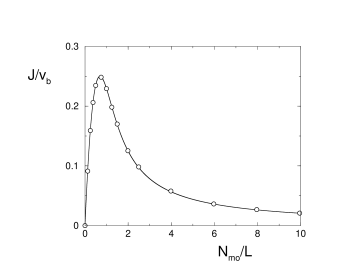
FIG. 3.: Reduced current $J/v_{\rm b}$ through the tube with periodic boundary conditions as a function of the reduced particle number $N_{\rm mo}/L$. The line is calculated from Eq. (8), the Monte Carlo data are obtained for a tube of length $L=200$ and radius $R=25$ corresponding to channel number $N_{\rm ch}=1940$. The random walk probabilities are $\beta=0$, $\gamma=99/100$, $\epsilon=10^{-4}$, $\alpha=1-\gamma-2\epsilon/3$, and $\pi_{\rm ad}=1$.

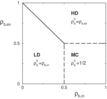
FIG. 4.: Phase diagram for motor traffic in open tubes with boundary condition (B) as a function of the boundary densities $\rho_{\rm b,in}$ and $\rho_{\rm b,ex}$ at the left and right end of the filament, respectively. There are three phases distinguished by the bulk value of the bound density $\rho_{\rm b}^{0}$: a low density phase (LD), a high density phase (HD), and a maximal current phase (MC). This phase diagram is identical to the phase diagram of the 1–dimensional ASEP as explained in the text.

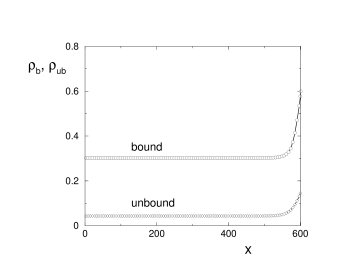
FIG. 5.: Bound and unbound density profiles $\rho_{\rm b}$ and $\rho_{\rm ub}$ as a function of the spatial coordinate $x$ for the low density phase with boundary conditions (B) and boundary densities $\rho_{\rm b,in}=0.3$ and $\rho_{\rm b,ex}=0.6$. The unbound density has been averaged over the tube cross section and multiplied by a scale factor of 10. All data points are averages over six lattice sites in direction parallel to the filament. The tube has length $L=600$ and radius $R=10$. The random walk probabilities are $\beta=\gamma=0$, $\epsilon=10^{-2}$, $\alpha=1-2\epsilon/3$, and $\pi_{\rm ad}=1$.

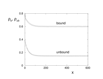
FIG. 6.: Bound and unbound density profiles $\rho_{\rm b}$ and $\rho_{\rm ub}$ as functions of the spatial coordinate $x$ for the high density phase; boundary conditions (B) with $\rho_{\rm b,in}=0.8$ and $\rho_{\rm b,ex}=0.6$. The unbound density has been averaged over the tube cross section and multiplied by a scale factor of 10. The geometry and the random walk probabilities are the same as in Fig. 5.

FIG. 7.: Localization length $\xi$ as a function of the tube radius $R$ for boundary conditions (B) with $\rho_{{\rm b},\rm in}=0.38$ and $\rho_{{\rm b},\rm ex}=0.6$. Circles are simulation data, obtained for a tube with length $L=600$ and with random walk probabilities as in Fig. 5; lines are the corresponding results of mean field calculations (dotted: discrete two-state approximation, dashed: continuous two-state approximation, solid: full diffusion equation, see text). The two crosses and the filled circle at $R=0$ represent the mean field results and the exact result for the 1–dimensional ASEP, respectively.

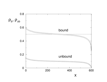
FIG. 8.: Bound and unbound density profiles $\rho_{\rm b}$ and $\rho_{\rm ub}$ as functions of the spatial coordinate $x$ for the maximal current phase; boundary conditions (B) with $\rho_{\rm b,in}=0.6$ and $\rho_{\rm b,ex}=0.1$. The unbound density has been averaged over the tube cross section and multiplied by a scale factor of 10. The parameters are the same as in Fig. 5.

FIG. 9.: Deviation $\eta_{\rm b}$ of the bound density from its constant value far from the boundaries as a function of the spatial coordinate $x$ for the 1–dimensional ASEP (solid line) and for motor traffic in tubes with radius $R=3,5,7$ (dashed lines) and boundary conditions (B) with $\rho_{\rm b,in}=0.8$ and $\rho_{\rm b,ex}=0.5$. The curves for the 1–dimensional ASEP and for the tube radii $R=3,5$ have been multiplied by scale factors 0.1, 0.2, and 0.5, respectively. The thin dotted lines correspond to the decay laws $\sim 1/x$ and $\sim 1/\sqrt{x}$, respectively. The tube length is $L=2000$ and the random walk probabilities as in Fig. 5.

FIG. 10.: Deviation $\eta_{\rm b}$ of the bound density from its constant value far from the boundaries as a function of the spatial coordinate $x$ for a tube with radius $R=3$ and length $L=6000$; boundary conditions (B) with $\rho_{\rm b,in}=0.8$ and $\rho_{\rm b,ex}=0.5$. The thin solid line is obtained from the simulation, the thick dashed line is a fit to Eq. (25) with $D_{sc}\simeq 0.81$ and $x_{sc}\simeq 8.57$. The dotted line indicates the power law $\sim 1/\sqrt{x}$. Note that the simulation data decay faster than $\sim 1/\sqrt{x}$ for $10^{1}\mathrel{\mathchoice{\vbox{\offinterlineskip\halign{\hfil$\displaystyle#$\hfil\cr<\cr\sim\cr}}}{\vbox{\offinterlineskip\halign{\hfil$\textstyle#$\hfil\cr<\cr\sim\cr}}}{\vbox{\offinterlineskip\halign{\hfil$\scriptstyle#$\hfil\cr<\cr\sim\cr}}}{\vbox{\offinterlineskip\halign{\hfil$\scriptscriptstyle#$\hfil\cr<\cr\sim\cr}}}}x\mathrel{\mathchoice{\vbox{\offinterlineskip\halign{\hfil$\displaystyle#$\hfil\cr<\cr\sim\cr}}}{\vbox{\offinterlineskip\halign{\hfil$\textstyle#$\hfil\cr<\cr\sim\cr}}}{\vbox{\offinterlineskip\halign{\hfil$\scriptstyle#$\hfil\cr<\cr\sim\cr}}}{\vbox{\offinterlineskip\halign{\hfil$\scriptscriptstyle#$\hfil\cr<\cr\sim\cr}}}}10^{2}$. The random walk probabilities are the same as in Fig. 5.

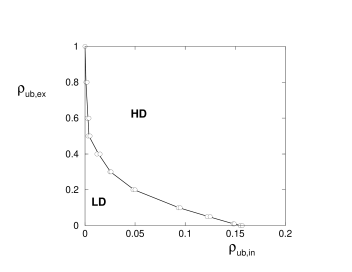
FIG. 11.: Phase diagram for tubes with boundary conditions (C) as a function of the left and right boundary densities $\rho_{\rm ub,in}$ and $\rho_{\rm ub,ex}$ for a set of parameters where no maximal current phase occurs. The tube has length $L=600$ and radius $R=5$, the filament length is $L_{F}=590$ and the distance between the filament ends and the tube ends is $\Delta L=5$. The random walk probabilities are the same as in Fig. 5. Note the different scales of the axes.

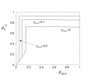
FIG. 12.: Bound density $\rho_{\rm b}^{0}$ as a function of the left boundary density $\rho_{\rm ub,in}$ for boundary conditions (C) and different values of the right boundary density $\rho_{\rm ub,ex}$. The parameters are the same as in Fig. 11. The discontinuity in the functional dependence of $\rho_{\rm b}^{0}$ on $\rho_{\rm ub,in}$ corresponds to the transition from the low to the high density phase, compare Fig. 11.

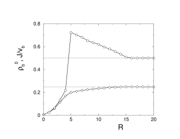
FIG. 13.: Current $J/v_{\rm b}$ (diamonds) and bound density $\rho_{\rm b}^{0}$ (circles) as a function of the tube radius $R$ for boundary conditions (C) with $\rho_{\rm ub,in}=0.2$, $\rho_{\rm ub,ex}=0$. The tube length $L=600$, the filament length $L_{F}=590$, and the distance between the filament ends and the tube ends is $\Delta L=5$. The random walk probabilities are the same as in Fig. 5.

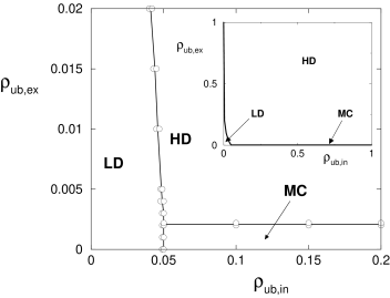
FIG. 14.: Phase diagram for a tube of radius $R=17$ with boundary conditions (C) as a function of the left and right boundary densities $\rho_{\rm ub,in}$ and $\rho_{\rm ub,ex}$. The other parameters are the same as in Fig. 11. In the inset, which shows the complete phase diagram, the maximal current phase can be hardly distinguished from the line $\rho_{\rm ub,ex}=0$.

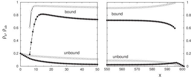
FIG. 15.: Bound and unbound density profiles $\rho_{\rm b}$ and $\rho_{\rm ub}$ as functions of the spatial coordinate $x$ for boundary conditions (C) with $\rho_{\rm ub,in}=0.2$ and $\rho_{\rm ub,ex}=0$. Two different unbinding processes of the motor particles at the ’last’ filament site are compared: (Filled circles) Active unbinding for which the motor makes one final step in the forward direction; and (Open Circles) Thermal unbinding with probability $\epsilon/6$ in the forward direction. The geometric parameters are $L=600$, $L_{F}=590$, $\Delta L=5$, and $R=5$; the random walk probabilities are as in Fig. 5.

REFERENCES

- [1] J. Howard. Mechanics of motor proteins and the cytoskeleton. Sinauer Associates, Sunderland (Mass.), 2001.
- [2] G. Woehlke and M. Schliwa. Walking on two heads: the many talents of kinesin. Nature Reviews Molec. Cell Biol., 1:50–59, 2000.
- [3] R. D. Vale, T. Funatsu, D. W. Pierce, L. Romberg, Y. Harada, and T. Yanagida. Direct observation of single kinesin molecules moving along microtubules. Nature, 380:451–453, 1996.
- [4] K. S. Thorn, J. A. Ubersax, and R. D. Vale. Engineering the processive run length of the kinesin motor. J. Cell Biol., 151:1093–1100, 2000.
- [5] R. Lipowsky, S. Klumpp, and Th. M. Nieuwenhuizen. Random walks of cytoskeletal motors in open and closed compartments. Phys. Rev. Lett., 87:108101.1–4, 2001.
- [6] Th. M. Nieuwenhuizen, S. Klumpp, and R. Lipowsky. Walks of motors in two and three dimensions. Europhys. Lett., 58:468–474, 2002.
- [7] S. Katz, J. L. Lebowitz, and H. Spohn. Nonequilibrium steady states of stochastic lattice gas models of fast ionic conductors. J. Stat. Phys., 34:497–537, 1984.
- [8] A. B. Kolomeisky, G. M. Schütz, E. B. Kolomeisky, and J. P. Straley. Phase diagram of one-dimensional driven lattice gases with open boundaries. J. Phys. A: Math. Gen., 31:6911–6919, 1998.
- [9] C. T. MacDonald, J. H. Gibbs, and A. C. Pipkin. Kinetics of biopolymerization on nucleic acid templates. Biopolymers, 6:1–25, 1968.
- [10] C. T. MacDonald and J. H. Gibbs. Concerning the kinetics of polypeptide synthesis on polyribosomes. Biopolymers, 7:707–725, 1969.
- [11] H. M. Dintzis. Assembly of the peptide chains of hemoglobin. Proc. Natl. Acad. Sci. USA, 47:247–261, 1961.
- [12] M. A. Naughton and H. M. Dintzis. Sequential biosynthesis of the peptide chains of hemoglobin. Proc. Natl. Acad. Sci. USA, 48:1822–1830, 1962.
- [13] R. M. Winslow and V. M. Ingram. Peptide chain synthesis of human hemoglobin A and A2*. J. Biol. Chem., 241:1144–1149, 1966.
- [14] F. Spitzer. Interaction of Markov processes. Adv. Math., 5:246–290, 1970.
- [15] J. Krug. Boundary-induced phase transitions in driven diffusive systems. Phys. Rev. Lett., 67:1882–1885, 1991.
- [16] G. Schütz and E. Domany. Phase transitions in an exactly soluble one-dimensional exclusion process. J. Stat. Phys., 72:277–296, 1993.
- [17] B. Derrida, M. R. Evans, V. Hakim, and V. Pasquier. Exact solution of a 1D asymmetric exclusion model using a matrix formulation. J. Phys. A: Math. Gen., 26:1493–1517, 1993.
- [18] T. M. Liggett. Stochastic Interacting Systems: Contact, Voter and Exclusion Processes. Springer, Berlin, 1999.
- [19] V. Popkov, L. Santen, A. Schadschneider, and G. M. Schütz. Empirical evidence for a boundary-induced nonequilibrium phase transition. J. Phys. A: Math. Gen., 34:L45–L52, 2001.
- [20] L. S. B. Goldstein and Z. Yang. Microtubule-based transport systems in neurons: The roles of kinesins and dyneins. Annu. Rev. Neurosci., 23:39–71, 2000.
- [21] A. B. Dahlström, K. K. Pfister, and S. T. Brady. The axonal transport motor ’kinesin’ is bound to anterogradely transported organelles: quantitative cytofluorimetric studies of fast axonal transport in the rat. Acta Physiol. Scand., 141:469–476, 1991.
- [22] H. van Beijeren, R. Kutner, and H. Spohn. Excess noise for driven diffusive systems. Phys. Rev. Lett., 54:2026–2029, 1985.
- [23] K. H. Janssen and K. Oerding. Renormalized field theory and particle density profile in driven diffusive systems with open boundaries. Phys. Rev. E, 53:4544-4554, 1996.
- [24] J. S. Hager, J. Krug, V. Popkov, and G. M. Schütz. Minimal current phase and universal boundary layers in driven diffusive systems. Phys. Rev. E, 63:056110/1-056110/12, 2001.
- [25] T. Surrey, F. Nédélec, S. Leibler, and E. Karsenti. Physical properties determining self-organization of motors and microtubules. Science, 292:1167–1171, 2001.
- [26] S. Klumpp and R. Lipowsky. To be published.
- [27] G. M. Schütz. Exactly solvable models for many-body systems far from equilibrium. In C. Domb and J. L. Lebowitz, editors, Phase Transitions and Critical Phenomena, volume 19, pages 1–251. Academic Press, San Diego, 2001.