Reflectivity of cholesteric liquid crystals with spatially varying pitch

Abstract

Solids with spatially varying photonic structure offer gaps to light of a wider range of frequencies than do simple photonic systems. We solve numerically the field distribution in a cholesteric with a linearly varying inverse pitch (helical wavevector) using equations we derive for the general case. The simple idea that the position where the Bragg condition is locally satisfied is where reflection takes place is only true in part. Here, reflection is due to a region where the waves are forced to become evanescent, and the rate of variation of structure determines over which distance the waves decay and therefore how complete reflection is. The approximate local Bragg-de Vries schemes are shown to break down in detail at the edges of the gap, and an analytical estimate is given for the transmission coefficient.

1 Introduction

Photonic band structures can be made to vary spatially by varying the lattice repeat distance as one penetrates the sample. An example where this technique has been used with great success is that of cholesterics. In such liquid crystals the director (the direction of high refractive index) rotates on moving perpendicularly to itself to give a helical structure, see the sketch fig. 1. These structures are known devries51 to have a single photonic stop gap for normal incidence of circularly polarized light of the same handedness as the helical cholesteric and no gap for light of the opposite handedness.

We study here variable pitch cholesterics (VPCs). The motivation for spatially varying structures is to have reflection over a broader range of frequencies than simply that provided by the gap of a uniform system. This has been usefully employed in wide band reflectors and circular polarizers for display purposes. The idea employed to interpret such effects is that light of a given frequency penetrates until the repeat distance of the solid is locally that of the wavelength of this light in the solid. At this point a Bragg-de Vries condition is satisfied and reflection occurs. Our purpose is to explore whether such an approach has any utility and what limitations arise, for instance unwittingly allowing unwanted transmission under some circumstances. The counter argument to this simple argument would be that Bragg effects are coherent – one needs very many such repeats to get sharp and total Bragg interference and in a varying medium this is achieved nowhere. To some extent the answer must be that significant evanescence of the wave must occur between first encountering the gap and leaving it. We explore this numerically and by approximate methods. A rather different theoretical approach has used the Berreman matrix formulation lu-li97 .

Since cholesterics are locally nematic and therefore also fluid, a VPC must be solidified to stabilize the pitch gradient once it has been set up. One method is to photo-induce a concentration gradient in a blend of chiral and achiral photo-crosslinkable mesogens Broer ; Broer_99 . A network (elastomer) is formed which freezes in the structure. Otherwise, thermal diffusion between two cholesteric layers with different pitches can be used to set up a variation in pitch which can then be frozen in by quenching to the glassy state mitov-boudet98 .

2 Governing equations

In conventional cholesteric liquid crystals, the nematic director $\bm{n}$ rotates uniformly in a plane as one advances in a line perpendicular to this plane. We shall adopt the following convention: the nematic director $\bm{n}$ is confined to the $xy$-plane, and the direction in which the director changes is therefore the $z$-axis, see fig. 1. The director of ordinary cholesteric liquid crystals subsequently becomes

$$\bm{n}=\left(\cos\phi(z),\sin\phi(z),0\right)\quad\mbox{with}\quad\phi(z)=\frac{2\pi}{p_{0}}z,$$ (1)

where $p_{0}$ is the pitch length.

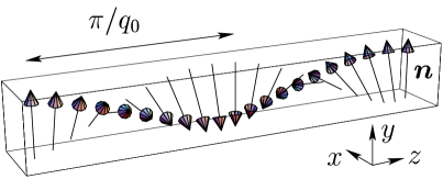
Figure 1: A classical, constant pitch cholesteric structure. The arrows indicate the nematic director prevalent in the $xy$-plane at a certain $z$ coordinate. Note that $\bm{n}$ and $-\bm{n}$ describe the same physical state, namely an orientational order along the direction of $\bm{n}$ (or $-\bm{n}$).

To allow for the most general phase evolution, we look at the governing equation for electromagnetic waves in a cholesteric liquid crystal whose pitch does not need to be a constant. In other words, we do not assume the specific form $\phi=(2\pi/p_{0})z$ in eq. (1), but leave the phase in the most general form $\phi(z)$. On the other hand, we restrict ourselves to electromagnetic waves which propagate along the $z$-axis only, i.e. perpendicular to the director $\bm{n}$. Therefore the electric and magnetic fields of the wave only have $x$ and $y$ components jackson75 .

The anisotropy of the liquid crystalline phase described by the director $\bm{n}$ implies that locally the dielectric tensor respects the uniaxial symmetry of the liquid crystalline phase. It therefore assumes the following form:

$$\underline{\underline{{\bm{\epsilon}}}}=\epsilon_{1}\underline{\underline{{\bm{\delta}}}}+\left(\epsilon_{2}-\epsilon_{1}\right)\bm{n}\bm{n}^{\sf T},$$ (2)

where $\underline{\underline{{\bm{\delta}}}}$ is the $3\times 3$ unit matrix and where $\epsilon_{2}$ and $\epsilon_{1}$ are the dielectric constants parallel and perpendicular to the director $\bm{n}$ respectively. Since $\bm{n}$ rotates in the $xy$-plane along the $z$-axis eq. (1), the dielectric tensor $\underline{\underline{{\bm{\epsilon}}}}$ eq. (2) depends too on the $z$-coordinate.

In the present case, the electromagnetic wave equation (assuming a unit magnetic permeability $\mu=1$), reads jackson75 :

$$\frac{1}{c^{2}}\frac{\partial^{2}\bm{D_{t}}}{\partial t^{2}}=\frac{\partial^{2}\bm{E_{t}}}{\partial z^{2}},$$ (3)

with the dielectric displacement field $\bm{D_{t}}=\underline{\underline{{\bm{\epsilon}}}}\bm{E_{t}}$.

Introducing the time dependence $\bm{E_{t}}(z)=e^{i\omega t}\bm{E}(z)$ (and similarly for $\bm{D}$), all time derivatives become a mere multiplication by $i\omega$, and we obtain:

$$-k_{0}^{2}\bm{D}=\frac{\partial^{2}\bm{E}}{\partial z^{2}}\ \mbox{with}\ k_{0}=\frac{\omega}{c}.$$ (4)

Note that the tensor $\underline{\underline{{\bm{\epsilon}}}}$ is in general not diagonal in the fixed laboratory frame $(xyz)$ (cf. eqs. (1) and (2)), however due to its symmetry given by eq. (2), the dielectric tensor is diagonal in the frame defined by the rotating director $\bm{n}(z)$. In this frame, which we denote by a tilde and $(\xi,\eta)$ coordinates, the electric displacement field is simply given by:

$$\tilde{D}_{\xi}=\epsilon_{1}\tilde{E}_{\xi}\ \mbox{and}\ \tilde{D}_{\eta}=\epsilon_{2}\tilde{E}_{\eta}.$$ (5)

We take $\eta$ to be the direction along $\bm{n}$ and hence typically $\epsilon_{2}>\epsilon_{1}$.

The coordinate transform into the rotating frame (attached to the director $\bm{n}$), reads as follows:

$$\tilde{\bm{E}}=\underline{\underline{{\bm{R}}}}(z)\bm{E}\ \mbox{with}\ \underline{\underline{{\bm{R}}}}(z)=\begin{pmatrix}\cos\phi(z)&\sin\phi(z)\\ -\sin\phi(z)&\cos\phi(z)\\ \end{pmatrix}.$$ (6)

In this new frame, eq. (4) transforms into

$$k_{0}^{2}\,\underline{\underline{{\bm{\epsilon}}}}\,\tilde{\bm{E}}=\begin{pmatrix}-\partial^{2}_{z}+\phi^{\prime}&2\phi^{\prime}\partial_{z}+\phi^{\prime\prime}\\ -(2\phi^{\prime}\partial_{z}+\phi^{\prime\prime})&-\partial^{2}_{z}+\phi^{\prime}\\ \end{pmatrix}\tilde{\bm{E}},$$ (7)

where $\partial_{z}=\partial/\partial z$ and $\phi^{\prime}=\partial\phi/\partial z$, and $\underline{\underline{{\bm{\epsilon}}}}$ is now the diagonal $2\times 2$ dielectric tensor $\begin{pmatrix}\epsilon_{1}&0\\ 0&\epsilon_{2}\\ \end{pmatrix}$ in the $(\xi,\eta)$ frame. Dropping the tilde, here and henceforth, eq. (7) reads:

$$k_{0}^{2}\,\epsilon_{1}\,E_{\xi} = -E_{\xi}^{\prime\prime}+E_{\xi}\phi^{\prime 2}+2E_{\eta}^{\prime}\phi^{\prime}+E_{\eta}\phi^{\prime\prime}$$

$$k_{0}^{2}\,\epsilon_{2}\,E_{\eta} = -E_{\eta}^{\prime\prime}+E_{\eta}\phi^{\prime 2}-2E_{\xi}^{\prime}\phi^{\prime}-E_{\xi}\phi^{\prime\prime}.$$ (8)

3 Cholesterics with constant pitch

Ordinary cholesteric liquid crystals are characterised by a constant pitch $p_{0}$. Hence the director $\bm{n}$ performs a steady rotation as one travels in $z$-direction. The physical system is periodic in $\frac{p_{0}}{2}$, although eq. (1) is only periodic in $p_{0}$, reflecting the fact that both $\bm{n}$ and $-\bm{n}$ describe the axis of anisotropy of a uniaxial system equally well, see eq. (2).

For constant pitch, the phase $\phi(z)$ is given by $\phi=q_{0}z$ with $q_{0}=\frac{2\pi}{p_{0}}={\rm const.}$ and hence $\phi^{\prime}=q_{0}$ and $\phi^{\prime\prime}=0$ – the classical problem of de Vries. The wave equation (8) is exactly solvable devries51 in the $(\xi,\eta)$ frame using the solution:

$$\bm{E}=\begin{pmatrix}A\\ iB\\ \end{pmatrix}e^{ikz}\;.$$ (9)

We obtain two linear homogeneous equations for the coefficients $A$ and $B$. There can only be a non-trivial solution if the determinant of the corresponding matrix equals zero:

$$k^{4}-k^{2}(k_{0}^{2}[\epsilon_{1}+\epsilon_{2}]+2q_{0}^{2})+(\epsilon_{1}k_{0}^{2}-q_{0}^{2})(\epsilon_{2}k_{0}^{2}-q_{0}^{2})=0\;.$$ (10)

This quadratic equation in $k^{2}$ establishes a relationship between the temporal frequency $\omega=k_{0}c$ and the corresponding wave vector $k$. In the reduced zone scheme, the relationship $k_{0}$ as a function of $k$ is shown in fig. 2(a).

Figure 2: (a) Reduced temporal frequency $k_{0}=\omega/c$ vs. wave vector $k$: in a cholesteric liquid crystal with constant pitch $p_{0}$, there are two pairs of solutions. One of them exhibits a single stop gap for normal incidence at frequencies $k_{0}=\omega/c$ between $[q_{0}/\sqrt{\epsilon_{2}},q_{0}/\sqrt{\epsilon_{1}}]$ (solid line) with $q_{0}$ being the cholesteric’s wave vector $2\pi/p_{0}$. The other is gapless (dashed line). The plot can be extended to negative values of $k$ by reflection in the $k_{0}$-axis. In this example, we arbitrarily chose $\epsilon_{1}=2.25$, $\epsilon_{2}=3.24$ (the dielectric constants perpendicular and parallel to the local director) and $q_{0}=1$. (b) The corresponding ratio of the fields along and perpendicular to the rotating director as a function of frequency $k_{0}=\omega/c$. The dotted line of the inset shows how the ratio $A/B$ becomes imaginary in the gap and that the variation of $A/B$ is strong near the edges of the gap.

The ratio $A/B=E_{\xi}/E_{\eta}$ of the field components also varies as $k(k_{0})$ is varied:

$$\frac{A}{B}(k_{0})=\frac{2kq_{0}}{k^{2}+q_{0}^{2}-\epsilon_{2}k_{0}^{2}}\;,$$ (11)

where $k$ and $k_{0}$ are related by eq. (10), see fig. 2(b). The choice of the dielectric constants $\epsilon_{1}$ and $\epsilon_{2}$ in this illustration corresponds to refractive indices perpendicular and parallel to $\bm{n}$ of $n_{1}=1.5$ and $n_{2}=1.8$.

Equation (10) allows two pairs of solutions: for each fixed frequency $k_{0}=\frac{\omega}{c}$, there are two solutions whose wave vector $k$ have the same magnitude, but opposite sign, reflecting the fact that there are waves travelling in the two opposite directions along the $z$-axis. Apart from this trivial pairing, there are two genuinely different solutions to eq. (10). One of them exhibits a band gap in the frequency range $\omega/c\in[q_{0}/\sqrt{\epsilon_{2}},q_{0}/\sqrt{\epsilon_{1}}]$. Note that due to the periodicity in the cholesteric structure, the graphs in fig. 2(a) were shifted by 1 along the $k$-axis to yield the reduced zone representation.

The non-trivial pair of solutions, the de Vries eigenstates, are in general of elliptical polarization, the principal directions of which rotate with $\bm{n}$. At the two band edges at $k_{0}=q_{0}/\sqrt{\epsilon_{2}}$ and $q_{0}/\sqrt{\epsilon_{1}}$, the states are plane polarized with the plane of polarization rotating with $\bm{n}$.

Light with the same handedness as the cholesteric has states $(E_{\xi},0)$ and $(0,E_{\eta})$ at the band edges, corresponding to $\bm{E}$ respectively along $\bm{n}$ or perpendicular to $\bm{n}$. The ratio $A/B$ is then $\infty$ or 0 respectively. The former is along a polarizable direction and hence produces a lower energy that the latter even though the spatial variation $k$ is the same — a gap has been produced. Light rotating with the opposite handedness does not couple coherently to the cholesteric and retains a gapless dispersion relation, the dashed line in fig. 2. The de Vries problem, in this photonic band structural language of fig. 2, can be extended to non-uniform but periodical director rotation bermel-warner02 .

4 Cholesterics with varying pitch

In varying pitch cholesterics (VPCs) the nematic director $\bm{n}$ rotates non-uniformly along the $z$-axis, i.e., the phase $\phi(z)$ of eq. (1) does not have the simple form $\phi(z)=q_{0}z=2\pi z/p_{0}$ with $q_{0}={\rm const}$, but assumes a more general form. It has been reported that the local pitch can vary exponentially with $z$ lu-li97 , i.e., we can write $q=q_{0}\exp(-\kappa z)$. Other careful, scanning electron microscopy investigations Broer ; Broer_99 ; mitov-boudet98 , showed the pitch to be linear over a range of $z$-values. Here, we assume the simplest possible inverse pitch variation, namely a linear dependency on $z$, leading to a quadratic dependence of the phase $z$:

$$q=q_{0}+\gamma q_{0}^{2}z\ \Longrightarrow\ \phi(z)=\left(q_{0}+\textstyle{\frac{1}{2}}\gamma q_{0}^{2}z\right)z\;.$$ (12)

4.1 Local de Vries approximation

A simple framework for considering a wide band circular polarizer, filter or reflector now presents itself Broer ; Broer_99 ; mitov-boudet98 . As light of a given frequency enters and accordingly has a given wavelength in the medium, then since $q(z)$ changes, there will be a depth at which a Bragg-like condition will be satisfied, and at this depth the wave will be totally reflected. This is where the wavelength in the medium matches the local periodicity $2\pi/q(z)$. We examine how much credence to put in this description. For Bragg reflection to occur, one requires a semi infinite medium, at least a thickness of sample corresponding to very many wavelengths. In the variable pitch cholesteric, the Bragg condition is met strictly only at a point and a Bragg mechanism fails. Indeed, instead of a total reflection, there may be circumstances where it is only partial, as we find below.

One can take an analogous approach of applying de Vries theory locally to argue for reflection of light of a given wavelength at the particular point in the VPC where for light at this frequency a de Vries gap is encountered.

In the constant pitch case, one can determine an eigen wave vector $k$ given a frequency $\omega$ (or equivalently $k_{0}$), see fig. 2. The pitch wave vector $q_{0}$ played the role of a parameter in the function $k=k(\omega)$. Let us now change perspective and consider the frequency $\omega$ or $k_{0}=\frac{\omega}{c}$ as a parameter, but allow the inverse pitch length $q$ to change according to eq. (12). In the following, we choose $k_{0}=\frac{\omega}{c}=2$, $\epsilon_{1}=2.25$, $\epsilon_{2}=3.24$, $q_{0}=1$, and $\gamma=0.05$.

By this reasoning, we are able to determine a wave vector $k$ satisfying the de Vries condition eq. (10) given a particular cholesteric inverse pitch length $q$, which in turn depends on the $z$-coordinate by means of eq. (12). Hence, we can plot an hypothetical wave vector $k$ against the local position $z$, fig. 3. Note that for a given frequency $k_{0}$, there are again four solutions derived from eq. (10). Figure 3 only shows two branches, one of them becoming imaginary between $z_{1}$ and $z_{2}$, with $z_{i}=\frac{1}{q_{0}^{2}\gamma}\left(\sqrt{\epsilon_{i}}k_{0}-q_{0}\right)$.

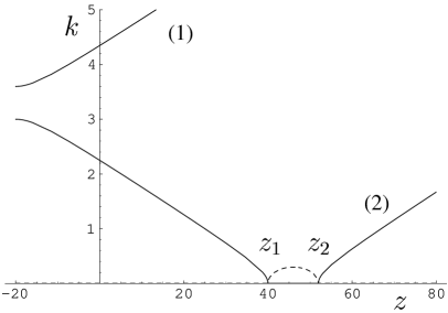
Figure 3: Two of the four branches of the local wave vector $k$ vs. $z$-coordinate: assuming a fixed frequency $k_{0}$, eq. (10) links the wave vector $k$ and the inverse pitch length $q_{0}$. Previously, $q_{0}$ was taken to be a constant, but eq. (12) introduces a dependence on the $z$-coordinate. Thereby, the relation between the wave vector $k$ and the local inverse pitch length $q$ becomes a function of $z$. For this plot, we have chosen $\epsilon_{1}=2.25$, $\epsilon_{2}=3.24$, $k_{0}=2$, $q_{0}=1$, and $\gamma=0.05$ ($q_{0}^{2}\gamma$ being the spatial rate of change of cholesteric wavevector) . With this choice of parameters, the frequency $k_{0}$ lies below the forbidden frequency range at $z=0$. The forbidden zone of branch (2) extends over the region $z\in[z_{1},z_{2}]=[40,52]$.

The second pair of branches can be constructed trivially by introducing minus signs: $k\mapsto-k$. In the region $[z_{1},z_{2}]$ where the frequency $k_{0}$ falls into the band gap for two of the four branches, the corresponding wave vector $k$ becomes imaginary, indicating an evanescent behaviour of the wave. We expect there a decaying and increasing solution (see eq. (9) for imaginary $k$).

One can now return to the question of reflection, or equivalently transmission. The band gap starts at $z_{1}$ and extends to $z_{2}$. Transmission depends on how close $z_{2}$ is to $z_{1}$ and how rapid the exponential decay in this gap is.

4.2 Numerical investigation

The above tentative interpretation of the solution being locally de Vries-like is qualitatively confirmed by looking at a full numerical solution in fig. 4. Here, we have chosen the initial conditions at $z=0$ such that we obtain a decaying solution in the forbidden zone as opposed to an increasing solution, which one obtains for different initial conditions.

Figure 4: Numerical solution of eq. (8) with $\phi(z)=(q_{0}+\frac{1}{2}\gamma q_{0}^{2}z)z$: the initial conditions at $z=0$ are chosen such that the solution decays over the evanescent range $z\in[z_{1},z_{2}]=[40,52]$. The numerical parameters are the same as in fig. 3, and the initial conditions as follows: $E_{\xi}(0)=-0.036$, $E_{\eta}(0)=-0.58$, $E_{\xi}^{\prime}(0)=2.0$, and $E_{\eta}^{\prime}(0)=-0.067$ (the fields and their gradients in the rotating frame $(\xi,\eta)$ at $z=0$).

From the simultaneous field equations (8) for $E_{\xi}$ and $E_{\eta}$, it is clear that one could divide through by a constant, say $E_{\eta}(z=0)$. The required 4 boundary conditions then reduce to 3 choices, the 4th being thus set to $E_{\eta}=1$ at $z=0$, reflecting the arbitrariness of the overall scale in the problem.

Several features of this solution are important for what follows. The amplitudes on either side of the gap region differ considerably. The small amplitude to the right of the gap after partial transmission gives a small Poynting flux, $\bm{E}\wedge\bm{H}$, of energy in the positive $z$ direction. Although the amplitudes on the left are much larger, they correspond to the sum of an incident and reflected wave resulting in a correspondingly small Poynting vector. The ratio $A/B$ of the field amplitudes is approximately constant away from the band edges at $z_{1}$ and $z_{2}$. In the de Vries, constant pitch solution this ratio is respectively $\infty$ and $0$ at these points, extreme values that are not achieved in this case of partial barrier penetration. The ratio also becomes very large at $z=-20$ which for our value $0.05$ of $\gamma$ is the point where there is no rotation of the director at all, that is where $q(z)\rightarrow 0$. Locally the medium is achiral and there is no need for the two-component, de Vries-like solution.

One can now qualitatively analyze reflection and transmission. With rising $q$ vector on penetrating the VPC, one must eventually reach what would be the lower band edge in a uniform de Vries system. However, the gap translates into a spatial region of decaying gap states, and ultimate transmission is determined by how wide this region is. In particular does significant decay of the wave function occur before the propagating region of $z>z_{2}$ is attained? If not, then transmission is higher and reflection lower. Decay depends therefore in part on the gap’s spatial extent

$$z_{2}-z_{1}=\frac{k_{0}}{q_{0}^{2}\gamma}(\sqrt{\epsilon_{2}}-\sqrt{\epsilon_{1}})$$ (13)

over which decay occurs. Clearly, if the spatial variation is weaker, i.e. $\gamma$ small, then the gap is spatially more extended and decay has a greater length over which to take place (see also the discussion of the transmission coefficient leading up to eq. (19)).

4.3 Approximate solutions

For constant (inverse) pitch, the solution eq. (9) was a plane wave. In the case of a cholesteric with a $z$-dependent (inverse) pitch, we choose a more general trial function, namely a WKB-like (Wentzel, Kramers and Brillouin) ansatz, assuming for simplicity that the two field components $E_{\xi}$ and $E_{\eta}$ share the same phase $S(z)$:

$$\begin{pmatrix}E_{\xi}\\ E_{\eta}\\ \end{pmatrix}=\begin{pmatrix}A\\ iB\\ \end{pmatrix}e^{iS(z)}.$$ (14)

Inserting eq. (14) into the wave equation (8) yields two linear equations for $A$ and $B$, which have a non-trivial solution only if the corresponding determinant is zero. Therefore, the analogous equation to eq. (10) is:

$$+S^{\prime\prime}\gamma^{2}q_{0}^{2}\left(i(\epsilon_{1}+\epsilon_{2})k_{0}^{2}-2iq_{0}^{2}w^{2}-q_{0}^{2}S^{\prime\prime}\right)$$

$$+S^{\prime 4}q_{0}^{4}\gamma^{4}+S^{\prime}4iq_{0}^{4}w\gamma^{2}$$ (15)

$$-S^{\prime 2}\gamma^{2}q_{0}^{2}\left((\epsilon_{1}+\epsilon_{2})k_{0}^{2}+2q_{0}^{2}w^{2}+2iq_{0}^{2}\gamma^{2}S^{\prime\prime}\right)$$

$$\epsilon_{1}\epsilon_{2}k_{0}^{4}-(\epsilon_{1}+\epsilon_{2})k_{0}^{2}q_{0}^{2}w^{2}+q_{0}^{4}w^{4}+q_{0}^{4}\gamma^{2} = 0$$

where we have used a rescaled variable $w=1+q_{0}\gamma z$. Also note that the prime denotes the differentiation with respect to the new variable $w$: $S^{\prime}\equiv\partial S(w)/\partial w$.

This equation is not just an algebraic equation like eq. (10), but rather a non-linear second order differential equation for $S$. An approximation is buried in this procedure. The components $A$ and $B$ were taken as constants, any variation with $z$ they might have in common being taken up as logarithmic terms in the general phase $S(z)$ (including any usual pre-exponential terms like $(S^{\prime})^{-1/4}$ that one would find in conventional WKB). However, we know from eq. (11) and fig. 2(b) that the ratio $A/B$ in the uniform case depends on $k$ which is now varying with respect to $q(z)$ since the pitch is spatially varying. Hence even in a local de Vries picture, $A/B$ must be a function of $z$ through $q(z)$. This variation has been ignored on inserting (14) into eq. (8). The full numerical solution, fig. 4, indeed shows the ratio $A/B$ to vary spatially. From fig. 2(b), one can see that the de Vries value is $\infty$ at the lower edge and $0$ at the upper. However, the variation $A/B$ goes to zero as $\gamma\rightarrow 0$, as expected, and can be estimated for small $\gamma$ to be proportional to $\gamma k_{0}$, implying a small variation of $A/B$ for small $\gamma$.

Furthermore, the form (14) is expected to be valid in the regions where the variation $A/B$ is small. By looking at fig. 2 with the axes interchanged, one recognizes that the variation of $A/B$ is strong near the gap edges, but weak otherwise.

Ignoring this potential shortcoming in the ansatz (14), and neglecting terms involving $S^{\prime\prime}(w)$, the determinental consistency equation (15) for $A$ and $B$ reduces to a 4th order algebraic equation for $S^{\prime}(w)$. This equation can be solved analytically, giving a very long and complicated expression $S_{1}^{\prime}$ for this approximation to $S^{\prime}(w)$.

In fig. 5 we compare this solution $S_{1}^{\prime}$ to a further simplified approach: after switching back to the old $z$ variable, we take $\gamma\rightarrow 0$ to obtain $S_{2}^{\prime}$; this corresponds exactly to the de Vries wavevector function derived from eq. (10) and used in fig. 3: $S_{2}^{\prime}$ stands for the local wave vector $k(z)$ of a plane wave with frequency $\omega=k_{0}c$ in a cholesteric with a inverse pitch $q(z)$, which we consider as locally constant – thus taking $\gamma=0$ here means that we ignore derivatives of the phase $\phi$, in other words an adiabatic approximation:

$$S_{2}^{\prime} = \pm\Big{(}\textstyle{\frac{1}{2}}k_{0}^{2}(\epsilon_{1}+\epsilon_{2})+q^{2}$$

$$\ \pm\textstyle{\frac{1}{2}}k_{0}\sqrt{(\epsilon_{1}-\epsilon_{2})^{2}k_{0}^{2}+8q^{2}(\epsilon_{1}+\epsilon_{2})}\Big{)}^{1/2},$$

where $q=q(z)$ again is given by eq. (12).

Figure 5: Comparison of the two approximations made: we plot the relative error $(|S_{1}^{\prime}-S_{2}^{\prime}|)/|S_{1}^{\prime}|$ between the two approximations $S_{1}^{\prime}$ and $S_{2}^{\prime}$ over the $z$-range. The two lines correspond to the two solutions, see the two branches in fig. 3. In the case of the branch with the forbidden zone (continuous line), the approximation (4.3) for obtaining $S_{2}$ is valid a long distance away from the points $z_{1}$ and $z_{2}$, but breaks down in their vicinity.

We note that, for the branch with the forbidden zone, the approximation which takes us from $S_{1}^{\prime}$ to $S_{2}^{\prime}$ is valid far away from the points $z_{1}$ and $z_{2}$, where the phase variation is zero on the transition from being real to becoming imaginary or vice versa. However, close to these points, approximating $S_{1}^{\prime}$ with $S_{2}^{\prime}$ clearly breaks down, as fig. 5 shows. In any event at the band edges where $S^{\prime}(z)\rightarrow 0$ the WKB-like approach breaks down for the usual reasons.

4.4 Comparison of approximate schemes with numerical solutions

So far, we have only compared the validity of two consecutive approximations $S_{1}^{\prime}$ and $S_{2}^{\prime}$ with each other. However, the true test is to compare the approximation to the full numerical solution.

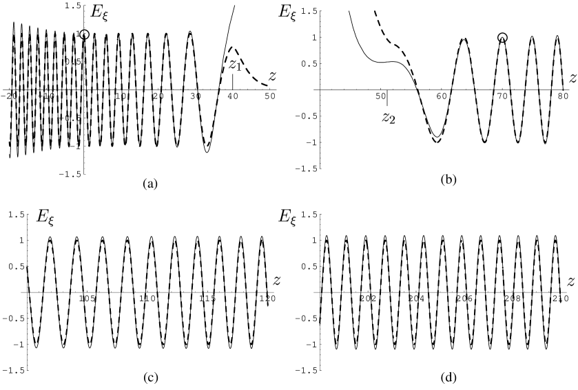
Figure 6: Comparison of the full numerical solution (continuous thin line) and the approximate solution (overlaid dashed line): the approximate solution is based on an numerical integration of the local de Vries expression (4.3) and eq. (14). In fig. (a), the numerical solution is forced to have the same initial conditions at the point $z_{0}=0$, whereas in figs. (b)–(d) $z_{0}=70$ (circled). Plots (c) and (d) demonstrate the stability of the approximate solution for values of positions $z$ distant from $z_{0}$. Note that the $z$-range is different in each of the diagrams (b)–(d) indicating faster oscillations of the field $(E_{\xi},E_{\eta})$ for large $z$ in the same way as $q(z)$ increases according to eq. (12).

Figure 6 compares the numerical solution with the approximate solution obtained by using $S_{2}^{\prime}$. For this purpose, we choose the approximate solution $S_{2}^{\prime}$ corresponding to the branch (2) in fig. 3, integrate it numerically and obtain the resulting wave by eq. (14). The numerical solution is obtained by first evaluating eq. (14) at an anchor point $z_{0}$ giving the four necessary initial conditions: the two field components $E_{\xi}$ and $E_{\eta}$, and their gradients $E_{\xi}^{\prime}$ and $E_{\eta}^{\prime}$. In fig. 6 (a), we chose $z_{0}=0$, and in figs. 6 (b)–(d) $z_{0}=70$. We observe that the agreement between the two solutions breaks down on approaching $z_{1}$ and $z_{2}$. This has a plausible explanation: we have seen in fig. 5 that the approximation $S_{2}^{\prime}$ breaks down near the points $z_{1}$ and $z_{2}$ as in WKB. We therefore expect the corresponding solution of the wave equation that is generated from $S_{2}^{\prime}$ to fail dramatically at the same point.

The discrepancy at $z_{1}$ and $z_{2}$ between the approximate and numerical solution can also be explained from another viewpoint: between $z_{1}$ and $z_{2}$, we ideally expect two fundamental solutions, the one increasing and the other decreasing in an exponential-like fashion. As the procedure described in the last paragraph introduces small errors in the initial conditions at $z_{0}$, the numerically computed solution does carry components of the two fundamental solutions. As $z$ enters the region between $z_{1}$ and $z_{2}$, one solution decays rapidly, but the other (initially only marginally present) increases quickly, becoming the dominant contribution in the region $[z_{1},z_{2}]$. Away from the gap the agreement is very good – over large distances above the gap (indicating great stability) and even backwards to the point $z=-20$ where locally the pitch is infinite.

4.5 Transmission coefficient

One can estimate the dependence of the transmission coefficient on the principal variables $q_{0}$, $\gamma$, $k_{0}$, $\epsilon_{1}$ and $\epsilon_{2}$.

Our system is analogous to the simple quantum mechanical barrier problem for a free particle (see for example davydov76 ; here we have a vector field $\bm{E}$ with two components rather than one): outside a region $[0,l]$, propagation is described by the Schrödinger equation of a free particle with an oscillating wave function and allowing for an incoming and an outgoing wave.

However, in the region $[0,l]$, the particle moves across a potential $V$. If the potential $V$ is constant and greater than the particle’s energy $E$, the solutions to the wave equation are either exponentially decaying or increasing. The reflection or transmission coefficients can easily be calculated exactly. For a general potential barrier $V(z)$, the transmission coefficient can be estimated davydov76 :

$$T\approx\exp\left(-2\frac{1}{\hbar}\int_{0}^{l}dz\sqrt{2m(V(z)-E)}\right).$$

We estimate the transmission coefficient $T$ as the square of the ratio of the fields $E_{\xi}$ or $E_{\eta}$ at $z_{1}$ and $z_{2}$:

$$T\approx\left|\frac{E_{\eta}(z_{2})}{E_{\eta}(z_{1})}\right|^{2}\approx\left|\frac{E_{\xi}(z_{2})}{E_{\xi}(z_{2})}\right|^{2}\approx\left|\frac{e^{iS(z_{2})}}{e^{iS(z_{1})}}\right|^{2}$$

where the latter form arises from our assumption (14). The barrier form of $T$ now yields

$$T = \Big{|}\exp\big{(}2i\big{[}S(z_{2})-S(z_{1})\big{]}\big{)}\Big{|}$$ (17)

$$\approx\exp\left(2i\int_{z_{1}}^{z_{2}}dz\ S_{2}^{\prime}(z)\right),$$

where we have implicitly assumed that the integral of $S_{2}^{\prime}(z)$ over $z$ between $z_{1}$ and $z_{2}$ is purely imaginary, yielding a real number in the final exponential of eq. (17). In the forbidden zone $[z_{1},z_{2}]$, there are two solutions for $S^{\prime}_{2}$ (see. eq. (4.3)); both are purely imaginary, but of opposite signs. Therefore, we have to choose the correct one to be inserted into eq. (17), corresponding to the decaying wave.

The function $S_{2}^{\prime}(z)$ in (4.3) has divergent slopes at the boundary points $z_{2}$ and $z_{1}$ and assumes a maximum in between with

$$S^{\prime}_{2\,{\rm max}}=\frac{\epsilon_{2}-\epsilon_{1}}{\sqrt{8}\sqrt{\epsilon_{1}+\epsilon_{2}}}k_{0}.$$

Therefore one might approximate $S_{2}^{\prime}(z)$ by an ellipse between the points $z_{1}$ and $z_{2}$ with a maximum value of $S^{\prime}_{2\,{\rm max}}$:

$$S^{\prime}_{2}(z) \approx S^{\prime}_{2\,{\rm app}}(z)$$

$$= \frac{1}{\sqrt{2}}\frac{ik_{0}}{\sqrt{\epsilon_{1}+\epsilon_{2}}}\sqrt{\big{(}q-\sqrt{\epsilon_{1}}k_{0}\big{)}\big{(}\sqrt{\epsilon_{2}}k_{0}-q\big{)}}\;,$$

where $q=q_{0}+q_{0}^{2}\gamma z$. Figure 7 shows the $S^{\prime}_{2}(z)$ and overlaid the approximation $S^{\prime}_{2\,{\rm app}}$ of eq. (4.5). The inset shows the relative error $(S^{\prime}_{2}-S^{\prime}_{2\,{\rm app}})/S^{\prime}_{2}$.

Figure 7: Quality of the approximation (4.5) to model the function $S_{2}^{\prime}$ in the evanescent region between $z_{1}$ and $z_{2}$: the thin curve corresponds to the imaginary part of $S_{2}^{\prime}$, whilst the overlaid dashed curve is the approximation according to eq. (4.5). The inset shows the relative error.

Finally, this expression can be integrated analytically to give an estimate for the integral in eq. (17), which corresponds to the area under the curve in fig. 7. We obtain

$$T \approx \exp\left(-\frac{\pi}{\sqrt{2}\,4}\frac{k_{0}^{2}}{q_{0}^{2}\gamma}\frac{\left(\sqrt{\epsilon_{1}}-\sqrt{\epsilon_{2}}\right)^{2}}{\sqrt{\epsilon_{1}+\epsilon_{2}}}\right)$$ (19)

$$= \exp\left(-\frac{\pi}{\sqrt{2}\,4}\frac{q_{0}^{2}\gamma\left(z_{1}-z_{2}\right)^{2}}{\sqrt{\epsilon_{1}+\epsilon_{2}}}\right)$$

using eq. (13) for the scaling of $z_{1}-z_{2}$.

To arrive at this estimate (19) of $T$, we used the approximation $S^{\prime}_{2}(z)$, which breaks down near the edges of the stop gap at $z_{1}$ and $z_{2}$, as fig. 5 shows. However, as one can see from fig. 7, the dominant behaviour of $T$ is determined by the large imaginary values of $S^{\prime}_{2}$. These occur deep inside the stop gap where the approximations are valid.

Our expectation at eq. (13) has been confirmed: the wider the spatial extent of the stop gap the smaller the penetration and hence the lower the transmission. Small $\gamma$, that is slow spatial variation of the band structure, gives lower transmission (however providing that the sample is thicker than the spatial extent of the gap!). One requires $\gamma\ll(n_{2}-n_{1})^{2}(k_{0}/q_{0})^{2}$ for effective reflection at the effective frequency $k_{0}$.

5 Conclusions

The numerical solution of the field amplitudes for light in a spatially varying cholesteric (a photonic solid) has been presented. Fields decay in the region where, for the relevant frequency of light, a uniform cholesteric would have its stop gap. Transmission is low for sufficiently slow variation of the pitch. Thus the simple idea that each component of a broad spectrum of light is reflected where its Bragg (strictly its de Vries) condition is satisfied, is partially borne out.

Approximate field amplitudes are derived by taking this local de Vries condition literally. They are reasonable approximations far from the gap, but less good at the gap, for reasons we discuss.

Slower spatial variation, $\gamma$ of pitch gives much lower transmission, in fact exponentially lower, varying as $e^{-A/\gamma}$. This leads to better utility as broad band reflectors in devices.

- (1) H. de Vries, Acta Cryst. 4, 219 (1951).
- (2) Z.J. Lu et al., Mol. Cryst. Liq. Cryst. 301, 237 (1997).
- (3) D. J. Broer, J. Lub and G. N. Mol, Nature 378, 467 (1995).
- (4) D. J. Broer, G. N. Mol, JAMM van Haaren and J. Lub, Adv. Mat. 11, 573 (1999).
- (5) M. Mitov, A. Boudet, and P. Sopena, Eur. Phys. J. B 8, 327 (1999).
- (6) J. D. Jackson, Classical electrodynamics (Wiley, New York, 1975).
- (7) P. A. Bermel and M. Warner, Phys. Rev. E 65, 056614 (2002).
- (8) A. S. Davydov, Quantum Mechanics (Pergamon Press, Oxford, 1976).