Dark-in-Bright Solitons in Bose-Einstein Condensates with Attractive Interactions

Abstract

We demonstrate a possibility to generate localized states in effectively one-dimensional Bose-Einstein condensates with a negative scattering length in the form of a dark soliton in the presence of an optical lattice (OL) and/or a parabolic magnetic trap. We connect such structures with twisted localized modes (TLMs) that were previously found in the discrete nonlinear Schrödinger equation. Families of these structures are found as functions of the OL strength, tightness of the magnetic trap, and chemical potential, and their stability regions are identified. Stable bound states of two TLMs are also found. In the case when the TLMs are unstable, their evolution is investigated by means of direct simulations, demonstrating that they transform into large-amplitude fundamental solitons. An analytical approach is also developed, showing that two or several fundamental solitons, with the phase shift $\pi$ between adjacent ones, may form stable bound states, with parameters quite close to those of the TLMs revealed by simulations. TLM structures are found numerically and explained analytically also in the case when the OL is absent, the condensate being confined only by the magnetic trap.

I Introduction

The current experimental and theoretical studies of Bose-Einstein condensates (BECs) [1] have attracted a great deal of interest to nonlinear patterns which can exist in them, including dark [2] and bright [3] solitons. Two-dimensional (2D) excitations in the form of vortices were also realized experimentally [4]. Other nonlinear excitations, such as Faraday waves [5], ring dark solitons and vortex necklaces [6] were predicted to occur in BECs.

The behavior of the condensate crucially depends on the sign of the atomic interactions: dark (bright) solitons can be created in BECs with repulsive (attractive) interactions, resulting from the positive (negative) scattering length. Recent experiments have demonstrated that “tuning” of the effective scattering length, including a possibility to change its sign, can be achieved by means of a Feshbach resonance [7].

In this work we demonstrate that another type of localized nonlinear excitations, which may be regarded as dark solitons embedded in bright ones, can be created in attractive BECs. They may also be considered as bound states of two bright solitons with a phase shift $\pi$ between them. In some respects, we follow the path of very recent results of Ref. [8]. These, in turn, were based on earlier works on the so-called twisted localized modes (TLMs) in discrete systems [9]; that is why we apply the same term, TLM, to these solitons of the combined dark-bright type. TLMs in a discrete system are bright solitons in which the field vanishes, changing its sign, at the central point. An alternative way to view a TLM is as a concatenation of an “up-pulse” (i.e., ${\rm sech}(x-x_{1})$) with a “down pulse” (i.e., $-{\rm sech}(x-x_{2})$), where $x_{1}$ and $x_{2}$ are appropriately separated, to form an up-down, two-pulse configuration. Notice, however, that our work is essentially different from Ref. [8], since we focus on the case of BECs with negative scattering length (such as ⁷Li [10] and ⁸⁵Rb [11]), and demonstrate robustness and stability of TLMs in the latter context. These structures, if regarded as effectively dark solitons in the attractive BEC, are the inverse of recently predicted [12] bright solitons in repulsive BECs with an optical lattice. It is expected that a characteristic longitudinal length of the TLM soliton in physical units will be on the order of the wavelength of light which induces the OL, i.e., $\sim 1$ $\mu$m, and the number of atoms in the soliton may typically be $\sim 10^{3}$ – $10^{4}$.

We consider a quasi-1D (cigar-shaped) BEC with negative scattering length, the corresponding normalized Gross-Pitaevskii (GP) equation being [1, 13, 14]

$$iu_{t}=-u_{xx}-|u|^{2}u+\left[\epsilon x^{2}+V_{0}\cos^{2}\left(2\pi x/\lambda\right)\right]u,$$ (1)

where $u(x,t)$ is the macroscopic wave function, $\epsilon$ measures the strength of the parabolic magnetic trap, and the last term accounts for the OL potential created by interference of two counterpropagating coherent light beams [15, 16, 17, 18, 19, 20]. As we consider only (effectively) 1D configurations, the attractive interactions between the atoms (characterized by the negative scattering length) can not produce collapse in the framework of the present model, hence various solitons have a chance to be stable.

It is obvious that scaling invariance of Eq. (1) makes it possible to fix the optical wavelength, setting $k\equiv 2\pi/\lambda=1$. This essentially means that all the remaining length scales of the problem are measured by comparison to the period of the optical lattice which has been fixed to $\pi$. We follow this convention below. The number of atoms in the condensate, given by

$$N=\int_{-\infty}^{+\infty}|u(x)|^{2}dx,$$ (2)

is a dynamical invariant of Eq. (1).

In the next section we report detailed numerical results for TLM solutions in attractive BECs, as modeled by Eq. (1). In section III, we will support some of the numerical findings by analytical considerations. Section IV concludes the paper.

II Numerical results

A Stationary twisted-localized-mode solutions and their linear stability

We seek stationary solutions to Eq. (1) in the form,

$\displaystyle u(x,t)=\exp(-i\mu t)v(x),$

where $\mu$ is the chemical potential, and a real function $v(x)$ obeys the equation

$$\mu v=-v_{xx}-v^{3}+\left[\epsilon x^{2}+V_{0}\cos^{2}(2\pi x/\lambda)\right]v\text{,}$$ (3)

supplemented with free boundary conditions. We have checked that the boundary conditions do not significantly affect the results. The corresponding boundary-value problem was solved by means of a finite-difference discretization. A second order difference scheme with spacing $\Delta x=0.2$ was used to approximate $v_{xx}$. The resulting set of nonlinear algebraic equations was solved by means of a Newton iteration. More details on finite-difference schemes and Newton type methods can be found in [21]. The solutions of interest were obtained by choosing, as the initial condition for the Newton iterations, the following functional form:

$$v(x)=\sum_{j=1}^{n}(-1)^{j}\eta{\rm sech}\left(\frac{\eta}{\sqrt{2}}(x-\xi_{j})\right),\eta\equiv\sqrt{-\mu}.$$ (4)

The ansatz (4) approximates a superposition of nonlinear-Schrödinger (NLS) solitons. The presence of the OL suggests choosing positions of the solitons’ centers, $\xi_{j}$, as $\xi_{j}=j\pi/2$, with some integer $j$. The sign factor $(-1)^{j}$ implies the phase difference $\pi$ between adjacent solitons. This choice of the phase pattern is suggested by the known result that, in the discrete NLS equation, only such a configuration may be stable, see Ref. [22] and references therein. Similar results for a BEC model with elliptic-function potentials were obtained in Ref. [23]. The number $n$ of solitons in the initial ansatz (4) was taken as $n=2$, in order to find the TLM soliton proper, or $n=3$, with the objective to find a bound state of two TLMs, see below. However, it will become clear below that concatenating more of such “building block” structures (such as the ones with $n=2$ or $n=3$) one can, in principle, construct multi-pulse configurations with a larger number ($n$) of elementary pulses.

Once TLM states were found as solutions to Eq. (3) [starting with the initial approximation (4)], their stability was subsequently analyzed by examining the corresponding linearized problem for small perturbations. To this end, the perturbed solution was taken as

$$u(x,t)=e^{-i\mu t}\left\{v(x)+\delta\left[a(x)e^{-i\omega t}+b(x)e^{i\omega^{\star}t}\right]\right\},$$ (5)

where $\delta$ is an infinitesimal amplitude of the perturbation, $a(x)$ and $b(x)$ are eigenfunctions of a perturbation mode, and $\omega$ is the corresponding eigenfrequency; $\ast$ standing for the complex conjugation. Using the ansatz of Eq. (5) to O$(\delta)$, one obtains the linearization problem as an eigenvalue problem where $\omega$ is the corresponding eigenfrequency, while $(a,b^{\star})^{T}$ (where the $T$ denotes transpose), is the corresponding eigenfunction. Using the same finite difference scheme as the one used for computing $v(x)$, we convert this to a matrix eigenvalue problem and find all the eigenvalues of the corresponding matrix. This is done by standard matrix eigenvalue solvers built into Matlab [24]. $\omega$ can, in general, be complex, i.e., $\omega=\omega_{r}+i\omega_{i}$, where the subscripts denote the real and imaginary part of the eigenfrequency. If eigenfrequencies with non-zero imaginary parts exist, they lead to exponential instabilities, while their absence implies linear stability of the solution under consideration. This is monitored by the spectral plane pictures of the imaginary ($\omega_{i}$) versus the real ($\omega_{r}$) part of the eigenfrequency (see e.g., the bottom right panels of Figs. 1-3 below). The presence of even a single $\omega$ with $\omega_{i}\neq 0$ implies instability. In all the cases when stable stationary solitons were identified according to this criterion (see below), the stability was also checked and confirmed by direct simulations of the full equation (1). For more details on the setup and solution of the eigenvalue problem, the interested reader is referred to [25, 26].

To systematically trace the evolution of numerically exact TLM solutions of Eq. (1), we performed one-parameter continuations in the three-dimensional parameter space of Eq. (3), $\left(\mu,\epsilon,V_{0}\right)$. Recall that we have set $\lambda\equiv 2\pi$, hence $\lambda$ is not a free parameter. We start by varying the OL-potential’s strength $V_{0}$ for fixed $\epsilon=0$ and $\mu=-1.5$. We note that negative values of the chemical potential are typical of cases when the corresponding wave-function pattern is localized, although $\mu$ can sometimes be positive (see below), which is explained by the presence of the OL potential in Eq. (3).

Numerical results corresponding to this case (varying $V_{0}$) are presented in Fig. 1. In the top subplot of the upper part of the figure, the number of atoms in the soliton, defined as per Eq. (2), is shown versus $V_{0}$, and the largest instability growth rate, found from the associated linearized problem, is shown in the bottom panel of the upper part of Fig. 1 (zero instability growth rate implies that the soliton is stable). Three characteristic examples of the TLM solution are displayed, together with their linear-stability eigenfrequencies, in the lower part of Fig. 1.

This solution branch exists only for $V_{0}>0.075$. The presence of this cutoff point is expected, as the optical lattice is crucial for the existence of TLM solutions, which are not found in the usual NLS equation (at least, in the absence of the parabolic-trap potential). Nevertheless, below we will present a case in which a TLM/dark soliton solution is possible even in the absence of OL, being supported solely by the magnetic trap. In the interval $0.275<V_{0}<0.7$, this soliton family is subject to oscillatory instability which is accounted for by the so-called Hamiltonian Hopf bifurcation [27]. In the latter, the collision of two pairs of eigenvalues of opposite Krein signature [27] results in the generation of a quartet of genuinely complex eigenvalues. The strongest instability, with ${\rm Im\,}\omega\approx 0.107$ occurs at $V_{0}\approx 0.5$.

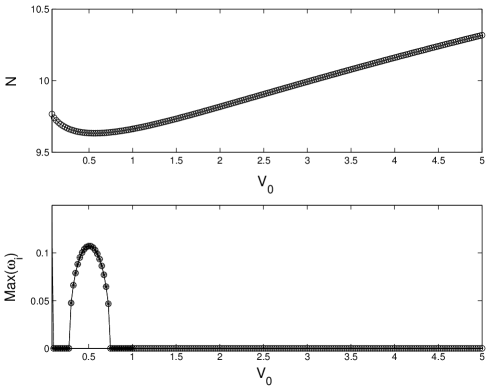
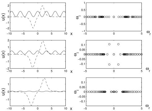
FIG. 1.: Upper part: the top panel shows the number of particles vs. the OL-potential’s strength. The bottom panel shows the largest imaginary part of unstable eigenfrequencies (i.e., the instability growth rate) as a function of $V_{0}$. Lower part: examples of the TLM solutions for $V_{0}=1$ (top panel), $V_{0}=0.5$ (middle panel) and $V_{0}=0.1$ (bottom panel) are shown by dashed curves in the left parts of the panels, while the solid line represents the OL potential. The right panel shows the spectral plane, $\omega_{r},\omega_{i}$), of the real and imaginary parts of the corresponding eigenfrequencies.

Similarly, we examined the evolution of the solutions, setting $V_{0}=1$ and $\mu=-1.5$ in Eq. (3) and performing continuation in $\epsilon$, starting from $\epsilon=0$. In this case too, oscillatory instability was found in a finite interval, $0.05<\epsilon<1.61$. The maximum instability growth rate (which is very large in this case) is $0.48$, and occurs at $\epsilon\approx 0.6$. The results for this case are shown in Fig. 2.

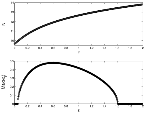
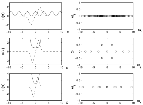
FIG. 2.: The same as Fig. 1, but versus the variation of the parabolic-trap strength $\epsilon$. In the lower part, three examples of the solutions and their stability are given for $\epsilon=0$, $\epsilon=0.6$ and $\epsilon=1.75$.

In these cases, the oscillatory instability arises quite naturally. Indeed, similar instabilities had been observed in the discrete counterpart of the system and, in fact, in the next section we will give a theoretical justification for their occurrence. Another interesting numerical finding is that the TLM solutions appear to be much more robust than one would initially suspect. In particular, there seem to exist TLM solutions even when the OL has been almost completely smeared out by the harmonic trap (see e.g., the last panel of Fig. 2). We will return to this point in the following section.

We also performed the continuation of the TLM solutions with respect to the chemical potential $\mu$, which has yielded results displayed in Fig. 3. In this case, $\epsilon=0$ and $V_{0}=1$ were chosen. The solutions exist in the region $\mu<\mu_{\max}\approx 0.125$. The fact that the cutoff value $\mu_{\max}$ is positive is explained by a contribution of the mean value of the OL potential $V_{0}\cos^{2}x$ in Eq. (3). In this case, oscillatory instability is found in two finite intervals, $-0.375<\mu<-0.1$, and $-0.075<\mu<0$.

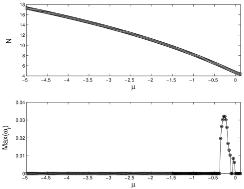
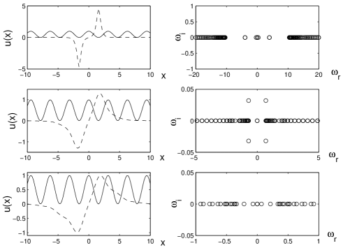
FIG. 3.: The same as in Fig. 1 for the variation with respect to the chemical potential $\mu$. In the lower part, three examples of the TLM solutions correspond to $\mu=-10$ (top), $\mu=-0.25$ (middle) and $\mu=0.125$ (bottom).

B Bound states of two TLM solitons

Complexes which may be considered as a bound state of two TLMs, or simply as a concatenation of three fundamental solitons with phase difference $\pi$ between adjacent ones, were also studied. In this case, for symmetry purposes, $\cos x$ in Eqs. (1) and (3) was replaced by $\sin x$ (recall we have set $\lambda=2\pi$), and three pulses in the initial ansatz (4) were set at $\xi_{j}=-\pi,0,\pi$. We performed the continuation in $\epsilon$, which has demonstrated that the bound state persists to very large values of $\epsilon$, see Fig. 4. The branch becomes unstable, through a quartet of complex eigenfrequencies, at $\epsilon>0.015$. A second instability, accounted for by another eigenvalue quartet, sets in at $\epsilon>0.075$. This second oscillatory instability can be easily explained: as we argue below, for each pair of anti-phase pulses there exists a pair of eigenvalues with negative Krein signature, which is known to give rise to a Hamiltonian Hopf bifurcation [27]. The strongest instability is found at $\epsilon=0.23$, when the two instability growth rates are $0.39$ and $0.35$. The first quartet returns to stability at $\epsilon>0.29$, while the second quartet is stabilized for $\epsilon>0.33$. The bound states are completely stable for $\epsilon>0.33$.

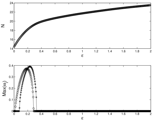
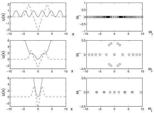
FIG. 4.: The same as in Fig. 2, but for the bound state of two TLM solitons. In the lower part, three examples are shown, for $\epsilon=0$ (top), $\epsilon=0.23$ (middle) and $\epsilon=2$ (bottom panel). Notice that in the second panel of the figure two sets of unstable eigenfrequencies are shown (one by stars and one by circles). This indicates the presence of two unstable eigenvalue quartets, as can also be verified by the spectral plane figure corresponding to the case of $\epsilon=0.23$; see also the discussion in the text.

C Evolution of unstable TLM solitons

In the cases for which the TLM solitons or their bound states were found to be unstable (due to the Hamiltonian Hopf bifurcations), we simulated nonlinear development of the instability in the framework of the full GP equation (1). To this end, a finite-difference scheme with $dx=0.2$ [the same stepsize as in dealing with the stationary equation (3)] was used, and time integration was performed by means of the fourth-order Runge-Kutta scheme with a time step $dt=0.001$. Three examples of the evolution of unstable configurations are shown in Fig. 5. The two top ones correspond, respectively, to the strong and weak oscillatory instability of the TLM soliton. In both of these cases, the TLM state evolves into a single fundamental soliton. A difference between the two cases is that, in the former one, with the relatively weak OL, the newly formed soliton keeps moving between two minima of the potential, while in the latter case , which corresponds to a stronger OL, the fundamental soliton becomes pinned. Finally, the bottom subplot of Fig. 5 demonstrates that the oscillatory instability of a bound state of two TLM solitons transforms it into a single fundamental soliton with a large amplitude.

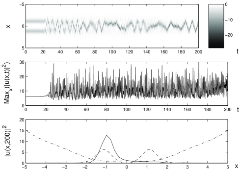
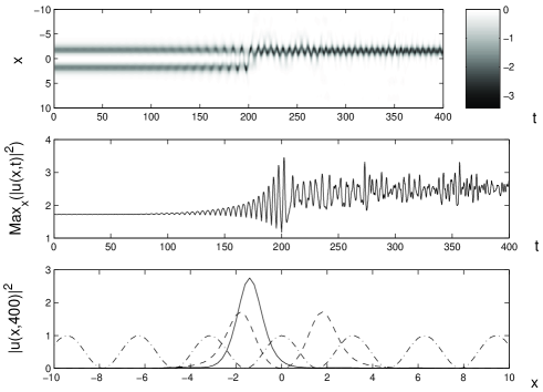
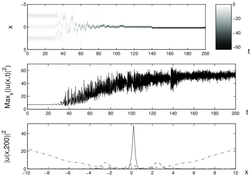
FIG. 5.: Typical examples of the directly simulated evolution of unstable TLM-type solutions. In each set, the top panel displays evolution of the negative local density, $-|u(x,t)|^{2}$ (using a gray-scale space-time plot), the middle panel shows the time evolution of the maximum of $|u(x,t)|^{2}$, and the spatial distribution of the density at the end of the simulation is presented in the bottom panel. In the latter panel, $|u(x,t)|^{2}$ in final and initial states, and the potential are shown, respectively, by solid, dashed, and dashed-dotted lines. The first example is displayed for $\epsilon=0.6$ and $V_{0}=1$; recall that the instability growth rate is $\approx 0.48$ in this case, i.e., it is a case of strong instability. A random-noise perturbation of an amplitude $10^{-5}$ was added to the initial configuration in order to excite the instability. The second example corresponds to $\epsilon=0$ and $V_{0}=1$ for $\mu=-0.25$. As the instability growth rate has a very small value in this case, $0.032$, a random-perturbation seed with a larger amplitude, $\sim 10^{-3}$, was used. The last example pertains to an unstable bound state of two TLM solitons in the case of $\epsilon=0.23$ and $V_{0}=1.0$. In this case, a uniformly distributed random perturbation of amplitude $10^{-5}$ was used to excite the instability.

III Analytical results

A The minimum size of the TLM state

The existence of the TLM state in the GP equation with OL can be explained, by means of perturbation theory, as a bound state of two fundamental solitons with phase difference $\pi$ between them. Here, we consider the case of $\epsilon=0$ (no parabolic trap), but the analysis can be easily generalized to include the trap. If the present model is considered as a perturbed NLS equation, we can use an ansatz in the form of Eq. (4) for two solitons. The system’s Hamiltonian reads

$\displaystyle H=\int_{-\infty}^{\infty}\left[|u_{x}|^{2}-\frac{1}{2}|u|^{4}+V_{0}\cos^{2}\left(\frac{2\pi x}{\lambda}\right)|u|^{2}\right]dx.$

Recall that we have set $\epsilon=0$; here, for generality’s sake, we do not fix $\lambda=2\pi$. Then, known methods (see a review in Ref. [28]) yield an effective net potential of the interaction between two solitons and interaction of both solitons with the OL. This potential is realized as a part of the Hamiltonian that depends on the coordinates $\xi_{1}$ and $\xi_{2}$ of the solitons and phase difference $\Delta\phi$ between them (cf. a similar potential for solitons in the discrete-NLS model found in Ref. [22]) and is of the form:

$$V_{{\rm eff}}\left(\xi_{1},\xi_{2};\Delta\phi\right) = -8\eta^{3}\cos\left(\Delta\phi\right)\exp\left(-\frac{\eta}{\sqrt{2}}\left|\xi_{1}-\xi_{2}\right|\right)$$ (7)

$$+\frac{2\sqrt{2}\pi^{2}V_{0}}{\lambda\sinh\left(\frac{2\sqrt{2}\pi^{2}}{\lambda\eta}\right)}\left[\cos\left(\frac{4\sqrt{2}\pi}{\lambda}\xi_{1}\right)+\cos\left(\frac{4\sqrt{2}\pi}{\lambda}\xi_{2}\right)\right].$$

The second term in this expression is the Peierls-Nabarro potential (see, e.g., Ref. [25] and references therein) induced by the OL. Equilibrium positions of the two-soliton system are determined by equations

$$\frac{\partial V_{{\rm eff}}}{\partial\xi_{1}}=\frac{\partial V_{{\rm eff}}}{\partial\xi_{2}}=\frac{\partial V_{{\rm eff}}}{\partial\left(\Delta\phi\right)}=0.$$ (8)

Straightforward consideration of Eqs. (8) and (7) shows that a bound state of two solitons with $\Delta\phi=\pi$, which corresponds to a TLM-like pattern, may exist if the separation $L\equiv\left|\xi_{1}-\xi_{2}\right|$ between them exceeds the minimum value,

$$L_{\min}=\frac{\sqrt{2}}{\eta}\ln\left[\frac{\lambda^{2}\eta^{4}}{\sqrt{2}\pi^{3}V_{0}}\sinh\left(\frac{2\sqrt{2}\pi^{2}}{\lambda\eta}\right)\right].$$ (9)

This prediction for the minimum separation between fundamental-soliton components of the TLM state was tested numerically. As a typical example, in Fig. 6 we show the variation of $L_{\min}$ with $V_{0}$ for $\lambda=2\pi$ and $\eta=\sqrt{3}$. The distance between the centers of the solitons was extracted from numerical data as the distance between two local maxima of $\left|u(x)\right|$, an inherent discretization error of $\pm 0.2$ being imposed by the finite-difference scheme. As is seen, the agreement between the theoretical prediction and the numerically approximated values of $L_{\min}$ is quite good.

A more detailed analytical consideration of dynamical properties of a perturbed bound state (following the lines of Ref. [22]) shows that, within the framework of the present approximation, the bound state is stable. Moreover, the existence of stable bound states of three fundamental solitons, which correspond to the bound state of two TLMs considered above, can also be demonstrated by means of this approach.

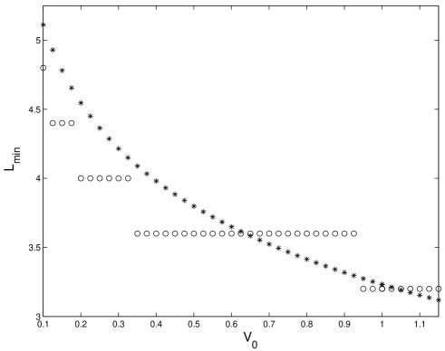
FIG. 6.: The analytical prediction (9) for the minimum separation between two $\pi$-out-of-phase fundamental solitons in the bound state (stars), and the separation between two density maxima in the TLM found from numerical data (circles), versus $V_{0}$. Notice that the numerical results should be considered with an error bar of $\pm 0.2$, due to the discretization used.

B Oscillatory instabilities of the single-TLM and double-TLM states

It is well known (see e.g., Ref. [25] and references therein) that the linearized equations for the perturbations defined in Eq. (5) can be rewritten, in terms of new variables $U=a+b^{\ast}$ and $W=a-b^{\ast}$, as

$$\omega U = L_{-}W\equiv-W_{xx}-v^{2}W+(V(x)-\mu)W,$$ (10)

$$\omega W = L_{+}U\equiv-U_{xx}-3v^{2}U+(V(x)-\mu)U_{n}.$$ (11)

The Krein signature of the eigenvalue can be written as [26]

$\displaystyle K={\rm sign}\left(-\int_{-\infty}^{\infty}(UW^{\star}+WU^{\star})dx\right).$

Analytical consideration is possible for $\omega$’s that are real; then $U$ and $W$ are also real, hence $K$ amounts to the expression

$$K={\rm sign}\left(-\int_{-\infty}^{\infty}UWdx\right).$$ (12)

As was done above, we approximate a TLM solution as a superposition, $v(x)=P(x)+N(x)$, of two stationary fundamental-soliton waveforms, positive $P(x)$ and negative $N(x)$, the underlying assumption being a weak overlap between $P(x)$ and $N(x)$. Since $P$ and $N$ are, essentially, individual solitons, in the lowest-order approximation they obey equations $\left[V(x)-\mu\right]P=P_{xx}+P^{3}$ and $\left[V(x)-\mu\right]N=N_{xx}+N^{3}$. Summing them up, and taking into account that the product $\left|PN\right|$ is everywhere much smaller than $P^{2}+N^{2}$ (due to the assumed weak overlap between $P$ and $N$), we conclude that, up to the same lowest-order accuracy, the function $P(x)+N(x)$ satisfies the equation $L_{-}(P+N)=0$ [recall that the operator $L_{-}$ is defined in Eq. (10)]. Thus, in the lowest approximation, $P(x)+N(x)$ is a zero mode of the operator $L_{-}$. In a similar way, the following approximate result can be obtained for the function $P(x)-N(x)$:

$$L_{-}(P-N)=-PN(P-N).$$ (13)

The linearization around each of the TLM-constituent pulses (if considered in isolation) carries a pair of zero eigenvalues due to the phase invariance. The corresponding eigenfunction, $W$, has the shape of the pulse itself ($P$ and $N$, respectively). There is also a generalized eigenfunction [26] for each pair. We expect to have two pairs of TLM eigenvalues originating from these pairs of the individual-soliton’s ones, the corresponding eigenfunctions being (in the lowest approximation) $W=P+N$ and $W=P-N$. The former one is related to the phase invariance of the system (in other words, to the conservation of the total number of atoms), which means that the corresponding eigenvalue pair remains exactly equal to zero, while the other one may become different than zero. Then, it follows from Eq. (13) and Eq. (10) that, in the lowest approximation, $U=-PN(P-N)$. In turn, Eq. (12) yields

$$K={\rm sign}\left[\int_{-\infty}^{\infty}PN(P-N)^{2}dx\right].$$ (14)

Since, by definition, the signs of $P(x)$ and $N(x)$ are opposite, Eq. (14) implies that the Krein signature of this phase eigenmode is negative. A known consequence of this [27] is that an oscillatory instability will be generated by collision of this nonzero eigenvalue with other discrete ones (and/or those belonging to the continuous spectrum) that carry a positive Krein signature.

The above consideration indicates that, for every pair of the interacting $\pi$-out-of-phase pulses, there exists an eigenvalue with negative Krein signature and, consequently, a potentially ensuing Hamiltonian Hopf bifurcation. This conclusion fully agrees with our numerical results presented above, that have identified a single oscillatory instability for the single TLM soliton, and two such instabilities in the case of bound states of two TLM solitons.

C TLM solitons in the absence of the OL

Finally, it is possible to present analytical arguments justifying the existence of TLM solitons (both single and multiple ones) even when the harmonic trap is overwhelmingly stronger than the OL potential (see the numerical results shown in the last panels in Figs. 2 and 4), or when the OL potential is simply absent. Within the framework of the same perturbation theory which was employed above to derive Eq. (7), each of the pulses constituting the TLM state is then subject to the action of two forces. One of them is exerted by the magnetic trap, while the other comes from the interaction between the pulses. Accordingly, the effective potential is

$$V_{{\rm eff}}(\xi_{1},\xi_{2};\Delta\phi) = -8\eta^{3}\cos\left(\Delta\phi\right)\exp\left(-\frac{\eta}{\sqrt{2}}\left|\xi_{1}-\xi_{2}\right|\right)$$ (16)

$$+4\sqrt{3}\epsilon\left(\xi_{1}^{2}+\xi_{2}^{2}\right).$$

Predictions following from this approximation were tested against direct numerical results obtained in the absence of the OL, i.e., with $V_{0}=0$ in Eq. (1). In Fig. 7, an example is displayed for $\epsilon=0.2$ and $\mu=-1.5$. The top panel shows the effective potential (16), which, in this case, has a minimum at $\xi_{1,2}=\pm 1.35$. The middle and bottom panels present a numerical solution, with maxima of $\left|u(x)\right|$ at $\xi_{1,2}\approx\pm 1.4$. Thus, the perturbative approximation not only explains the existence of the TLM state in attractive BECs even in the absence of OL, but also accurately predicts the location of centers of the pulses whose concatenation generates the TLM structure. This, in turn, supports the numerical findings presented in section II, which suggested that TLM solitons in the attractive BEC would indeed persist even for very tight magnetic traps. Thus, we conclude that the TLM solitons are a very robust feature of the system.

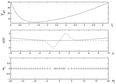
FIG. 7.: The top panel shows the effective potential $V_{{\rm eff}}$, as a function of the coordinate $\xi$ of the right pulse, which is induced by the repulsion between the pulses and the restoring force from the magnetic trap, following the analytical expression (16). The potential minimum (equilibrium position) is located at $\xi\approx 1.35$. The middle and bottom panels show the TLM configuration and its stability, as found in the numerical form. The equilibrium position corresponding to the numerical solution is inferred from the middle plot to be at $\xi\approx 1.4$. The parameters are $V_{0}=0$, $\epsilon=0.2$, and $\mu=-1.5$.

IV Conclusions

In this work we have demonstrated that counterparts of twisted localized modes (TLMs), which were earlier found in the discrete one-dimensional NLS equation, can exist as robust objects in attractive, effectively one-dimensional Bose-Einstein condensates (BECs), provided that the condensate is confined by the optical lattice (OL) and/or parabolic magnetic trap. The TLMs in BECs may be considered as bound states of two fundamental solitons with a phase difference $\pi$ between them, or, alternatively, as a dark soliton embedded in a broader bright one. The family of the TLM solitons and their stability were investigated in detail, by means of numerical continuation in the strengths of the OL or magnetic-trap parameters, as well as in the chemical potential. Stable bound states of two TLMs, alias a bound state of three fundamental solitons with a $\pi$ phase shift between adjacent ones, were also found. In the cases when the TLMs are unstable, the development of the instability was monitored by means of direct simulations, with a conclusion that the TLM rearranges itself into a fundamental soliton.

We have also developed an analytical approach, which treats each fundamental soliton as a quasi-particle subject to the action of effective forces exerted by the OL, magnetic trap, and interaction with another soliton. The analysis predicts the existence of the stable bound state of two fundamental solitons with a phase shift of $\pi$ between them. The smallest possible distance between the bound solitons, predicted by this approach, is in good agreement with the numerically found size of the corresponding TLM. The analysis can be readily extended to predict that multi-pulse bound states with the phase shift $\pi$ between adjacent solitons also exist and may be stable.

The origin of the instability of the TLMs, in the case when they are unstable, was also examined by means of an analytical approximation, and was found to stem from Hamiltonian Hopf bifurcations, which occur when eigenvalues with negative Krein signature collide with positive-signature ones. This result was based on the existence of a negative-Krein-sign eigenvalue set, that was constructed by means of the perturbative analysis.

It will be very interesting to generalize these considerations to higher dimensions – in particular to two-dimensional settings. In that case, a relevant issue is the possible existence of a 2D counterpart of the TLM in the form of a bright vortex (which was found in the 2D discrete NLS equation, where it was shown to be stable under certain conditions [29]). A very recent preliminary result is that bright vortices, stabilized by a 2D optical lattice, can indeed be found [30].

REFERENCES

- [1] F. Dalfovo, S. Giorgini, L.P. Pitaevskii, and S. Stringari, Rev. Mod. Phys. 71, 463 (1999).
- [2] S. Burger et al., Phys. Rev. Lett. 83, 5198(1999); J. Denschlag et al., Science 287, 97 (2000); B.P. Anderson et al., Phys. Rev. Lett. 86, 2926 (2001).
- [3] K.E. Strecker, G.B. Partridge, A.G. Truscott, and R.G. Hulet, Nature 417, 150 (2002); L. Khaykovich, F. Schreck, G. Ferrari, T. Bourdel, J. Cubizolles, L.D. Carr, Y. Castin, and C. Salomon, Science 296, 1290 (2002).
- [4] M.R. Matthews et al., Phys. Rev. Lett. 83, 2498(1999); K.W. Madison, et al. Phys. Rev. Lett. 84, 806 (2000); S. Inouye et al., Phys. Rev. Lett.87, 080402 (2001).
- [5] K. Staliunas, S. Longhi and G. J. de Valcárcel, Phys. Rev. Lett. 89, 210406 (2002).
- [6] G. Theocharis, D.J. Frantzeskakis, P.G. Kevrekidis, B.A. Malomed and Yu.S. Kivshar, “Ring dark solitons and vortex necklaces in Bose-Einstein condensates”, e-print cond-mat/0302102; Phys. Rev. Lett., in press.
- [7] S. Inouye et al., Nature 392, 151 (1998); E.A. Donley et al., Nature 412, 295 (2001).
- [8] P.J.Y. Louis, E.A. Ostrovskaya, C.M. Savage and Yu.S. Kivshar, Phys. Rev. A 67, 013602 (2003).
- [9] S. Darmanyan, A. Kobyakov and F. Lederer, Sov. Phys. JETP 86, 682 (1998); P.G. Kevrekidis, A.R. Bishop and K.Ø. Rasmussen, Phys. Rev. E 63, 036603 (2001).
- [10] A.J. Moerdijk, W.C. Stwalley, R.G. Hulet, and B.J. Verhaar, Phys. Rev. Lett. 72, 40 (1994).
- [11] J.P. Burke, J.L. Bohn, B.D. Esry, and C.H. Greene, Phys. Rev. Lett. 80, 2097 (1998).
- [12] B.B. Baizakov, V.V. Konotop and M. Salerno, J. Phys. B 35, 5105 (2002); K.M. Hilligsoe, M.K. Oberthaler, and K.P. Marzlin, Phys. Rev. A 66, 063605 (2002); E.A. Ostrovskaya and Y.S. Kivshar, e-print cond-mat/0303190 (2003).
- [13] P.A. Ruprecht, M.J. Holland, K. Burnett and M. Edwards, Phys. Rev. A 51, 4704 (1995).
- [14] V.M. Pérez-García, H. Michinel and H. Herrero, Phys. Rev. A 57, 3837 (1998); L. Salasnich, A. Parola and L. Reatto,Phys. Rev. A 65, 043614 (2002); Y.B. Band, I. Towers, and B.A. Malomed, Phys. Rev. A 67, 023602 (2003).
- [15] F.S. Cataliotti, S. Burger, C. Fort, P. Maddaloni, F. Minardi, A. Trombettoni, A. Smerzi and M. Inguscio, Science 293, 843 (2001).
- [16] M. Greiner, I. Block, O. Mandel, T.W. Hänsch and T. Esslinger, Appl. Phys. B 73, 769 (2001).
- [17] A. Trombettoni and A. Smerzi, Phys. Rev. Lett. 86, 2353, (2001).
- [18] F.Kh. Abdullaev, B.B. Baizakov, S.A. Darmanyan, V.V. Konotop, and M. Salerno, Phys. Rev. A64, 043606 (2001).
- [19] A. Smerzi, A. Trombettoni, P.G. Kevrekidis, and A.R. Bishop Phys. Rev. Lett. 89, 170402 (2002).
- [20] F. S. Cataliotti, L. Fallani, F. Ferlaino, C. Fort, P. Maddaloni, M. Inguscio, A. Smerzi, A. Trombettoni, P. G. Kevrekidis, A. R. Bishop, “A Novel mechanism for superfluidity breakdown in weakly coupled Bose-Einstein condensates”, e-print cond-mat/0207139.
- [21] For finite difference schemes for partial differential equations the interested reader can be referred to e.g., G.D. Smith, Numerical Solution of Partial Differential Equations: Finite Difference Methods, Oxford University Press (Oxford, 1986); G.E. Forsythe and W.R. Wasow, Finite-Difference Methods for Partial Differential Equations, John Wiley & Sons, Inc. (New York, 1960). For Newton type methods, as well as finite difference schemes, one can consult: W.H. Press et al., Numerical Recipes in C: The Art of Scientific Computing, Cambridge University Press (Cambridge, 1988).
- [22] T. Kapitula, P.G. Kevrekidis and B.A. Malomed, Phys. Rev. E 63, 036604 (2001).
- [23] J.C. Bronski et al. Phys. Rev. Lett. 86, 1402 (2001); J.C. Bronski et al. Phys. Rev. E 64, 056615 (2003).
- [24] Matlab, The Language of Scientific Computing, the Mathworks Inc., Natick, MA (2000).
- [25] P.G. Kevrekidis, K.Ø. Rasmussen and A.R. Bishop, Int. J. Mod. Phys. B 15, 2833 (2001).
- [26] M. Johansson and S. Aubry, Phys. Rev. E 61, 5864 (2000).
- [27] J.-C. van der Meer, Nonlinearity 3, 1041 (1990); see also e.g., I.V. Barashenkov, D.E. Pelinovsky and E.V. Zemlyanaya, Phys. Rev. Lett. 80, 5117 (1998); A. De Rossi, C. Conti and S. Trillo, Phys. Rev. Lett. 81, 85 (1998); M. Johansson and Yu.S. Kivshar, Phys. Rev. Lett. 82, 85 (1999).
- [28] B.A. Malomed, Progr. Optics 43, 71 (2002).
- [29] B.A. Malomed and P.G. Kevrekidis, Phys. Rev. E 64, 026601 (2001).
- [30] B. Baizakov, B.A. Malomed, and M. Salerno, in preparation.