The Grover algorithm with large nuclear spins in semiconductors

Abstract

We show a possible way to implement the Grover algorithm in large nuclear spins $1/2<I\leq 9/2$ in semiconductors. The Grover sequence is performed by means of multiphoton transitions that distribute the spin amplitude between the nuclear spin states. They are distinguishable due to the quadrupolar splitting, which makes the nuclear spin levels non-equidistant. We introduce a generalized rotating frame for an effective Hamiltonian that governs the non-perturbative time evolution of the nuclear spin states for arbitrary spin lengths $I$. The larger the quadrupolar splitting, the better the agreement between our approximative method using the generalized rotating frame and exact numerical calculations.

]

I Introduction

Recent experiments[1, 2] have shown that electron spins in GaAs can preserve their coherence for distances of more than 100 $\mu$m and for times of up to 130 ns. Long coherence lengths and times are the main requirement for performing logic operations in spintronics[3, 4, 5, 6, 7] and quantum computing,[5, 8, 9, 10, 11, 12, 13, 14, 15, 16] because both research fields are interested in the complete control over the phase information of the spins and qubits, respectively. Among the various available information carriers, nuclear spins have one of the longest coherence times due to their weak interaction with the environment. which amounts to storing phase information for a long time in e.g. semiconductor structures. Either they can be used as qubits or in the unary representation.[17] Although implementations based on the latter are not scalable, they are more feasible, more robust, and can also be implemented in classical systems.[18] Coherent access to the nuclear spins in semiconductors is achieved by the all-optical NMR method shown in Refs. [19] and [20], which makes use of the hyperfine interaction between the electron and nuclear spins and relies on the large coherence time of the electrons. A further possibility to access the nuclear spins coherently is conventional NMR using coils.[21] However, compared to the all-optical method, coils do not provide the spatially selective manipulation of nuclear spins. Recently incoherent transfer of electronic spin to nuclear spin has been demonstrated experimentally in semiconductor structures using the quantum Hall effect or ferromagnetic imprinting.[22, 23]

One of the most interesting quantum algorithms was introduced by Grover,[24] who demonstrated that the parallelism of unitary operations can speed up the search for a desired quantum state. Since the Grover algorithm needs only the superposition principle of quantum or classical mechanics, the unary representation of an ensemble of single particles can be used, such as the atomic levels of a beam of atoms[25] or the large spin of molecular magnets embedded in a crystal.[26] In this paper we show that the NMR method presented in Ref. [17] works for arbitrary spin lengths $I$. We compute the Grover algorithm on the single-spin states $\left|m\right>$ of the large spin of nuclear spins in semiconductors. For this it is essential that a delocalized state $\left|\psi\right>=\sum_{m=-I}^{I}a_{m}\left|m\right>$ with arbitrary amplitudes $a_{m}$ can be produced, which we show to be feasible with a single magnetic rf pulse. Since arbitrary amplitudes $a_{m}$ are needed, we derive a non-perturbative method to calculate the time evolution of the nuclear spins that is valid for arbitrary spin lengths $I$. We also perform exact numerical calculations based on solving the Schrödinger equation. It turns out that the larger the quadrupolar splitting, the better the agreement between our non-perturbative method and the exact numerical calculations. In order to be able to control the nuclear spins coherently, the energy levels $\varepsilon_{m}$ have to be non-equidistant, which is ensured by the quadrupolar splitting. Instead of encoding the information into the phases of $a_{m}$, we encode the information into the eigenenergies $\delta_{I-m}$ of the eigenstates $\left|m\right>$ in the generalized rotating frame (see below).[27, 28] After choosing a specific basis state $\left|M\right>$ to be looked for, we make it degenerate with the completely delocalized state $\left|s\right>=\sum_{m=-I}^{I}a_{m}\left|m\right>$ that has equal amplitudes $a_{m}$ in the generalized rotating frame, i.e. a second magnetic rf pulse lets $\left|s\right>$ evolve into $\left|M\right>$, which is ensured by the finite overlap of $\left|s\right>$ and $\left|M\right>$.

In Sec. II we give the Hamiltonian that is the most suitable for nuclear spins in semiconductors. For the time evolution of the nuclear spins we first identify the transition (Feynman) diagrams that give the largest contribution to the multiphoton transition amplitudes by means of high-order time-dependent perturbation theory, which is demonstrated in Sec. III. From this we derive effective Hamiltonians in the so-called generalized rotating frame that describe the time evolution of the nuclear spins non-perturbatively for arbitrary spin lengths $I$, which is shown in Sec. V. In order to understand better our concept of the generalized rotating frame in Sec. V, we first review the transformation to the standard rotating frame in Sec. IV. In Sec. VI we explain our proposed method to implement the Grover algorithm into the single-spin system of nuclei in semiconductors. Finally, Sec. VII shows that conventional incoherent NMR can be used to read out the searched state after performing the Grover quantum search algorithm.

FIG. 1.: Multiphoton transition scheme (QC scheme) for the coherent population of the $I_{z}$ eigenstates $\left|m\right>$ of a nuclear spin $I=3/2$. In this scheme the Grover algorithm can be implemented non-perturbatively. The frequencies $\omega_{k}$ of the fields $H_{k}$ are red (- $\cdot$) and blue (- -) detuned. Diagrams containing blue detunings are negligible for large quadrupolar splitting, i.e. $A\gg\hbar\delta_{k}\geq 0$. In Sec. III we explain why only the leftmost diagram is relevant.

II Model Hamiltonian

The ensemble of nuclear spins in semiconductors is best described by the single-spin Hamiltonian

$${\cal H}_{0}={\cal H}_{\rm Z}+{\cal H}_{\rm Q},$$ (1)

which consists of the nuclear Zeeman term

$${\cal H}_{\rm Z}=-g_{N}\mu_{N}H_{z}I_{z},$$ (2)

with the nuclear $g$-factor $g_{N}=1.3$ (see Ref. [19]), and the quadrupolar term[21]

$${\cal H}_{\rm Q}=A[3I_{z}^{2}-I(I+1)].$$ (3)

The quadrupolar constant $A$ differs significantly between the various nuclei. For example the all-optical NMR method shown in Ref. [20] yields the following quadrupolar constants for Ga and As nuclei in GaAs semiconductors: $A=7\times 10^{-7}$ K for ⁶⁹Ga, $A=3\times 10^{-7}$ K for ⁷¹Ga, and $A=2\times 10^{-6}$ K for ⁷⁵As. Let $\left|m\right>$ be the eigenstates of ${\cal H}_{0}$ with eigenenergies $\varepsilon_{m}$.

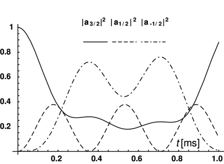
FIG. 2.: Preparation of $\left|s\right>=(1/\sqrt{3})\sum_{m=-1/2}^{3/2}\left|m\right>$ by means of Eq. (95) in the QC scheme, which takes about 0.2 ms for $H_{1}=H_{2}=1$ G, $H_{3}=0$, $\delta_{1}=6083$ s^-1, and $\delta_{2}=0$. The analytical result is confirmed by numerics in Fig. 3. The calculation was done in the generalized rotating frame as described in Sec. V.

Next, we apply external magnetic fields $H_{x,k}(t)=\tilde{H}_{k}(t)\cos(\omega_{k}t+\Phi_{k})$, $k=1,2,3,\ldots$, that differ by the phases $\Phi_{k}$ and oscillate at frequencies $\omega_{k}$ being detuned by $\delta_{k}$ from the differences between the energy levels $\varepsilon_{m}$. To be more precise, $\omega_{k}$ is detuned by $\delta_{k}$ from $\varepsilon_{2I-k+1}-\varepsilon_{2I-k}$. Fig. 1 shows the example for $I=3/2$ and $k=1,2,3$. If $\delta_{k}<0$ the detuning is said to be blue, and if $\delta_{k}>0$ the detuning is said to be red. For GaAs, $\omega_{k},\omega_{k}^{\prime}\sim 10$ MHz with $\delta_{k}\sim 1$ kHz, and a longitudinal magnetic field $H_{z}\sim 1$ T is appropriate. It is desirable to make $H_{z}$ sufficiently large to accommodate many spin precessions before the spins dephase. The complete Hamiltonian has then the form

$${\cal H}={\cal H}_{0}+V(t),$$ (4)

where

$$V(t)=\sum_{k=1}^{2I}g_{N}\mu_{N}\tilde{H}_{k}(t)\cos(\omega_{k}t+\Phi_{k})I_{x}$$ (5)

is the driving Hamiltonian given by the external magnetic fields. As usual, the spin operator can be decomposed into ladder operators, i.e. $I_{x}=(I_{+}+I_{-})/2$.

For the implementation of the non-perturbative version of the Grover algorithm[27, 28] we have to be able to produce a completely delocalized state of the form $\left|\psi\right>=\sum_{m=-I}^{I}a_{m}\left|m\right>$ with arbitrary amplitudes $a_{m}$. Furthermore, we need to have coherent control over the unitary time evolution of $\left|\psi(t)\right>$ for arbitrary times $t$. We will show in the next sections that our non-perturbative method gains complete control over all the amplitudes $a_{m}(t)$, which can be used in a future experimental implementation.

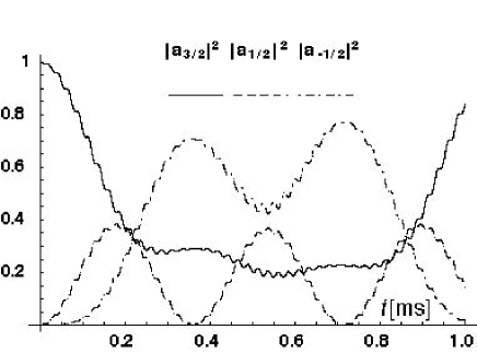
FIG. 3.: Preparation of $\left|s\right>=(1/\sqrt{3})\sum_{m=-1/2}^{3/2}\left|m\right>$ by solving the Schrödinger equation exactly for ⁷¹Ga nuclei in the QC scheme, which takes about 0.2 ms for $H_{1}=H_{2}=1$ G, $H_{3}=0$, $\delta_{1}=6083$ s^-1, and $\delta_{2}=0$. The small oscillations are due to the five diagrams with blue detunings (see Fig. 1) that have been neglected in Fig. 2. The ⁷¹Ga nuclei have an anisotropy constant of $A=3\times 10^{-7}$ K.

III Perturbative expansion

Usually perturbation theory is useful only if the transverse term $V(t)$ is small compared to the longitudinal term ${\cal H}_{0}$. But here we use high-order time-dependent perturbation theory to identify the transition diagrams with the largest contribution to the transition amplitudes $S_{m,m^{\prime}}=\lim_{t\rightarrow-\infty,t^{\prime}\rightarrow\infty}\left<m\left|U(t,t^{\prime})\right|m^{\prime}\right>$. For this we first expand the $S$-matrix in powers of $V(t)$, i.e. $S=\sum_{j=0}^{\infty}S^{(j)}$. The $j$th-order term of the perturbation series of the $S$-matrix in powers of the driving Hamiltonian $V(t)$ is expressed by

$$S^{(j)} = \left(\frac{1}{i\hbar}\right)^{j}\prod_{k=1}^{j-1}\int_{-\infty}^{\infty}dt_{k}\int_{-\infty}^{\infty}dt_{j}\Theta(t_{k}-t_{k+1})U_{0}(\infty,t_{1})$$ (7)

$$\times V(t_{1})U_{0}(t_{1},t_{2})V(t_{2})\ldots V(t_{j})U_{0}(t_{j},-\infty),$$

which corresponds to the sum over all transition diagrams of order $j$, and where $U_{0}(t,t_{0})=e^{-i{\cal H}_{0}(t-t_{0})/\hbar}$ is the free propagator, $\Theta(t)$ is the Heavyside function.

For illustration, we derive now a three $\sigma$-photon transition from $\left|3/2\right>$ to $\left|-3/2\right>$. All the relative phases $\Phi_{k}$ between the magnetic fields are assumed to be zero in this calculation. Then we obtain

$$S_{-\frac{3}{2},\frac{3}{2}}^{(3)} = \left(\frac{g\mu_{N}}{4i\hbar}\right)^{3}\int\!\int\!\int dt_{1}dt_{2}dt_{3}\Theta(t_{1}-t_{2})\Theta(t_{2}-t_{3})$$ (10)

$$\times p_{-\frac{3}{2},\frac{3}{2}}e^{i\varepsilon_{\frac{3}{2}}t_{1}/\hbar}e^{-i\varepsilon_{\frac{1}{2}}(t_{1}-t_{2})/\hbar}e^{-i\varepsilon_{-\frac{1}{2}}(t_{2}-t_{3})/\hbar}$$

$$\times e^{-i\varepsilon_{-\frac{3}{2}}t_{3}/\hbar}\prod_{l=1}^{3}\sum_{k=1}^{3}\tilde{H}_{k}(t_{l})\left(e^{i\omega_{k}t_{l}}+e^{-i\omega_{k}t_{l}}\right)$$

$$\approx \left(\frac{g\mu_{N}}{4i\hbar}\right)^{3}\int\!\int\!\int dt_{1}dt_{2}dt_{3}\Theta(t_{1}-t_{2})\Theta(t_{2}-t_{3})$$ (13)

$$\times p_{-\frac{3}{2},\frac{3}{2}}\tilde{H}_{3}(t_{1})\tilde{H}_{2}(t_{2})\tilde{H}_{1}(t_{3})e^{i(\omega_{-\frac{3}{2},\frac{3}{2}}-\omega_{1}-\omega_{2}-\omega_{3})t_{1}}$$

$$\times e^{-i(\omega_{-\frac{1}{2},\frac{3}{2}}-\omega_{1}-\omega_{2})(t_{1}-t_{2})}e^{-i(\omega_{\frac{1}{2},\frac{3}{2}}-\omega_{1})(t_{2}-t_{3})}$$

where from the $3^{3}=27$ terms remains only one due to the rotating wave approximation and after keeping only the terms with the smallest detuning. This diagram is the most left one in Fig. 1.

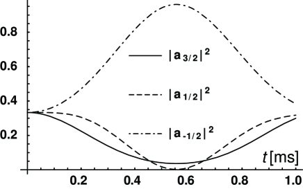
FIG. 4.: Grover algorithm calculated by means of Eq. (95) in the QC scheme, where $\left|s\right>=(1/\sqrt{3})\sum_{m=-1/2}^{3/2}\left|m\right>$ is concentrated mainly into $\left|-1/2\right>$ after 0.55 ms for $H_{2}=\hbar\delta_{2}/2g_{N}\mu_{N}=1$ G, $h_{1}=h_{2}$, $h_{3}=0$, $\delta_{1}=0$. The duration of the QC is $\leq 1/2\nu_{\rm Rabi}^{(2)}$. This result is numerically confirmed in Fig. 5. The calculation was done in the generalized rotating frame as described in Sec. V.

Next, we make use of the relation

$$e^{-i(\omega_{m,m^{\prime}}-\omega)(t-t^{\prime})}\Theta(t-t^{\prime}) = \frac{i}{2\pi}\int_{-\infty}^{\infty}d\Omega$$ (15)

$$\times\frac{e^{-i\Omega(t-t^{\prime})}}{\Omega-\omega_{m,m^{\prime}}+\omega+i\varepsilon}$$

and substitute the Fourier transform

$$\tilde{H}(\Omega)=\frac{1}{\sqrt{2\pi}}\int_{-\infty}^{\infty}\tilde{H}(t)e^{i\Omega t}dt,$$ (16)

which yields

$$S_{-\frac{3}{2},\frac{3}{2}}^{(3)} \approx \left(\frac{g\mu_{N}}{4\hbar}\right)^{3}\frac{p_{-\frac{3}{2},\frac{3}{2}}}{\sqrt{2\pi}i}\int\!\int d\Omega d\Omega^{\prime}\frac{\tilde{H}_{2}(\Omega-\Omega^{\prime})\tilde{H}_{3}(\Omega^{\prime})}{\Omega^{\prime}-\omega_{\frac{1}{2},\frac{3}{2}}+\omega_{1}+i\varepsilon}$$ (18)

$$\times\frac{\tilde{H}_{1}(\omega_{-\frac{3}{2},\frac{3}{2}}-\omega_{1}-\omega_{2}-\omega_{3}-\Omega)}{\Omega-\omega_{-\frac{1}{2},\frac{3}{2}}+\omega_{1}+\omega_{2}+i\varepsilon}$$

$$\approx \left(\frac{g\mu_{N}}{4\hbar}\right)^{3}\frac{p_{-\frac{3}{2},\frac{3}{2}}}{\sqrt{2\pi}i}\int\!\int d\Omega d\Omega^{\prime}\frac{\tilde{H}_{2}(\Omega-\Omega^{\prime})\tilde{H}_{1}(\Omega^{\prime})}{\omega_{\frac{1}{2},\frac{3}{2}}+\omega_{1}}$$ (20)

$$\times\frac{\tilde{H}_{3}(\omega_{-\frac{3}{2},\frac{3}{2}}-\omega_{1}-\omega_{2}-\omega_{3}-\Omega)}{\omega_{-\frac{1}{2},\frac{3}{2}}+\omega_{1}+\omega_{2}},$$

as long as all $\tilde{H}_{k}(\Omega)$ have a sufficiently narrow peak around $\Omega=0$ and $\omega_{k}$ are detuned.

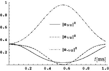
FIG. 5.: Grover algorithm calculated by solving the Schrödinger equation exactly for ⁷⁵As nuclei in the QC scheme, where $\left|s\right>=(1/\sqrt{3})\sum_{m=-1/2}^{3/2}\left|m\right>$ is concentrated mainly into $\left|-1/2\right>$ after 0.55 ms for $H_{2}=\hbar\delta_{2}/2g_{N}\mu_{N}=1$ G, $h_{1}=h_{2}$, $h_{3}=0$, $\delta_{1}=0$. The ⁷⁵As nuclei have an anisotropy constant of $A=2\times 10^{-6}$ K, which is about 10 times larger than for ⁷¹Ga nuclei. Therefore the small oscillations due to the neglected five diagrams in Fig. 1 are here almost invisible. Hence we can infer that the larger the quadropular constant $A$, the better the agreement between our non-perturbative method and exact numerics.

After evaluation of the three-fold convolution we obtain

$$S_{-\frac{3}{2},\frac{3}{2}}^{(3)} \approx \left(\frac{g\mu_{N}}{4\hbar}\right)^{3}\frac{\int dt\prod_{k=1}^{3}\tilde{H}_{k}(t)e^{i(\omega_{-\frac{3}{2},\frac{3}{2}}-\omega_{1}-\omega_{2}-\omega_{3})t}}{ip_{-\frac{3}{2},\frac{3}{2}}^{-1}(\omega_{1}-\omega_{\frac{1}{2},\frac{3}{2}})(\omega_{1}+\omega_{2}-\omega_{-\frac{1}{2},\frac{3}{2}})}$$ (21)

$$= \left(\frac{g\mu_{N}}{4\hbar}\right)^{3}\frac{\prod\limits_{k=1}^{3}H_{k}\delta^{(T)}(\omega_{-\frac{3}{2},\frac{3}{2}}-\omega_{1}-\omega_{2}-\omega_{3})}{i(2\pi p_{-\frac{3}{2},\frac{3}{2}})^{-1}\delta_{1}\delta_{2}},$$ (22)

where $p_{m,m^{\prime}}=\prod_{k=m}^{m^{\prime}}\left<k\left|I_{-}\right|k+1\right>$ is the spin amplitude between $\left|k\right>$ and $\left|k+1\right>$ and $\delta^{(T)}(\omega)=\frac{1}{2\pi}\int_{-T/2}^{+T/2}e^{i\omega t}dt=\frac{\sin(\omega T/2)}{\pi\omega}$ is the delta-function of width $1/T$. In addition, we have used rectangular pulse shapes of duration $T$ for all fields, i.e.

$$\tilde{H}_{k}(t)=\left\{\begin{array}[]{l}H_{k}\text{ for }-T/2<t<T/2,\\ 0\text{ otherwise}.\end{array}\right.$$ (23)

The energy is conserved for $\omega T\gg 1$. Also, the duration $T$ of the rf pulses must not exceed the dephasing time $\tau_{\phi}$ of the spin states.

If we keep also the further five diagrams shown in Fig. 1, we obtain

$$\tilde{S}_{-\frac{3}{2},\frac{3}{2}}^{(3)} = \prod_{k=1}^{3}H_{k}e^{-i\Phi_{k}}\left[\frac{1}{\delta_{1}\delta_{2}}-\frac{1}{\delta_{1}(\frac{6A}{\hbar}-\delta_{1}+\delta_{2})}\right.$$ (26)

$$-\left.\frac{1}{\frac{6A}{\hbar}+\delta_{1}-\delta_{2}}\left(\frac{1}{\delta_{2}}-\frac{1}{\frac{12A}{\hbar}+\delta_{1}}\right)\right.$$

$$+\left.\frac{1}{\frac{12A}{\hbar}+\delta_{2}}\left(\frac{1}{\frac{6A}{\hbar}-\delta_{1}+\delta_{2}}+\frac{1}{\frac{12A}{\hbar}+\delta_{1}}\right)\right]$$

for $\delta_{3}=0$,

$$\tilde{S}_{-\frac{1}{2},\frac{3}{2}}^{(2)}=\prod_{k=1}^{2}H_{k}e^{-i\Phi_{k}}\left(-\frac{1}{\delta_{1}}+\frac{1}{\frac{6A}{\hbar}+\delta_{1}}\right)$$ (27)

for $\delta_{2}=0$ and $H_{3}=0$, and

$$\tilde{S}_{\frac{1}{2},\frac{3}{2}}^{(1)}=H_{1}e^{-i\Phi_{1}}$$ (28)

for $\delta_{1}=0$ and $H_{2}=H_{3}=0$, where $S_{\frac{3}{2}-j,\frac{3}{2}}^{(j)}=\frac{2\pi}{i}\left(\frac{g_{N}\mu_{N}}{4\hbar}\right)^{j}\tilde{S}_{\frac{3}{2}-j,\frac{3}{2}}^{(j)}p_{\frac{3}{2}-j,\frac{3}{2}}\delta^{(T)}(\omega_{\frac{3}{2}-j,\frac{3}{2}}-\sum_{k=1}^{j}\omega_{k})$.

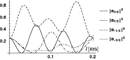
FIG. 6.: Grover algorithm calculated by means of Eq. (95) in the QC scheme, where $\left|s\right>=(1/\sqrt{4})\sum_{m=-3/2}^{3/2}\left|m\right>$ is concentrated mainly into $\left|1/2\right>$ after 0.05 ms for $h_{1}=h_{2}=h_{3}=\hbar\delta_{1}/2g_{N}\mu_{N}=5$ G, $\delta_{2}=\delta_{3}=0$.

It is interesting to note that

$$\lim_{A\rightarrow 0}S_{-3/2,3/2}^{(3)}=\lim_{A\rightarrow 0}S_{-1/2,3/2}^{(2)}=0,$$ (29)

i.e. destructive interference is maximal. However, if

$$A\gg\hbar|\delta_{k}|,\quad k=1,2,3,$$ (30)

destructive interference is negligible. In other words, the most left diagram in Fig. 1 gives the largest contribution to the transition amplitude. This means that this diagram only is responsible for the time evolution of the nuclear spins. So Eq. (30) is the basis condition for finding the Hamiltonian in the generalized rotating frame that describes the time evolution of our nuclear spin system for arbitrary spin lengths $I$ and arbitrary times $t$ (see Sec. V).

IV The standard rotating frame

Before deriving the transformation of the Hamiltonian ${\cal H}$ including many magnetic fields $H_{x,k}(t)$ oscillating at different frequencies $\omega_{k}$ to the generalized rotating frame (see next section), it is instructive to have a look at the transformation of a Hamiltonian ${\cal H}_{\rm s}$ including only a single circularly polarized oscillating magnetic field ${\bf H}_{\bot}(t)=H_{\bot}(\cos\omega t{\bf e}_{x}+\sin\omega t{\bf e}_{y})$ to the standard rotating frame. We start from the Hamiltonian

$${\cal H}_{\rm s} = -g_{N}\mu_{N}[H_{z}I_{z}+H_{\bot}(I_{x}\cos\omega t+I_{y}\sin\omega t)]$$ (31)

$$= -g_{N}\mu_{N}H_{z}I_{z}+g_{N}\mu_{N}\frac{1}{2}H_{\bot}e^{i\omega tI_{z}}I_{x}e^{-i\omega tI_{z}}.$$ (32)

The proof for the second equality can be given as follows: First let us define the function

$$f(\varphi)=e^{i\varphi I_{z}}I_{x}e^{-i\varphi I_{z}}.$$ (33)

The first and second derivative read

$$\frac{df}{d\varphi} = -e^{i\varphi I_{z}}I_{y}e^{-i\varphi I_{z}},$$ (34)

$$\frac{d^{2}f}{d\varphi^{2}} = -f(\varphi).$$ (35)

The solution of the last differential equation is

$$f(\varphi)=A\cos\varphi+B\sin\varphi.$$ (36)

The boundary conditions

$$f(0)=A=I_{x},\quad\left(\frac{df}{d\varphi}\right)_{\varphi=0}=B=-I_{y}$$ (37)

reduce Eq. (36) to

$$f(\varphi)=I_{x}\cos\varphi-I_{y}\sin\varphi,$$ (38)

which proves Eq. (32).

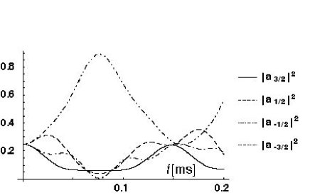
FIG. 7.: Grover algorithm calculated by means of Eq. (95) in the QC scheme, where $\left|s\right>=(1/\sqrt{4})\sum_{m=-3/2}^{3/2}\left|m\right>$ is concentrated mainly into $\left|-3/2\right>$ after 0.05 ms for $h_{1}=h_{2}=h_{3}=\hbar\delta_{3}/2g_{N}\mu_{N}=5$ G, $\delta_{1}=\delta_{3}=0$.

In order to derive the Hamiltonian in the rotating frame, we have to transform the Schrödinger equation

$$i\hbar\frac{\partial\left|\psi\right>}{\partial t}={\cal H}_{\rm s}\left|\psi\right>$$ (39)

with the unitary operation $U$. The left hand side of Eq. (39) transforms into

$$i\hbar\frac{\partial\left|\psi\right>}{\partial t}=i\hbar\left(U^{-1}\frac{\partial\left|\psi_{\rm rot}\right>}{\partial t}+\frac{\partial U^{-1}}{\partial t}\left|\psi_{\rm rot}\right>\right),$$ (40)

and the right hand side of Eq. (39) into

$${\cal H}\left|\psi\right>={\cal H}U^{-1}\left|\psi_{\rm rot}\right>,$$ (41)

where we have defined the state in the rotating frame by $\left|\psi_{\rm rot}\right>=U\left|\psi\right>$. Combining both sides (40) and (41) yields

$$i\hbar\left(U^{-1}\frac{\partial\left|\psi_{\rm rot}\right>}{\partial t}+\frac{\partial U^{-1}}{\partial t}\left|\psi_{\rm rot}\right>\right)={\cal H}U^{-1}\left|\psi_{\rm rot}\right>,$$ (42)

from which we obtain

$$i\hbar\frac{\partial\left|\psi_{\rm rot}\right>}{\partial t}=\left(U{\cal H}U^{-1}-i\hbar U\frac{\partial U^{-1}}{\partial t}\right)\left|\psi_{\rm rot}\right>\equiv{\cal H}_{\rm rot}\left|\psi_{\rm rot}\right>$$ (43)

by multiplying $U$ to Eq. (42) from the left. From Eq. (43) we can immediately read off the Hamiltonian in the rotating frame:

$${\cal H}_{\rm rot}=U{\cal H}U^{\dagger}-i\hbar U\frac{\partial U^{\dagger}}{\partial t}=U{\cal H}U^{\dagger}+i\hbar\frac{\partial U}{\partial t}U^{\dagger}.$$ (44)

If we insert $U(t)=e^{-i\omega tI_{z}}$, we get

$${\cal H}_{\rm rot}=-(g_{N}\mu_{N}H_{z}-\hbar\omega)I_{z}+g_{N}\mu_{N}H_{\bot}I_{x}.$$ (45)

which is completely time-independent. In the next section we will show that under the special condition of quadratic anisotropy we can transform a Hamiltonian with more than one oscillating term into a Hamiltonian that is also completely time-independent.

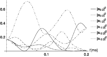
FIG. 8.: Grover algorithm calculated by means of Eq. (95) in the QC scheme, where $\left|s\right>=(1/\sqrt{6})\sum_{m=-5/2}^{5/2}\left|m\right>$ is concentrated mainly into $\left|-1/2\right>$ after 0.05 ms for $h_{1}=h_{2}=h_{3}=h_{4}=h_{5}=\hbar\delta_{3}/2g_{N}\mu_{N}=5$ G, $\delta_{1}=\delta_{2}=\delta_{4}=\delta_{5}=0$.

V The generalized rotating frame

For the case where the Hamiltonian ${\cal H}$ contains many magnetic fields $H_{x,k}(t)$ that oscillate at different frequencies $\omega_{k}$, the transformation to the standard rotating frame cannot be used anymore. In this section we develop a concept that allows us to transform the Hamiltonian ${\cal H}$ into a generalized rotating frame, i.e. ${\cal H}\rightarrow{\cal H}_{\rm grot}$, where ${\cal H}_{\rm grot}$ is completely time-independent. Then the time evolution of the nuclear spins can be calculated non-perturbatively in this generalized rotating frame. In contrast to previous work[26] our method also holds for vanishing detuning energies $\hbar\delta_{k}\rightarrow 0$, which is essential to perform non-perturbative unitary operations. Once the control over $2I$ magnetic fields is established, the scheme proposed here allows for quantum information processing and quantum storage with a single pulse, provided that there is sufficient signal amplification due to the spin ensemble. The only requirements are that the quadrupolar splitting $A$ is much larger than the detuning energies $\delta_{k}$, so that only the most left diagram in Fig. 1 governs the time evolution of the nuclear spins (see Sec. III).

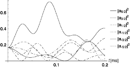
FIG. 9.: Grover algorithm calculated by means of Eq. (95) in the QC scheme, where $\left|s\right>=(1/\sqrt{6})\sum_{m=-5/2}^{5/2}\left|m\right>$ is concentrated mainly into $\left|-3/2\right>$ after 0.05 ms for $h_{1}=h_{2}=h_{3}=h_{4}=h_{5}=\hbar\delta_{4}/2g_{N}\mu_{N}=5$ G, $\delta_{1}=\delta_{2}=\delta_{3}=\delta_{5}=0$.

We first start with the example for two detuning energies $\hbar\delta_{1}$ and $\hbar\delta_{2}$ and give the general derivation for arbitrary spin lengths $I$ afterwards. The corresponding Hamiltonian for three states reads

$${\cal H}^{(2)}=\left[\begin{array}[]{ccc}\varepsilon_{a}&\left<a\left|V\right|b\right>&0\\ \left<b\left|V\right|a\right>&\varepsilon_{b}&\left<b\left|V\right|c\right>\\ 0&\left<c\left|V\right|b\right>&\varepsilon_{c}\end{array}\right],$$ (46)

where $\left|a\right>$, $\left|b\right>$, and $\left|c\right>$ are three consecutive spin states ($a,b,c$ are integers or half-integers with $a=b+1=c+2$, $-I\leq a,b,c\leq I$) with their eigenenergies $\varepsilon_{a},\varepsilon_{b},\varepsilon_{c}$. For example $a=3/2$, $b=1/2$, and $c=-1/2$, which is shown in Fig. 1. If the quadratic anisotropy $A$ is much larger than the detuning energies $\hbar\delta_{k}$, we can neglect all the transition diagrams with blue detuning energies shown in Fig. 1. Applying also the rotating wave approximation leaves us with

$${\cal H}_{\rm app}^{(2)}=\left[\begin{array}[]{ccc}\varepsilon_{a}&h_{1}e^{i\omega_{1}t+i\Phi_{1}}&0\\ h_{1}e^{-i\omega_{1}t-i\Phi_{1}}&\varepsilon_{b}&h_{2}e^{i\omega_{2}t+i\Phi_{2}}\\ 0&h_{2}e^{-i\omega_{2}t-i\Phi_{2}}&\varepsilon_{c}\end{array}\right],$$ (47)

where $h_{1}=H_{1}\left<a\left|I_{x}\right|b\right>$, $h_{2}=H_{2}\left<b\left|I_{x}\right|c\right>$.

The goal is now to find a unitary transformation $U$ that renders our Hamiltonian ${\cal H}_{\rm app}^{(2)}$ time-independent. We know from the previous section that the transformed Hamiltonian has the form

$${\cal H}_{\rm grot}=U{\cal H}_{\rm app}U^{\dagger}-i\hbar U\frac{\partial U^{\dagger}}{\partial t}=U{\cal H}_{\rm app}U^{\dagger}+i\hbar\frac{\partial U}{\partial t}U^{\dagger}.$$ (48)

Instead of inserting $U(t)=e^{-i\omega tI_{z}}$, we make an ansatz with three parameters $\omega_{a}$, $\omega_{b}$, and $\omega_{c}$:

$$U=\left[\begin{array}[]{ccc}e^{-i\omega_{a}t}&0&0\\ 0&e^{-i\omega_{b}t}&0\\ 0&0&e^{-i\omega_{c}t}\end{array}\right].$$ (49)

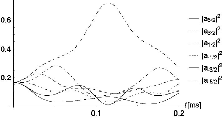
FIG. 10.: Grover algorithm calculated by means of Eq. (95) in the QC scheme, where $\left|s\right>=(1/\sqrt{6})\sum_{m=-5/2}^{5/2}\left|m\right>$ is concentrated mainly into $\left|-5/2\right>$ after 0.05 ms for $h_{1}=h_{2}=h_{3}=h_{4}=h_{5}=\hbar\delta_{5}/2g_{N}\mu_{N}=5$ G, $\delta_{1}=\delta_{2}=\delta_{3}=\delta_{4}=0$.

Evaluation of $U{\cal H}_{\rm app}^{(2)}U^{\dagger}$ yields

$${\cal H}_{\rm grot}^{(2)} = \left[\begin{array}[]{ccc}\varepsilon_{a}&h_{1}e^{i\Omega_{1}t}&0\\ h_{1}e^{-i\Omega_{1}t}&\varepsilon_{b}&h_{2}e^{i\Omega_{2}t}\\ 0&h_{2}e^{-i\Omega_{2}t}&\varepsilon_{c}\end{array}\right]$$ (54)

$$+i\hbar\frac{\partial U}{\partial t}U^{\dagger},$$

with the abbreviations $\Omega_{1}=-\omega_{a}+\omega_{b}+\omega_{1}+\Phi_{1}/t$ and $\Omega_{2}=-\omega_{b}+\omega_{c}+\omega_{2}+\Phi_{2}/t$. Since we want to make the Hamiltonian in Eq. (54) time-independent, we require that

$$\Omega_{1} = -\omega_{a}+\omega_{b}+\omega_{1}+\Phi_{1}/t=0,$$ (55)

$$\Omega_{2} = -\omega_{b}+\omega_{c}+\omega_{2}+\Phi_{2}/t=0.$$ (56)

In this way we get also rid of the Phases $\Phi_{1}$ and $\Phi_{2}$. Solving the Eqs. (55) and (56) gives

$$\omega_{a} = \omega_{1}+\omega_{2}+\omega_{c}+(\Phi_{1}+\Phi_{2})/t,$$ (57)

$$\omega_{b} = \omega_{2}+\omega_{c}+\Phi_{2}/t.$$ (58)

$\omega_{c}$ is a free parameter, which we choose to be $\omega_{c}=-(\omega_{1}+\omega_{2})/2-(\Phi_{1}+\Phi_{2})/2t$. Then Eqs. (57) and (58) simplify to

$$\omega_{a} = (\omega_{1}+\omega_{2})/2+(\Phi_{1}+\Phi_{2})/2t,$$ (59)

$$\omega_{b} = (\omega_{2}-\omega_{1})/2+(\Phi_{2}-\Phi_{1})/2t.$$ (60)

Then the second term in Eq. (48) is

$$i\hbar\frac{\partial U}{\partial t}U^{\dagger}=\left[\begin{array}[]{ccc}\frac{\hbar(\omega_{1}+\omega_{2})}{2}&0&0\\ 0&\frac{\hbar(\omega_{2}-\omega_{1})}{2}&0\\ 0&0&-\frac{\hbar(\omega_{1}+\omega_{2})}{2}\end{array}\right].$$ (61)

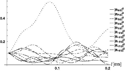
FIG. 11.: Grover algorithm calculated by means of Eq. (95) in the QC scheme, where $\left|s\right>=(1/\sqrt{10})\sum_{m=-9/2}^{9/2}\left|m\right>$ is concentrated mainly into $\left|-1/2\right>$ after 0.05 ms for $h_{1}=h_{2}=h_{3}=h_{4}=h_{5}=h_{6}=h_{7}=h_{8}=h_{9}=\hbar\delta_{5}/2g_{N}\mu_{N}$ $=5$ G, $\delta_{1}=\delta_{2}=\delta_{3}=\delta_{4}=\delta_{6}=\delta_{7}=\delta_{8}=\delta_{9}=0$.

If we insert the external frequencies $\omega_{1}=\varepsilon_{b}/\hbar-\varepsilon_{a}/\hbar-\delta_{1}$ and $\omega_{2}=\varepsilon_{c}/\hbar-\varepsilon_{b}/\hbar+\delta_{1}-\delta_{2}$, we obtain

$${\cal H}_{\rm grot}^{(2)}=\left[\begin{array}[]{ccc}\frac{\varepsilon_{a}+\varepsilon_{c}-\hbar\delta_{2}}{2}&h_{1}&0\\ h_{1}&\frac{\varepsilon_{a}+\varepsilon_{c}+\hbar(2\delta_{1}-\delta_{2})}{2}&h_{2}\\ 0&h_{2}&\frac{\varepsilon_{a}+\varepsilon_{c}+\hbar\delta_{2}}{2}\end{array}\right],$$ (62)

which is equivalent to

$${\cal H}_{\rm grot}^{(2)}=\left[\begin{array}[]{ccc}0&h_{1}&0\\ h_{1}&\hbar\delta_{1}&h_{2}\\ 0&h_{2}&\hbar\delta_{2}\end{array}\right],$$ (63)

where we have subtracted $\frac{\varepsilon_{a}+\varepsilon_{c}-\hbar\delta_{2}}{2}{\rm Id}$. Id is the identity matrix.

Now we give the general derivation for the transformation to the generalized rotating frame for arbitrary spin lengths $I$. From the above derivation, we know that for a spin of arbitrary length $I$ the Hamiltonian in the generalized rotating frame has the form

$${\cal H}_{\rm grot}^{(2I)} = \left[\begin{array}[]{ccccc}\ddots&\ddots&&&\\ \ddots&\varepsilon_{m_{5}}&h_{5}e^{i\Omega_{5}t}&&\\ &h_{5}e^{-i\Omega_{5}t}&\varepsilon_{m_{6}}&h_{6}e^{i\Omega_{6}t}&\\ &&h_{6}e^{-i\Omega_{6}t}&\varepsilon_{m_{7}}&\ddots\\ &&&\ddots&\ddots\end{array}\right]$$ (70)

$$+i\hbar\frac{\partial U}{\partial t}U^{\dagger},$$

which has non-zero entries only in the diagonal and first off-diagonal lines. $\left|m_{0}\right>=\left|2I\right>,\left|m_{1}\right>=\left|2I-1\right>,\ldots,\left|m_{2I}\right>=\left|-2I\right>$ are the eigenstates of the Hamiltonian shown in Eq. (1) with eigenenergies $\varepsilon_{m_{0}},\varepsilon_{m_{1}},\ldots,\varepsilon_{m_{2I}}$. The unitary transformation reads

$$U=\left[\begin{array}[]{ccccc}\ddots&&&&\\ &e^{-i\omega_{m_{5}}t}&&&\\ &&e^{-i\omega_{m_{6}}t}&&\\ &&&e^{-i\omega_{m_{7}}t}&\\ &&&&\ddots\end{array}\right],$$ (71)

with only diagonal elements that are non-zero.

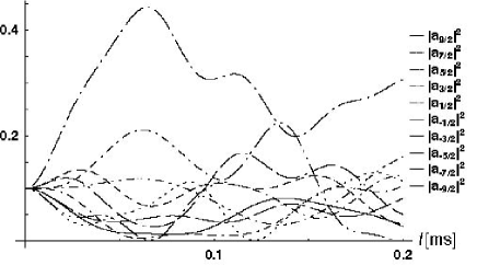
FIG. 12.: Grover algorithm calculated by means of Eq. (95) in the QC scheme, where $\left|s\right>=(1/\sqrt{10})\sum_{m=-9/2}^{9/2}\left|m\right>$ is concentrated mainly into $\left|-3/2\right>$ after 0.05 ms for $h_{1}=h_{2}=h_{3}=h_{4}=h_{5}=h_{6}=h_{7}=h_{8}=h_{9}=\hbar\delta_{6}/2g_{N}\mu_{N}$ $=5$ G, $\delta_{1}=\delta_{2}=\delta_{3}=\delta_{4}=\delta_{5}=\delta_{7}=\delta_{8}=\delta_{9}=0$.

For ${\cal H}_{\rm grot}^{(2I)}$ to be time-independent we have to solve $2I$ linear equations of the form

$$\Omega_{1} = -\omega_{m_{0}}+\omega_{m_{1}}+\omega_{1}+\Phi_{1}/t=0,$$ (72)

$$\Omega_{2} = -\omega_{m_{1}}+\omega_{m_{2}}+\omega_{2}+\Phi_{2}/t=0,$$ (73)

$$\vdots$$ (74)

$$\Omega_{5} = -\omega_{m_{5}}+\omega_{m_{6}}+\omega_{5}+\Phi_{5}/t=0,$$ (75)

$$\Omega_{6} = -\omega_{m_{6}}+\omega_{m_{7}}+\omega_{6}+\Phi_{6}/t=0,$$ (76)

$$\vdots$$ (77)

$$\Omega_{2I-1} = -\omega_{m_{2I-2}}+\omega_{m_{2I-1}}+\omega_{2I-1}+\Phi_{2I-1}/t=0,$$ (78)

$$\Omega_{2I} = -\omega_{m_{2I-1}}+\omega_{m_{2I}}+\omega_{2I}+\Phi_{2I}/t=0,$$ (79)

Summing over all linear equations (72) to (79) leads to

$$\omega_{m_{0}}=\omega_{m_{2I}}+\sum\limits_{k=1}^{2I}(\omega_{k}+\Phi_{k}/t),$$ (80)

where $\omega_{m_{2I}}$ can be chosen arbitarily. Inserting this result back into the linear equations (72) to (79) gives

$$\omega_{m_{1}} = \omega_{m_{2I}}+\sum\limits_{k=2}^{2I}(\omega_{k}+\Phi_{k}/t),$$ (81)

$$\omega_{m_{2}} = \omega_{m_{2I}}+\sum\limits_{k=3}^{2I}(\omega_{k}+\Phi_{k}/t),$$ (82)

$$\vdots$$ (83)

$$\omega_{m_{5}} = \omega_{m_{2I}}+\sum\limits_{k=6}^{2I}(\omega_{k}+\Phi_{k}/t),$$ (84)

$$\omega_{m_{6}} = \omega_{m_{2I}}+\sum\limits_{k=7}^{2I}(\omega_{k}+\Phi_{k}/t),$$ (85)

$$\vdots$$ (86)

$$\omega_{m_{2I-1}} = \omega_{m_{2I}}+\sum\limits_{k=2I}^{2I}(\omega_{k}+\Phi_{k}/t).$$ (87)

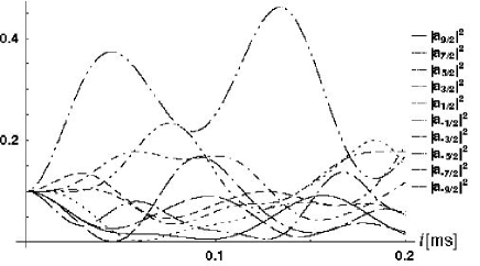
FIG. 13.: Grover algorithm calculated by means of Eq. (95) in the QC scheme, where $\left|s\right>=(1/\sqrt{10})\sum_{m=-9/2}^{9/2}\left|m\right>$ is concentrated mainly into $\left|-5/2\right>$ after 0.05 ms for $h_{1}=h_{2}=h_{3}=h_{4}=h_{5}=h_{6}=h_{7}=h_{8}=h_{9}=\hbar\delta_{7}/2g_{N}\mu_{N}=5$ G, $\delta_{1}=\delta_{2}=\delta_{3}=\delta_{4}=\delta_{5}=\delta_{6}=\delta_{8}=\delta_{9}=0$.

Then the second term in Eq. (70) $i\hbar\frac{\partial U}{\partial t}U^{\dagger}$ has the diagonal elements $\hbar(\omega_{m_{2I}}+\sum_{k=1}^{2I}\omega_{k}),\hbar(\omega_{m_{2I}}+\sum_{k=2}^{2I}\omega_{k}),\ldots,\hbar(\omega_{m_{2I}}+\sum_{k=2I}^{2I}\omega_{k}),\hbar\omega_{m_{2I}}.$ All the off-diagonal elements of $i\hbar\frac{\partial U}{\partial t}U^{\dagger}$ are zero. The external frequencies are

$$\omega_{1} = \varepsilon_{m_{1}}/\hbar-\varepsilon_{m_{0}}/\hbar-\delta_{1}$$ (88)

$$\omega_{2} = \varepsilon_{m_{2}}/\hbar-\varepsilon_{m_{1}}/\hbar-\delta_{2}+\delta_{1}$$ (89)

$$\vdots$$ (90)

$$\omega_{5} = \varepsilon_{m_{5}}/\hbar-\varepsilon_{m_{4}}/\hbar-\delta_{5}+\delta_{4}$$ (91)

$$\omega_{6} = \varepsilon_{m_{6}}/\hbar-\varepsilon_{m_{5}}/\hbar-\delta_{6}+\delta_{5}$$ (92)

$$\vdots$$ (93)

$$\omega_{2I} = \varepsilon_{m_{2I}}/\hbar-\varepsilon_{m_{2I-1}}/\hbar-\delta_{2I}+\delta_{2I-1}$$ (94)

After setting $\omega_{m_{2I}}=0$, we then obtain for the diagonal elements of $i\hbar\frac{\partial U}{\partial t}U^{\dagger}$ the following results: $(-\varepsilon_{m_{0}}+\varepsilon_{m_{2I}}-\hbar\delta_{2I}),(-\varepsilon_{m_{1}}+\varepsilon_{m_{2I}}+\hbar\delta_{1}-\hbar\delta_{2I}),(-\varepsilon_{m_{2}}+\varepsilon_{m_{2I}}+\hbar\delta_{2}-\hbar\delta_{2I}),\ldots,(-\varepsilon_{m_{2I-1}}+\varepsilon_{m_{2I}}+\hbar\delta_{2I-1}-\hbar\delta_{2I}),0.$ Finally, subtracting $(\varepsilon_{m_{2I}}-\hbar\delta_{2I})$Id from ${\cal H}_{\rm grot}^{(2I)}$ in Eq. (70) yields the time-independent Hamiltonian

$${\cal H}_{\rm grot}^{(2I)}=\left[\begin{array}[]{ccccc}0&h_{1}&0&\cdots&0\\ h_{1}&\hbar\delta_{1}&h_{2}&\ddots&\vdots\\ 0&h_{2}&\hbar\delta_{2}&\ddots&0\\ \vdots&\ddots&\ddots&\ddots&h_{2I}\\ 0&\cdots&0&h_{2I}&\hbar\delta_{2I}\end{array}\right].$$ (95)

This Hamiltonian allows us to evaluate the time evolution of the nuclear spin system for arbitrary spin lengths $I$ and arbitrary times $t$ non-perturbatively. Note that the Hamiltonian in Eq. (95) remains valid even in the limit $\delta_{k}\rightarrow 0$, where the perturbation expansions for multiphoton (more than 1) transition amplitudes, such as in Eqs. (26) and (27), break down. However, we must require that $|g_{N}\mu_{N}H_{k}|\ll|A|$, which means that the larger $|A|$, the faster the quantum information processing (see Ref. [17]). The time evolution of the state $\left|\psi(t)\right>$ reads

$$\left|\psi(t)\right>=U^{\dagger}(t)e^{-i{\cal H}_{\rm grot}^{(2I)}t/\hbar}\left|\psi(t=0)\right>.$$ (96)

Propagators of the form $U^{\dagger}(t)e^{-i{\cal H}_{\rm grot}^{(2I)}t/\hbar}$ have $2I$ phases $\Phi_{k}$ and $2I$ detunings $\hbar\delta_{k}$, which determine the $2I$ phases and the $2I$ moduli of $a_{m}$. We subtracted two degrees of freedom: the global phase and the normalization condition, respectively. In this way we can produce a state $\left|\psi(t)\right>$ with arbitrary amplitudes $a_{m}$.

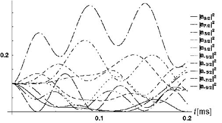
FIG. 14.: Grover algorithm calculated by means of Eq. (95) in the QC scheme, where $\left|s\right>=(1/\sqrt{10})\sum_{m=-9/2}^{9/2}\left|m\right>$ is concentrated mainly into $\left|-7/2\right>$ after 0.05 ms for $h_{1}=h_{2}=h_{3}=h_{4}=h_{5}=h_{6}=h_{7}=h_{8}=h_{9}=\hbar\delta_{8}/2g_{N}\mu_{N}=5$ G, $\delta_{1}=\delta_{2}=\delta_{3}=\delta_{4}=\delta_{5}=\delta_{6}=\delta_{7}=\delta_{9}=0$.

VI The Grover algorithm

Now we make use of the non-perturbative calculation method shown in the previous section to compute the Grover algorithm. We start from a configuration where mainly the ground state $\left|3/2\right>$ is populated, see Fig. 1. This can be achieved by the Overhauser effect[29]. Then we produce an equal superposition of the nuclear spin states $\left|s\right>=(1/\sqrt{n})\sum_{m}\left|m\right>$, which represents the initial state of the Grover algorithm. $n$ is the number of basis states involved in the search. For example we can prepare the state $\left|s\right>=(1/\sqrt{3})\sum_{m=-1/2}^{3/2}\left|m\right>$ with the parameters $H_{1}=H_{2}=1$ G, $H_{3}=0$, $\delta_{1}=6083$ s^-1, and $\delta_{2}=0$, which is shown in Fig. 2. In Fig. 3 we calculated the time evolution of $\left|s\right>$ exactly by solving the Schrödinger equation numerically. This calculation reveals small oscillations that are mainly due to the five neglected diagrams in Fig. 1.

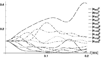
FIG. 15.: Grover algorithm calculated by means of Eq. (95) in the QC scheme, where $\left|s\right>=(1/\sqrt{10})\sum_{m=-9/2}^{9/2}\left|m\right>$ is concentrated mainly into $\left|-9/2\right>$ after 0.2 ms for $h_{1}=h_{2}=h_{3}=h_{4}=h_{5}=h_{6}=h_{7}=h_{8}=h_{9}=\hbar\delta_{9}/2g_{N}\mu_{N}=5$ G, $\delta_{1}=\delta_{2}=\delta_{3}=\delta_{4}=\delta_{5}=\delta_{6}=\delta_{7}=\delta_{8}=0$.

Next, we choose one basis state $\left|M\right>$ to be the one that we are looking for. Since we encode the information into the eigenenergies $\delta_{I-m}$ of the eigenstates $\left|m\right>$ in the generalized rotating frame, we can choose $\delta_{I-m}=0$ for all $m$, except for $M$, i.e. $\delta_{I-M}\neq 0$. In order to find $\left|M\right>$, we make it degenerate with the state $\left|s\right>$ in the generalized rotating frame. So $\delta_{I-M}=\left<s\left|{\cal H}_{\rm grot}^{(2I)}\right|s\right>\neq 0$. As we want to obtain the highest speed for the quantum information processing, the best choice for the Zeeman fields is to make them all equal, i.e. $h_{1}=h_{2}=\ldots=h_{2I}=:h$. The degeneracy condition now leads to

$$\left<s\left|{\cal H}_{\rm grot}^{(2I)}\right|s\right>=\frac{1}{n}(2n-2)h+\frac{1}{n}\sum_{k=1}^{2I}\hbar\delta_{k}\stackrel{{\scriptstyle!}}{{=}}\hbar\delta_{I-M},$$ (97)

from which we obtain directly

$$h=\frac{\hbar\delta_{I-M}}{2}.$$ (98)

We continue the above example, where we have prepared the state $\left|s\right>=(1/\sqrt{3})\sum_{m=-1/2}^{3/2}\left|m\right>$. After making $\left|s\right>$ degenerate with $\left|-1/2\right>$ in the generalized rotating frame, i.e. $\left<s\left|{\cal H}_{\rm grot}^{(3)}\right|s\right>=\hbar\delta_{2}$, the amplitude concentrates mainly into the state $\left|-1/2\right>$ after 0.2 ms. In contrast to Refs. [27, 28], the Hamiltonian in Eq. (95) has only nearest-neighbor couplings, which results in a decreasing amplification of $\left|M\right>$ with increasing $I$ or $|M|$. However, even for the largest nuclear spin $I=9/2$, we find that the resolution for identifying $\left|M\right>$ is still sufficient, i.e. greater than 10% (see below). Again, we have also calculated this time evolution exactly by solving the Schrödinger equation numerically, which is shown in Fig. 5. The small oscillations due to the five neglected diagrams in Fig. 1 are now almost invisible. Thus the larger the quadrupolar splitting $A$, the better the agreement between our non-perturbative method and exact numerics.

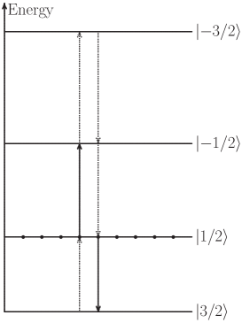
FIG. 16.: In this example only the state $\left|1/2\right>$ is fully populated after performing the Grover algorithm. For the readout of this state, we have to irradiate the nuclear spin system with magnetic fields that oscillate at frequencies that match exactly the level separations.

We have also calculated the Grover sequence for spin lengths up to $I=9/2$. In all the cases for all spin lengths up to $I=9/2$ and for all the searchable states $-I\leq M\leq I$ the Grover sequence leads to an amplification of the amplitude of $\left|M\right>$ between about 10% and 100%. In Figs. 6 and 7 the spin has length $I=3/2$ and the searched state is $\left|M=1/2\right>$ and $\left|M=-3/2\right>$, respectively. When we increase the spin length $I$, the most interesting elements for applications in semiconductors are ²⁷Al, ⁵⁵Mn, and ⁶⁷Zn with nuclear spin $I=5/2$, and ⁷³Ge and ¹¹³In with nuclear spin $I=9/2$. Therefore we have computed the Grover sequence for $I=5/2$ and $M=-1/2,-3/2,-5/2$, which can be seen in Figs. 8, 9, 10, respectively, and also for $I=9/2$ and $M=-1/2,-3/2,-5/2,-7/2,-9/2$, which is shown in Figs. 11, 12, 13, 14, 15, respectively. Because of the symmetry of the Hamiltonian in Eq. (95) along the diagonal, the two computations for $\pm M$ look always the same. Hence, we have shown the Grover sequence only for half of the states $-I\leq M<0$.

VII Readout of the result

After we have performed the Grover quantum search algorithm, we wish to extract the final state that we have been searching for. This can be achieved by using conventional pulsed NMR, where no coherence is required. Fig. 16 demonstrates an example where only the state $\left|1/2\right>$ is completely populated. If we irradiate the sample with magnetic fields $H_{x,k}(t)$ with zero detuning energies $\delta_{k}=0$ $\forall k$, where the external frequencies are tuned in such a way that they match the energy level spaces, i.e. $\omega_{I-m}=\varepsilon_{m+1}-\varepsilon_{m}$, then we induce only emission from $\left|1/2\right>$ to $\left|3/2\right>$ and absorption from $\left|1/2\right>$ to $\left|-1/2\right>$. The emission and absorption spectrum shown in Fig. 17 identifies unambigously the state $\left|1/2\right>$. In this way we can read out any information stored in the nuclear spin system.

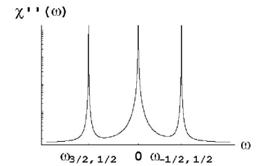
FIG. 17.: The absorption and emission spectrum identifies then unambigously the state $\left|1/2\right>$ for the example shown in Fig. 16.

VIII Conclusion

In our theoretical proposal we have shown that the Grover algorithm can be performed in the nuclear spin system of semiconductors. The main requirement for the Grover algorithm to work is the anisotropy in the spin system, which is provided by the quadrupolar splitting. The reason is that the quadrupolar splitting makes the energy levels non-equidistant, which renders the nuclear spin states distinguishable. Only then we can find an effective Hamiltonian of the form shown in Eq. (95) that describes the coherent time evolution of the nuclear spin ensemble for arbitrary spin lengths and times. It turned out that the larger the quadrupolar splitting, the better the agreement between our non-perturbative method using the effective Hamiltonian and exact numerical calculations. So the larger the symmetry breaking of the energy spacings, the better the control over the coherent time evolution of the nuclear spin system.

The first test for the experimental feasibility of our proposal would be the implementation of multiphoton Rabi oscillations, as proposed in Ref. [17]. This can be achieved by applying only one oscillating magnetic field. Fig. 18 shows a 2-photon Rabi oscillation between the states $\left|3/2\right>$ and $\left|-1/2\right>$ for a nuclear spin $I=3/2$. In general, multiphoton Rabi oscillations can be thought of as nutation of the large spin between the spin states $\left|m\right>$.

Once our scheme works experimentally, it would be interesting to apply a longitudinal magnetic field that has a large gradient. In this case the semiconductor sample could be divided into several regions, each of which could be addressed separately by different transverse magnetic fields. In this way one could perform parallel quantum information processes in each of the regions. Instead of using a large gradient field, it would also be possible to vary the g-factor in the sample, as was shown in the experiment of Ref. [30] for the electron spin in Al_xGa_1-xAs, where the variation of the concentration of Al $x$ leads to a variation of the electron g-factor.

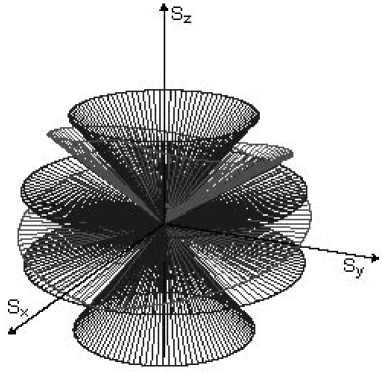
FIG. 18.: 2-photon Rabi oscillation between the states $\left|3/2\right>$ and $\left|-1/2\right>$ for a nuclear spin $I=3/2$.

IX Acknowledgement

We thank M. E. Flatté for useful comments. We acknowledge the Swiss NSF, NCCR Nanoscience, and the US NSF and DARPA for financial support.

REFERENCES

[1] J. M. Kikkawa, D. D. Awschalom, Phys. Rev. Lett. 80, 4313 (1998).
[2] J. M. Kikkawa, D. D. Awschalom, Nature 397, 139 (1999).
[3] G. A. Prinz, Science 282, 1660 (1998).
[4]
S. A. Wolf, D. D. Awschalom, R. A. Buhrman, J. M. Daughton, S. von Molnar,
M. L. Roukes, A. Y. Chtchelkanova, D. M. Treger, Science 294, 1488 (2001).
[5] D. D. Awschalom, D. Loss, N. Samarth, Semiconductor Spintronics and Quantum Computation
(Springer, 2002).
[6] M. Ziese, M. J. Thornton,
Spin Electronics (Lecture Notes in Physics, 569) (Springer, 2001).
[7] A. Chtchelkanova, S. A. Wolf, Y. Idzerda, Magnetic Interactions and Spin Transport
(Plenum Pub Corp, 2003).
[8] D. Loss, D. P. DiVincenzo, Phys. Rev. A 57, 120 (1998).
[9] M. A. Nielsen, I. L. Chuang, Quantum Computation and Quantum Information
(Cambridge U. Press, New York, 2000).
[10] D. Bouwmeester, A. Ekert, A. Zeilinger,
The Physics of Quantum Information (Springer, 2000).
[11] S. Braunstein, H.-K. Lo, Scalable Quantum Computers: Paving the Way
to Realization (Wiley, 2001).
[12] C. Williams, S. Clearwater, Explorations in Quantum Computing
(Telos, 1998).
[13] G. Berman, G. Doolen, R. Mainieri, V. Tsifrinovitch,
Introduction to Quantum Computers (World Scientific, 1998).
[14] H.-K. Lo, S. Popescu, T. Spiller,
Introduction to Quantum Computation and Information (World Scientific, 1998).
[15] A. Yu Kitaev, A. H. Shen, M. N. Vyalyi, Classical and Quantum Computation
(American Mathematical Society, 2002).
[16] G. Johnson, A Shortcut Through Time: The Path to a Quantum Computer (Knopf, 2003).
[17] M. N. Leuenberger, D. Loss, M. Poggio, D. D. Awschalom,
Phys. Rev. Lett. 89, 207601 (2002).
[18] M. N. Leuenberger, D. Loss, M. E. Flatté, D. D. Awschalom,
cond-mat/0302279.
[19] J. M. Kikkawa, D. D. Awschalom, Science 287,
473 (2000).
[20] G. Salis, D. T. Fuchs, J. M. Kikkawa, D. D. Awschalom, Y. Ohno, H. Ohno,
Phys. Rev. Lett. 86, 2677 (2001);
G. Salis, D. D. Awschalom, Y. Ohno, H. Ohno,
Phys. Rev. B 64, 195304 (2001).
[21] A. Abragam, The Principles of Nuclear Magnetism
(Clarendon, 1961).
[22] J. H. Smet, R. A. Deutschmann, F. Ertl, W. Wegscheider, G. Abstreiter,
K. von Klitzing, Nature 415, 281 (2002).
[23] R. K. Kawakami, Y. Kato, M. Hanson, I. Malajovich, J. M. Stephens,
E. Johnston-Halperin, G. Salis, A. C. Gossard, D. D. Awschalom, Science 294, 131 (2001).
[24] L. K. Grover, Phys. Rev. Lett. 79, 4709 (1997).
[25] J. Ahn, T. C. Weinacht, P. H. Bucksbaum, Science 287, 463 (2000).
[26] M. N. Leuenberger, D. Loss, Nature 410,
789 (2001).
[27] E. Farhi, S. Gutmann, Phys. Rev. A 57, 2403 (1998).
[28] L. K. Grover, A. M. Sengupta, Phys. Rev. A 65, 032319 (2002).
[29] S. E. Barrett, R. Tycko, L. N. Pfeiffer, K. W. West, Phys. Rev. Lett. 72,
1368 (1994); J. A. Marohn, P. J. Carson, J. Y. Hwang, M. A. Miller, D. N. Shykind, D. P. Weitekamp, Phys. Rev. Lett. 75, 1364
(1995).
[30] G. Salis, Y. Kato, K. Ensslin, D. C. Driscoll, A. C. Gossard, D. D. Awschalom,
Nature 414, 619 (2001).