Probe-configuration dependent dephasing in a mesoscopic interferometer

Abstract

Dephasing in a ballistic four-terminal Aharonov-Bohm geometry due to charge and voltage fluctuations is investigated. Treating two terminals as voltage probes, we find a strong dependence of the dephasing rate on the probe configuration in agreement with a recent experiment by Kobayashi et al. (J. Phys. Soc. Jpn. 71, 2094 (2002)). Voltage fluctuations in the measurement circuit are shown to be the source of the configuration dependence.

Recently, Kobayashi et al. kobayashi measured the reduction of the Aharonov-Bohm (AB) effect ab in a ballistic four-terminal ring due to decoherence and thermal averaging. Not only was the visibility of the AB-oscillations found to be much larger in the non-local configuration (see Fig.(1)), but also decoherence was observed to be considerably weaker than in the local configuration (see Fig.(1)). That the external measurement circuit can strongly influence the physical properties of a mesoscopic conductor has been shown for a variety of problems ranging from dephasing in disordered conductors aak to Coulomb blockade devoret or the higher moments of the noise in a tunnel junction beenakker . However, to our knowledge the experiment of Kobayashi et al. kobayashi provides the first experimental evidence of such a striking dependence of the coherence properties of open mesoscopic conductors on the measurement configuration. The purpose of this letter is to provide a theoretical explanation of this phenomenon.

In the experiment of Ref. kobayashi , the decoherence rate was extracted from a measurement of the four-terminal resistance $R_{\alpha\beta,\gamma\delta}$. The two contacts $\alpha,\beta$ are voltage biased and monitored by an ampmeter while the two contacts $\gamma,\delta$ are connected to a voltmeter. In mesoscopic transport, the four-probe character of resistance measurements markus_four_term becomes apparent if the probes are within a coherence volume of the sample webb . A resistance measurement is termed local if the voltage probes are along the current path and is termed non-local if the voltage probes are far from the current path. For the conductor shown in Fig. (1), $R_{14,23}$ is a local resistance, whereas $R_{12,34}$ is an example of a non-local resistance. We emphasize that the sample is the same, independent of the resistance measured: what changes is how the sample is connected to the current source and to the voltmeter.

AB oscillations are the result of quantum interference from electrons travelling through the two arms of the ring. In ballistic mesoscopic rings these oscillations can be larger than 50% of the total current amplitude kobayashi ; kayser ; ji , and their decay is a measure of decoherence in the system (once thermal averaging is taken into account). Experimental investigations casse ; hansen found a linear temperature dependence of the dephasing rate hansen . A theoretical explanation, starting from fluctuating electrostatic potentials in the ring, is given in Ref. seelig . Similar results for the temperature dependence of the dephasing rate, both experimental bird ; clarke and theoretical takane , have been obtained previously for chaotic quantum dots. Here, we are concerned with another feature of the dephasing rate, namely its probe configuration dependence kobayashi .

Figure 1: Ballistic four-terminal ring: An internal potential $U_{i}(t)$ and a charge $+Q_{i}(t)$ belong to each arm of the ring ($i=A,B$). Each arm is coupled to a side-gate via a capacitance $C_{i}$. The local and non-local voltage-probe configurations are indicated.

First, we illustrate our approach for a (reflectionless) electronic Mach-Zehnder interferometer (MZI) seelig . In a second step, we consider interferometers with backscattering at the intersections. In both cases, the arms of the ring are treated as perfect one-channel leads that can be charged up relative to nearby side-gates via the capacitances $C_{A}$ and $C_{B}$. The setup is sketched in Fig. (1). For the MZI, the intersections are described as reflectionless beam splitters (see inset in Fig. (2)) with a scattering matrix

$${\bf S}_{B}=\left(\begin{array}[]{ll}0&{\bf s}\\ {\bf s}&0\end{array}\right),\,\,\,\,{\bf s}=\left(\begin{array}[]{cc}\sqrt{{\cal T}}&i\sqrt{1-{\cal T}}\\ i\sqrt{1-{\cal T}}&\sqrt{{\cal T}}\end{array}\right).$$ (1)

Here, $\sqrt{{\cal T}}$ is the amplitude for going straight through the intersection and $i\sqrt{1-{\cal T}}$ the amplitude for being deflected. Due to the absence of backscattering, the MZI does not exhibit closed electronic trajectories.

Electron-electron interactions give rise to fluctuations of the internal potentials $U_{i}(t)$ ($i=A,B$). In the presence of interactions, the dimensionless conductance $G_{13}$ relating current at contact 1 to a voltage applied to contact 3 is seelig

$$G_{13}=-\langle T_{13}\rangle=-2{\cal T}(1-{\cal T})\left[1+{\rm e}^{-\tau\Gamma_{\phi}}\cos\left(2\pi\Phi\right)\right].$$ (2)

Here, $T_{13}$ is the transmission probability, $\tau=L/v_{F}$ is the traversal time, $\Phi$ is the magnetic flux through the ring (in units of the flux quantum) and we have taken equal arm lengths in the ring, $L_{A}=L_{B}=L$. The angular brackets denote an average over the potential fluctuations in the ring thermal . In the limit of classical Nyquist noise, the decoherence rate

$$\Gamma_{\phi}=\frac{e^{2}}{2\hbar^{2}}\Sigma_{UU}(0)$$ (3)

is then proportional to the spectral function $\Sigma_{UU}(0)$ of the potential difference $U(t)=U_{A}(t)-U_{B}(t)$ in the zero-frequency limit. If all four contacts are connected to a zero-impedance external circuit kept at constant voltage, the rate $\Gamma_{\phi}$ of dephasing due to (small energy transfer) electron-electron scattering is

$$\gamma^{0}_{\phi}=\frac{2kTe^{2}}{\hbar^{2}}\left(\frac{C_{\mu}}{C}\right)^{2}R_{q}.$$ (4)

Here, $T$ is the temperature, $R_{q}=h/(4e^{2})$ is the charge relaxation resistance and the electrochemical capacitance $C^{-1}_{\mu}=C^{-1}+(e^{2}D)^{-1}$ is the series combination of the geometrical capacitance and the density of states ap1 . We assumed $C_{A}=C_{B}=C$.

In the experiment of Ref. kobayashi , two probes are connected to a voltmeter which ideally has infinite impedance. The voltage at a lead connected to the voltmeter fluctuates to maintain zero net current. These voltage fluctuations give rise to fluctuations of the internal potentials which in turn leads to additional dephasing. For the interferometer shown in Fig. (1), this new contribution to the dephasing rate turns out to depend strongly on the probe configuration. For the dephasing rates in the local ($\it l$) and non-local ($\it nl$) configuration we obtain respectively,

$$\Gamma^{l}_{\phi}=\gamma^{0}_{\phi}+\gamma^{l}_{\phi}, \,\,\,\gamma^{l}_{\phi}=\gamma^{0}_{\phi}\,\frac{(2{\cal T}-1)^{2}}{2{\cal T}(1-{\cal T})+T_{0}},$$ (5a)

$$\Gamma^{nl}_{\phi}=\gamma^{0}_{\phi}+\gamma^{nl}_{\phi}, \,\,\,\gamma^{nl}_{\phi}=\gamma^{0}_{\phi}\,\frac{(2{\cal T}-1)^{2}}{1+2T_{0}}.$$ (5b)

Here, $\gamma^{l}_{\phi}$ and $\gamma^{nl}_{\phi}$ are the probe-configuration specific contributions. The experiment of Ref. kobayashi shows transmission between neighboring contacts to be significant. For better comparison, we therefore included a finite incoherent transmission $T_{0}=T_{12}=T_{21}=T_{34}=T_{43}$ (see Fig. (2)).

The results for the dephasing rates are strongly dependent on the symmetry of the interferometer. In the symmetric case (${\cal T}=1/2$) the contribution to the dephasing rate due to voltage fluctuations vanishes for both measurement configurations.

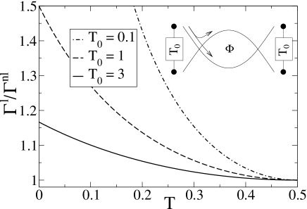
Figure 2: The ratio of the local to the non-local decoherence rate is shown as a function of the transmission ${\cal T}$ at the beam splitters for different values of the incoherent parallel resistance $1/T_{0}$. All curves are symmetric with respect to ${\cal T}=1/2$. In the inset, the two possible electron paths at the beam-splitter and the resistance $1/T_{0}$ (in units of $h/e^{2}$) are indicated.

Away from the symmetry point, ${\cal T}=1/2$, the local and non-local decoherence rate differ strongly pilgram . A local decoherence rate several times larger than the non-local one can easily be obtained for small enough $T_{0}$. The ratio of the decoherence rates for the two probe configurations is shown in Fig. (2) as a function of the transmission probability ${\cal T}$.

To derive the results presented in Eqs. (5a) and (5b), we need to know the spectral function $\Sigma_{UU}(0)$ for the two different probe configurations. To start with, we want to express the Fourier transform $\Delta U(\omega)=\Delta U_{A}(\omega)-\Delta U_{B}(\omega)$ of the fluctuations of the internal potential operator through the operators for the bare charge $\Delta Q^{b}_{i}(\omega)$ ($i=A,B$) and current $\Delta I^{b}_{\alpha}(\omega)$ ($\alpha=1,\ldots,4$) fluctuations in the sample. For these quantities it is known how to calculate the spectral functions. The notation $\Delta{\cal O}={\cal O}-\langle{\cal O}\rangle$ denotes deviations of an operator $\cal O$ from its expectation value. There are two independent equations relating charge and potential fluctuations, namely,

$$\Delta Q_{i}=C\Delta U_{i}=\Delta Q^{b}_{i}-e^{2}D\Delta U_{i}+e^{2}\sum_{\alpha}D^{(i)}_{\alpha}\Delta V_{\alpha}.$$ (6)

Here, $\Delta Q^{b}_{i}(\omega)$ are the charge fluctuations at constant voltage and internal potential and $\Delta V_{\alpha}$ are the voltage fluctuations at contact $\alpha$. The response to a change in the applied voltage at contact $\alpha$ is determined by the average injectivity $D^{(i)}_{\alpha}(\omega)=\langle D^{(i)}_{\alpha\alpha}(\omega)\rangle=\partial\langle Q_{i}\rangle/e^{2}\partial V_{\alpha}$. The term with the negative sign in Eq. (6) is the screening charge induced in response to a change in the internal potential. In the Thomas-Fermi approximation, the response function is the density $D(\omega)=-\partial\langle Q_{i}\rangle/e^{2}\partial U_{i}$. For zero frequency, we find $D=\sum_{\alpha}D^{(i)}_{\alpha}=2L/hv_{F}$ as a consequence of gauge invariance. The injectivities are the diagonal elements of the local density of states (DOS) matrix pedersen ; martin which is related to the scattering matrix $S_{\alpha\beta}$ of the system. In the zero-frequency limit

$$D^{(i)}_{\alpha\beta}(E)=-\frac{1}{2\pi i}\sum_{\gamma}S^{\dagger}_{\gamma\alpha}(E)\frac{dS_{\gamma\beta}(E)}{edU_{i}}$$ (7)

with $i=A,B$ and $\alpha,\beta,\gamma=1,\ldots,4$. The scattering matrix for the electronic interferometer can be derived using Eq. (1) (see also Ref. seelig ).

The voltage fluctuations entering Eq. (6) are related to the current fluctuations $\Delta I_{\alpha}$ through markus_noise

$$\Delta I_{\alpha}=\Delta I^{b}_{\alpha}+\sum_{\beta}G_{\alpha\beta}\Delta V_{\beta}.$$ (8)

In this Langevin-like equation, $\Delta I^{b}_{\alpha}$ are the bare current fluctuations and $G_{\alpha\beta}=G_{0}(M_{\alpha}\delta_{\alpha\beta}-\langle T_{\alpha\beta}\rangle)$ are elements of the conductance matrix ($\alpha,\beta=1,\ldots,4$). For the MZI we have $M_{\alpha}=1+T_{0}$ where $T_{0}$ is the incoherent transmission between neighboring external leads at the same intersection. The probabilities for coherent transmission are $T_{\alpha\beta}=|S_{\alpha\beta}|^{2}$. The central new ingredient in this paper are the boundary conditions imposed on the voltage fluctuations $\Delta V_{\alpha}$ and the fluctuations of the total currents $\Delta I_{\alpha}$ by the external measurement circuit. These boundary conditions depend on the measurement configuration. In the local configuration (see Fig. (1)) we choose contacts $1$ and $4$ as the current probes (they exhibit no voltage fluctuations: $\Delta V_{1}=\Delta V_{4}=0$) while contacts $2$ and $3$ are the voltage probes (no current fluctuations: $\Delta I_{2}=\Delta I_{3}=0$). In the non-local configuration, on the other hand, the voltage probes are contacts 3 and 4 (cf. Fig. (1)) and thus $\Delta V_{1}=\Delta V_{2}=0$ and $\Delta I_{3}=\Delta I_{4}=0$. Eq. (8), together with the boundary conditions for voltages and currents, can now be used to eliminate the voltage fluctuations in Eq. (6) in favor of the fluctuations of the bare currents. The potential fluctuations $\Delta U$ can then be expressed through the fluctuations of the bare currents $\Delta I^{b}_{\alpha}$ and charges $\Delta Q^{b}_{i}$. The result for $\Delta U$ will be different for the local and non-local configuration as a consequence of the different boundary conditions.

The spectral function of the potential fluctuations is defined through the relation $2\pi\delta(\omega+\omega^{\prime})\Sigma_{UU}(\omega)=\langle\Delta U(\omega)\Delta U(\omega^{\prime})+\Delta U(\omega^{\prime})\Delta U(\omega)\rangle/2$. Since we now know how to express the potential fluctuations for the local and non-local case through the fluctuations of the bare currents and charges, we can also express the spectral function $\Sigma_{UU}(\omega)$, through the correlators of the bare charge $\Sigma_{Q^{b}_{i}Q^{b}_{k}}(\omega)$ ($i,k=A,B$), the current correlators $\Sigma_{I^{b}_{\alpha}I^{b}_{\beta}}(\omega)$ ($\alpha,\beta=1,\ldots,4$) and the cross-correlators $\Sigma_{Q^{b}_{i}I^{b}_{\alpha}}(\omega)$ between charges and currents. For zero frequency and in the classical limit, the correlator of the charge fluctuations $\Delta Q^{b}_{i}$ and $\Delta Q^{b}_{k}$ in arms $i$ and $k$ is pedersen ; martin

$$\Sigma_{Q^{b}_{i}Q^{b}_{k}}(0)=kTh\sum_{\alpha\beta}\langle D^{(i)}_{\alpha\beta}D^{(k)}_{\beta\alpha}\rangle=\delta_{ik}kTDh/2.$$ (9)

The second equation is obtained from Eq. (7) and the scattering matrix of the interferometer (see Ref. seelig ). Finally, the current correlation functions are given by the generalized Nyquist formula markus_noise , $\Sigma_{I^{b}_{\alpha}I^{b}_{\beta}}(0)=kT\left(G_{\alpha\beta}+G_{\beta\alpha}\right)$, while cross-correlations between fluctuations of the bare charge in arm $k$ and current fluctuations at contact $\alpha$ vanish ($\Sigma_{Q^{b}_{i}I^{b}_{\alpha}}(0)=0$) because of the absence of backscattering in our model.

We are now in a position to calculate the spectrum of the potential fluctuations in the zero-frequency limit. In the local configuration we obtain

$$\Sigma_{UU}(0)=4kTR_{q}\left(\frac{C_{\mu}}{C}\right)^{2}\left[1+\frac{(2{\cal T}-1)^{2}}{T_{0}+\langle T_{13}\rangle}\right].$$ (10)

From comparison with Eqs. (2) and (3), it becomes clear that Eq. (10) is a self-consistent equation for the dephasing rate. In the limit of weak decoherence, the transmission probability entering Eq. (10) is flux dependent. In contrast, for the limit of strong decoherence, we can neglect the flux dependence of $\langle T_{13}\rangle$ in Eq. (10). Using Eq. (3), we then obtain the local dephasing rate Eq. (5a). In the non-local case, the spectral function is independent of the magnetic field even when dephasing is weak. It is given by $\Sigma_{UU}(0)=(2\hbar^{2}/e^{2})\Gamma^{nl}_{\phi}$, leading to the dephasing rate for the non-local configuration Eq. (5b) jordan .

In the MZI, the intersections between contacts and arms are described by ideal beam splitters (see Eq. (1)). Backscattering was included only through the incoherent transmission $T_{0}$ between neighboring contacts. Ideal beam splitters are rarely realized in an experiment where it is probable that scattering in the intersections exhibits a certain degree of randomness. For better comparison with the experimental situation, we now investigate numerically a model that interpolates between the ideal beam splitter and fully random scattering. The corresponding scattering matrix for one intersection is

$${\bf S}=\sqrt{1-\varepsilon}\,{\bf S}_{B}-\varepsilon\,{\bf S}_{B}{\bf S}_{C}\left[{\mathbbm{1}}-\sqrt{1-\varepsilon}{\bf S}_{B}{\bf S}_{C}\right]^{-1}{\bf S}_{B}$$ (11)

where ${\bf S}_{B}$ is given in Eq. (1) and ${\bf S}_{C}$ is a random matrix chosen from the circular orthogonal ensemble brower . The parameter $\varepsilon$ controls the admixture of chaos, $\varepsilon=0$ corresponds to the ideal beam-splitter, while $\varepsilon=1$ corresponds to completely random scattering.

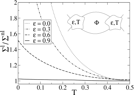
Figure 3: Ratio of the local to the non-local potential fluctuation spectrum as a function of the transmission probability ${\cal T}$ at the beam splitters for different values of $\varepsilon$. The parameter $\varepsilon$ controls the admixture of chaotic scattering. All curves are symmetric around ${\cal T}=1/2$.

In Fig. (3), the ratio of local to non-local potential fluctuations is shown for different values of the parameter $\varepsilon$. The results given there are valid in the limit of strong dephasing (as in Fig. (2)) and include an ensemble average over the random matrices ${\bf S}_{C}$ of the two intersections. From Fig. (3) it is clear that increasing the degree of chaotic scattering in the intersections suppresses the difference between the local and non-local configuration. Backscattering, on the ensemble average, thus has a similar effect as an incoherent parallel transmission $T_{0}$ between neighboring contacts. In the limit where the intersections are fully chaotic ($\varepsilon=1$), there is no difference between the local and non-local configuration. The reason is that ensemble averaging makes the ring symmetric to any measurement configuration.

In the experiment of Ref. kobayashi , the four-terminal resistance $R_{\alpha\beta,\gamma\delta}=(V_{\gamma}-V_{\delta})/I_{\alpha}$ with $I_{\beta}=-I_{\alpha}$ was measured. In terms of the conductance matrix elements, the four-terminal resistances are $R_{\alpha\beta,\gamma\delta}=\left(G_{\gamma\alpha}G_{\delta\beta}-G_{\gamma\beta}G_{\delta\alpha}\right)/D$ markus_four_term , where $D$ is any sub-determinant of rank three of the total conductance matrix. The four-terminal resistance takes a particularly simple form in the case of a reflectionless interferometer ($\varepsilon=0$) where we find

$$R_{14,23} = \frac{h}{2e^{2}}\frac{T_{0}-\langle T_{13}\rangle}{1+T_{0}-\langle T_{13}\rangle},$$ (12a)

$$R_{12,43} = \frac{h}{2e^{2}}\frac{1-2\langle T_{13}\rangle}{(T_{0}+\langle T_{13}\rangle)(1+T_{0}-\langle T_{13}\rangle)}$$ (12b)

for the local and non-local configuration, respectively. Eqs. (12a) and (12b) show that the attenuation of the local and non-local resistances is determined by the decoherence rates Eqs. (5a) and (5b) respectively.

In conclusion, we have shown that the electrical constraints imposed by the measurement circuit give rise to a probe configuration dependence of the dephasing rate. This effect is most pronounced in an ideal quantum interferometer that is strongly asymmetric, but was found to persist even in the presence of a considerable admixture of incoherent transmission or randomness (with ensemble averaging). While there may be other physical mechanisms for producing such a difference, our discussion of dephasing explicitly includes the effect of the external electrical circuit and leads to a result consistent with unanticipated experimental observations.

This work was supported by the Swiss National Science Foundation.

References

- (1) K. Kobayashi et al., J. Phys. Soc. Jpn., 71, 2094 (2002).
- (2) Y. Aharonov and D. Bohm, Phys. Rev. 115, 485 (1959).
- (3) B. L. Altshuler, A. G. Aronov and, D. Khmelnitskii, J. Phys. C 15, 7367 (1982).
- (4) M. H. Devoret et al., Phys. Rev. Lett. 64, 1824 (1990).
- (5) C. W. J. Beenakker, M. Kindermann, and Yu. V. Nazarov, cond-mat/0301476.
- (6) M. Büttiker, Phys. Rev. Lett. 57, 1761 (1986).
- (7) C. P. Umbach et al., Appl. Phys. Lett. 50, 1289 (1987).
- (8) U. F. Kayser et al., Semicond. Sci. Technol. 17, L22, (2002).
- (9) Y. Ji et al., Nature 422, 415 (2003).
- (10) M. Cassé et al., Phys. Rev. B 62, 2624 (2000).
- (11) A. E. Hansen et al., Phys. Rev. B 64, 045327 (2001).
- (12) G. Seelig and M. Büttiker, Phys. Rev. B 64, 245313 (2001).
- (13) J. P. Bird et al., Phys. Rev. B 51, 18037 (1995); D. P. Pivin et al., Phys. Rev. Lett. 82, 4687 (1999). C. Prasad et al., Phys. Rev. B 62, 15356 (2000).
- (14) R. M. Clarke et al., Phys. Rev. B 52, 2656 (1995); A. G. Huibers et al., Phys. Rev. Lett. 81, 200, (1998); A. G. Huibers et al., ibid. 83, 5090, (1999).
- (15) Y. Takane, J. Phys. Soc. Jap. 67, 3003 (1998); Y. Takane ibid 71, 2617 (2002).
- (16) AB oscillations in a MZI with two arms of equal length are not affected by thermal averaging.
- (17) M. Büttiker, H. Thomas, and A. Prêtre, Phys. Lett. A 180, 364 (1993).
- (18) If , the local dephasing rate Eq. (5a) diverges for and . The divergence has its origin in the fact that for and the two arms of the MZI become completely decoupled. It is therefore cut off by any backscattering.
- (19) M. H. Pedersen, S. A. van Langen, and M. Büttiker, Phys. Rev. B 57, 1838 (1998).
- (20) A. M. Martin and M. Büttiker, Phys. Rev. Lett. 84, 3386 (2000).
- (21) M. Büttiker, Phys. Rev. B 46, 12485, (1992).
- (22) The results Eqs. (5a), (5b) and Eq. (10) can also be extracted from the self-consistent admittance matrix seelig if the appropriate boundary conditions are used (A. N. Jordan et al., unpublished).
- (23) P. W. Brouwer and C. W. J. Beenakker, J. Math. Phys. 37, 4904 (1996).