Study of the influence of surface anisotropy and lattice structure on the behaviour of a small magnetic cluster

Abstract

We have studied by Monte Carlo simulations the thermal behaviour of a small ($N=13$ particles) cluster described by a Heisenberg model, including nearest-neighbour ferromagnetic interactions and radial surface anisotropy, in an applied magnetic field. We have studied three different lattice structures: hexagonal close packed, face centered cubic and icosahedral. We show that the zero-field thermal behaviour depends not only on the value of the anisotropy constant but also on the lattice structure. The behaviour in an applied field, additionally depends, on the different orientations of the field with respect to the crystal axes. According to these relative orientations, hysteresis cycles show different step-like characteristics.

1 Introduction

The magnetic properties of clusters have been studied intensely for about two decades. Surface and finite-size effects appear to play a key rôle for clusters containing up to several hundred atoms. An enhanced magnetic anisotropy at the surface has been observed for fine metallic particles [1] and predicted by theoretical calculations  [2, 3]. One source for this anisotropy is the difference between the coordination number at the surface and in the bulk, inducing a change in the crystal fields [2, 4, 5, 6]. It has been experimentally found that this enhancement increases as the size of the particle decreases [1].

Magnetic measurements are usually carried out by passing size selected clusters through a non uniform magnetic field as in the Stern-Gerlach experiment. In these experiments the cluster size is known but the crystal structure as well as the initial orientation of the crystal axes of the cluster with respect to the field gradient direction are not.

A great deal of effort has been devoted to the theoretical and experimental study of transition metal (TM) clusters [7, 8, 9, 10] which are known to have a relatively low anisotropy energy in the bulk compared to their exchange energy [2]. For TM clusters, it has been shown that it is the localised character of the 3d electrons at the surface which enhances the surface anisotropy with respect to the volume anisotropy [3]. On the contrary very little is known for rare earth (RE) clusters, where the anisotropy energy is expected to be higher. Experimental results on RE clusters show an anomalous behaviour (the broadening of the deflection profile in a Stern-Gerlach experiment at a finite temperature) which is absent in the case of TM clusters [11, 12].

Several studies which consider anisotropy terms have been performed, mostly concerning large clusters ($N\geq 1000$ atoms) cut to regular shapes (spherical or ellipsoidal) out of simple-cubic or spinel lattices. For these systems the competition between the surface anisotropy and the exchange term has been analysed as a function of temperature  [13, 14, 15]. The influence of surface effects on the hysteresis cycle at zero temperature has also been shown [16]. Dimitrov and Wysin [17] have studied the zero-temperature behaviour of large particles with ferromagnetically coupled Heisenberg classical spins with either uniaxial random anisotropy or radial surface anisotropy. They have studied the two-(three-)dimensional simple-cubic lattice with the cluster having either circular or rectangular (spherical or cubic) geometries. They find a step-like hysteresis cycle which is identified as a surface effect. This is also observed in their zero temperature study of spherical particles cut out of an fcc lattice structure [18]. To have a complete picture of these systems, it is of interest to investigate the thermal magnetic behaviour of small clusters, including an anisotropy energy term.

In this work we study a simple classical Heisenberg model for an $N=13$ cluster with radial surface anisotropy, at finite temperature and in an applied external field, in order to understand how the thermal magnetic behaviour of the cluster is affected by the existence of a surface anisotropy term. We will show how the interplay between the surface anisotropy and the crystal structure, as well as the relative orientation of the applied field with respect to the crystal axes, influence the magnetic behaviour of the cluster.

This article is organized as follows: in Section 2 we describe the studied systems; in Section 3 we give the technical details of our calculation, and in Section 4 we present the results. Finally, in Section 5, we summarise and discuss our results.

2 Description of the systems studied

Among the small amount of information concerning RE clusters, reference [19] shows, by ab-initio electronic structure calculations that $Gd_{13}$ clusters adopt a hexagonal closed packed (hcp) crystal structure. Numerical simulation results of cluster agregation starting from $N=13$ separated atoms placed in either Lennard-Jones or Gupta potentials yield very similar cohesion energies for hcp, fcc and icosahedral lattices [21]. These leads us to base our study on $N=13$ atom clusters having one of these three crystal structures, since the absolute values of their cohesion energies are larger than those obtained for other known simple structures (such as simple-cubic or body-centered-cubic).

Since the magnetism in RE metals comes from the localised 4f orbitals, a Heisenberg hamiltonian is a reasonable model. Different approaches exist to the treatement of the spin (classical or quantum approach) and to the interaction constants. In [19], based on the fact that the calculated Fermi energy of the band structure is in a continuum of the density of states, a classical RKKY-Heisenberg hamiltonian is considered to describe the $Gd_{13}$ cluster. On the other hand in [20] both quantum and classical approaches of a RKKY-Heisenberg hamiltonian are studied for different closed-packed N=13 clusters and for different geometries of the N=14 clusters. Concerning the thermal magnetic behaviour of the N=13 clusters, the results are qualitatively the same as in the classical approach developped in [19].

In this article we model the exchange interaction by a classical Heisenberg hamiltonian. In addition, a surface anisotropy term that acts only on the atoms at the surface to account for the reduction of the symmetry of the crystal at the surface is considered.

The main sources of anisotropy are the crystal-field anisotropy and the magnetic dipolar interaction. The latter, being a long range interaction, can in principle be neglected for small clusters. Choosing the correct term to model the surface anisotropy of a RE cluster is not an easy task as no experimental results are available. Nevertheless some hints can be taken from what is known for metallic clusters. In [1] it has been found that the surface anisotropy term increases with decreasing cluster size.

When trying to apply these results to RE clusters one can notice that first principle calculations, which concern $Gd_{13}$, [2, 19] show a contraction of the surface layers that may induce a much larger crystal field anisotropy at the surface than in the bulk. As it has been discussed in previous articles [2, 4, 5], the lowering of the symmetry at the surface due to the missing neighbours produces a crystal field with a predominant axial term in the radial direction which can be modelled by adding to the hamiltonian a term of the form $K_{s}S_{\xi}^{2}$ where $\xi$ is the component along the radial vector.

The classical RKKY-Heisenberg hamiltonian which is known to be a good model for bulk Gd [19] has been already studied numerically in a simplified version (ferromagnetic first-neighbour interactions and antiferromagnetic interactions among all other pairs) without anisotropy [23].

In this article we consider a complementary approach. Our aim is to study the influence of the surface anisotropy energy. For simplicity, as a first approach, we limit our model to the case of ferromagnetic first-neighbour couplings, the same at the surface and in the bulk, in order to avoid mixing the effects of surface anisotropy with those of competing interactions. It can be argued that for a very small particle, the spins on opposite faces of the surface are close enough to interact with each other, thus modifiying the form of the anisotropy. As in the case of the second neighbours interactions, this effect has been neglected. Since we consider clusters having an approximately spherical shape, we have also neglected the shape anisotropy.

These considerations lead to the following hamiltonian which we study for the three crystal lattices (hcp, fcc, ico):

$${\mathcal{H}}=-J\sum_{<i,j>}\vec{s}_{i}.\vec{s}_{j}-K_{s}\sum_{N_{s}}(\vec{s}_{i}.\vec{n}_{i})^{2}-\sum_{i=1}^{N}\vec{h}.\vec{s}_{i},$$ (1)

where $\vec{s}_{i}$ is a classical Heisenberg spin with unit length, $\langle i,j\rangle$ denotes the sum over all nearest-neighbour pairs, $N_{s}$ is the number of spins at the surface of the cluster (here $N_{s}=12$), $\vec{n}_{i}$ is the unit vector giving the radial direction from the central spin, $s_{1}$. $J>0$, $K_{s}>0$ and $h$ are the ferromagnetic interaction constant, the radial surface anisotropy constant, and the intensity of the applied magnetic field, measured in units of $k_{B}$ respectively. In this article we fix $J=1$.

3 Calculation details

The cluster is first simulated using standard Monte Carlo simulations for the temperature magnetic dependence of the system for the fcc, hcp and icosahedral lattices in zero field (heating and cooling simulations).

Heating and cooling cycles of the system in constant field are simulated. The different considered orientations of the applied field are depicted in figure  1. For hcp lattice these orientations are either parallel or perpendicular to the $\vec{c}$ axis of the crystal. The former is noted $\vec{H}_{c}=h\vec{u}_{c}$ and the latter $\vec{H}_{n}=h\vec{u}_{n}$, where $\vec{u}_{n}$ is a basis vector of the hexagonal central layer. As the fcc lattice can be seen in a layered way, the same definition of the direction of the applied field as in the hcp structure is used (see figure 1.b). For the icosahedral structure, the $\vec{u}_{c}$ orientation is chosen along the direction of one of the 5-fold symmetry axes. The complementary $\vec{u}_{n}$ direction is perpendicular to $\vec{u}_{c}$ and joins the intersection point, noted S, of the 5-fold axis with the perpendicular plane containing the 5 icosahedral sites, with one of these sites (see figure 1.c). Hysteresis cycles are simulated at different temperatures, with the magnetic field applied in the predefined directions of each structure.

Figure 1: Studied lattice structures, definition of $\vec{u}_{c}$ and $\vec{u}_{n}$ directions of the applied field for the field cooling and hysteresis simulations. (a) hcp, (b)fcc, (c) icosahedral lattices.

All these simulations are done using $10^{6}$MCS/s steps for calculation after having discarded $10^{6}$MCS/s steps for the thermalisation process. Quantities are averaged using one configuration every 100MCS/s in order to diminish statistical correlations.

We define the average cluster magnetisation as

$$m=1/N<|\sum_{i=1}^{N}\vec{s}_{i}|>,$$ (2)

and the average surface magnetisation of the cluster,

$$m_{s}=1/N_{s}<\sum_{N_{s}}|\vec{s}_{i}.\vec{n}_{i}|>,$$ (3)

The energy is also calculated as a function of the temperature and the magnetic field.

4 Results

4.1 Charaterisation of the ground states

In order to have a better understanding of the effect of surface anisotropy at finite temperature and in an applied field, it is necessary to have an idea of the ground state of the model for the different lattice structures in zero field. Unfortunatelly, the analytical determination of the ground state of this hamiltonian is not straightforward. The coupling between the spins and the crystal structure makes it impossible to perform a reduction of the number of variables in the problem by a global rotation of the magnetic structure. Moreover, as this coupling is non-linear, one can not use the local field orientation search methods for the ground state. We search for the ground state numerically using simulated-annealing, with a decreasing power law for the temperature: $T_{i+1}=(T_{i})^{\alpha}$, where ”i” labels the cooling step and $1.05<\alpha<1.15$.

We obtain ground-state magnetisations $m(0)<1$ for the three considered lattices due to the surface anisotropy term, which favors a canted low temperature configuration. This non-collinear order is confirmed by the surface average magnetisation which saturates near $m_{s}(0)\approx 1$ for big enough values of $K_{s}$.

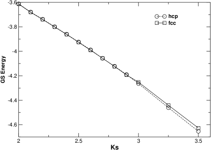
Figure 2: Ground-state energy as a function of $K_{s}$ from simulated annealing for the hcp and fcc lattices.

We note a qualitative difference between the ground-state behaviour of the hcp and fcc clusters and that of the icosahedral cluster. The ground-state energies and magnetisations of the hcp and fcc clusters are very close for low anisotropy and start to differ for a value around $K_{s}=3$, while the corresponding energy and magnetisation values are very different for the icosahedral cluster. Figure 2 shows the ground-state energies for the two structures having the closest behaviour in the interesting region of the anisotropy, $2<K_{s}<4$.

Figures 3 and 4 illustrate schematically the ground-state configurations found for the hcp and fcc structures for $K_{s}=3$, where the two lattices start to differ. For the hcp lattice we find two degenerate ground states corresponding to two different values of the magnetic moment. For the fcc cluster, only one magnetisation state is found.

Two typical low temperature configurations of the hcp lattice are represented in figures 3(a) and  3(b). In figures 3(c) and  3(d) their projections on the central plane may be seen (for clarity, we draw the spin orientations along the radial directions; the real spin configurations show slight deviations from these directions). The magnetic moment of the cluster (shown in figure 3(a)), corresponding to the ground state with the higher magnetisation, is mainly aligned along $\vec{u}_{c}$, while for the case of the lower magnetisation ground state (given in figure 3(b)), the magnetic alignement is mainly along $\vec{u}_{n}$.

In figure 4(a) we show a typical ground-state configuration of the fcc lattice. This configuration has the same magnetic moment as the hcp ground state with the higher magnetisation (figure 3(a)). And as for this hcp ground state, the main direction of the magnetic moment is along $\vec{u}_{c}$.

In order to understand why the ground state is not degenerate for the fcc cluster while it is degenerate for the hcp cluster, we impose the low temperature spin configuration found for the hcp lattice, shown in figure 3(b), to the fcc lattice (respecting all the possible symmetries). This “non-physical” configuration is shown figure 4(b). Comparing figures 3(d) and  4(d), it becomes clear why the ground-state configuration with the lower magnetisation in the hcp is not found in the fcc cluster: the coupling between the spins in the central plane and those in the lower plane increases the energy in the case of the fcc structure.

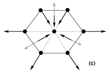
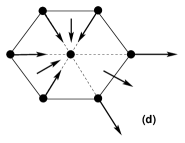
Figure 3: Typical ground-state configurations for the hcp lattice for $K_{s}=3$. Dotted lines indicate the radial directions. The real configurations show a slight deviation from the radial directions which we haven’t drawn here for simplicity. The central spin is irrelevant (it follows orientation of the majority of its in-plane neighbours) and is not shown here for the sake of clarity. (a) Ground state corresponding to the case with the higher magnetic moment (mainly aligned along $\vec{u}_{c}$). (b) Ground state corresponding to the case with the lower magnetic moment (mainly aligned along $\vec{u}_{n}$). (c) Projection of configuration (a) on to the central plane; thick arrows indicate the upper plane projections and thin arrows those of the lower plane. (d) Projection of configuration (b) on to the central plane; upper and lower planes projections are coincident.

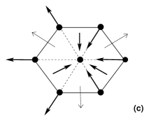
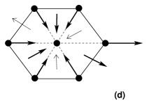
Figure 4: Typical ground-state configurations for the fcc lattice for $K_{s}=3$. Dotted lines indicate the radial directions. The real configurations show a slight deviation from the radial directions which we haven’t drawn here for simplicity. The central spin is irrelevant (it follows orientation of the majority of its in-plane neighbours) and is not shown here for the sake of clarity (a) Ground-state configuration ; it has the same magnetic moment than the hcp ground-state configuration (with the highest magnetic moment) given in figure 3(a). (b) ”Non-physical configuration” obtained imposing the other hcp ground-state configuration (with the lowest magnetic moment) given in figure 3(b) to the fcc lattice ; the energy of such a configuration is much higher than the energy of (a). (c) Projection of configuration (a) on to the central plane. (d) Projection of configuration (b) on to the central plane ; thick arrows indicate the upper plane projections and thin arrows those of the lower plane.

As $K_{s}$ increases, the degeneracy of the hcp ground state is lifted in favour of the most canted ground state, i.e. with a lower magnetisation than the ground state of the fcc cluster, and the ground states of the fcc and hcp lattices separate in energy and in magnetisation. The hcp cluster is better able to minimize both exchange and surface energy.

The low temperature behaviour of the icosahedral cluster always differs from the other two structures. The magnetic moment values $m(0)$ of the icosahedral lattice at a given value of the anisotropy constant $K_{s}$ are higher than those of the other two structures in all the anisotropy range considered. This can be understood by the different number of nearest neighbours at the surface. The sites at the surface of both hcp and fcc lattices have 5 nearest neighbours while the sites of the icosahedral lattice have 6. At fixed $K_{s}$, the ferromagnetic coupling favours ground-state configurations with higher magnetisations in the icosahedral cluster than in the other two, in agreement with our results (see figure 5). And the ground-state energies of the icosahedral lattice are much lower than the corresponding energies for hcp and fcc lattices. This is due to the globular geometry of the icosahedral cluster that allow a better compromise to minimize both exchange and surface energy.

Figure 5: Schematical ground-state configuration for the icosahedral lattice for $K_{s}=3$. Dashed lines indicate radial directions. For the sake of clearness, we draw the spins fully oriented along the radial directions in spite of the fact that the actual configurations show a slight deviation from the directions shown here. This deviation tends to align all the spins along the vertical $C_{5}$ axis, increasing the magnetisation with respect to the one of the pure radial configuration.

We will see that the similarities of both hcp and fcc clusters, as well as the specificities of the icosahedral cluster that we pointed out in this section, will be emphasized by the action of temperature or the application of an external magnetic field.

4.2 Zero field thermal behaviour

We have performed heating and cooling cycles for the three considered lattices structures in a range of values of the anisotropy constant $1\leq K_{s}\leq 7$. Figure 6 shows the average magnetisation of the particle in a cooling process in zero field for different $K_{s}$ values and the three considered lattice structures.

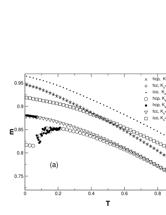
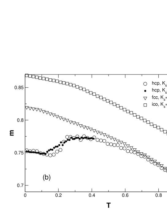
Figure 6: Magnetic moment as a function of temperature for hcp, fcc and icosahedral lattice structure. Zero-field cooling simulations. Full symbols indicate a slow cooling. (a) $K_{s}$=2 and 3. In a slow field cooling process for the hcp lattice with $K_{s}$=3, the magnetisation decreases when lowering $T$ and suddenly increases again to rejoin the fcc curve for the same $K_{s}$. The two low $T$ states shown have the same energy. (b)idem, $K_{s}$=4, the slow cooling process doesn’t modify the peak and the saturation value of m is lower than for finite $T$.

The influence of surface ansitropy on the temperature behaviour of the magnetisation clearly depends on the crystal structure. For $K_{s}=2$ the $m(T)$ curves increase monotonically for the three structures. The $m(T)$ curve of the icosahedral lattice is higher than those of the two other structures in all the measured temperature range.

For $K_{s}=3$ the degenerate ground state of the hcp structure leads to a $m(T)$ curve showing an anomalous behaviour. Which of the ground states is reached depends on the trajectory performed in the phase space while cooling the system. As the temperature is lowered, the magnetisation of the cluster grows, but at a value $T_{a}$ it rapidly falls down creating a peak (open circles in figure 6). If the cooling process is performed very slowly, the cluster magnetisation first decreases and then increases again reaching the same low temperature value of the magnetic moment than for the fcc structure (full circles in figure 6). Energy curves $E(T)$ of the two runs (not shown here) superpose exactly, and superpose also to the $E(T)$ curves of the fcc cluster. Obviously, for the fcc where no degeneracy has been found, the behaviour of the $m(T)$ curves doesn’t show any dependence on the trajectory in the phase space during the zero-field cooling proccess. As expected, the two $m(0)$ values of figure 6 for hcp and fcc lattices correspond to the magnetisation ground states found in figures 3 and 4.

When performing a standard MC zero-field cooling simulation of the hcp lattice starting from the low magnetisation ground states found by simulated annealing for $K_{s}=3$, the zero-field cooling curves are reproduced exactly and the peak shown in figure 6(a) appears again.

As we have discussed in the previous section, as $K_{s}$ increases, the degeneracy of the hcp ground state is lost and the ground states of the fcc and hcp lattices separate in energy (see figure 2). For instance, for the hcp cluster and $K_{s}$=4, the peak is always found when cooling the system and as expected, the saturation value of the cluster magnetisation is smaller than for the fcc structure (figure 6(b)). Increasing $K_{s}$ diminishes the height of the peak till it disappears. This behaviour is a particularity of the hcp structure.

For the other lattice structures the cluster magnetisation increases monotonically when cooling and only for big values of $K_{s}$ a plateau is observed.

In all the cases the $m(T)$ curves are ordered (from highest to lowest case) as follows: icosahedral, fcc and hcp. This fact shows that, at fixed $K_{s}$, a different degree of competition appears between the exchange and the surface term according to the considered lattice structure. We will see this fact emphasized by the application of an external magnetic field.

4.3 Non-zero field thermal behaviour

We simulated the field cooling of the system with the field applied in directions described in figure 1. We studied various intensities of the field ranging from $0\leq h\leq 1$.

Figure 7(a) shows $m(T)$ for $K_{s}$=3 and the two considered orientations of $\vec{H}$. When the field is $\vec{H}_{c}=h\vec{u}_{c}$ ($h\geq 0.05$) the magnetisation grows monotonically as the temperature is decreased, and the anomaly observed in zero field disappears. On the contrary, when the field is pointing in the $\vec{u}_{n}$ direction, a peak is observed for the same $T\approx T_{a}$ where the anomaly is found in zero field. This peak is confirmed by a very slow cooling process as reported in figure 7(a). Obviously, when the applied field is too high the peak is destroyed, and the magnetisation grows monotonically as $T$ is lowered.

The ground-state analysis of section 4.1 helps to understand why this is so. As decribed above, two degenerate states are found for the hcp lattice for $K_{s}=3$ and $h=0$: one corresponding to the monotonous $m(T)$ behaviour (figure 3(a)) and another one corresponding to the peak in $m(T)$ curves (figure 3(b)). The former has its magnetic moment mainly oriented along $\vec{u}_{c}$ and the latter mainly along $\vec{u}_{n}$. Then when the magnetic field is applied, one of these degenerate zero-field ground states is selected according to the orientation of the field. For the fcc lattice, on the other hand, only one possibility exists (figure 4(a)) and the $m(T)$ curves do not depend on the field direction.

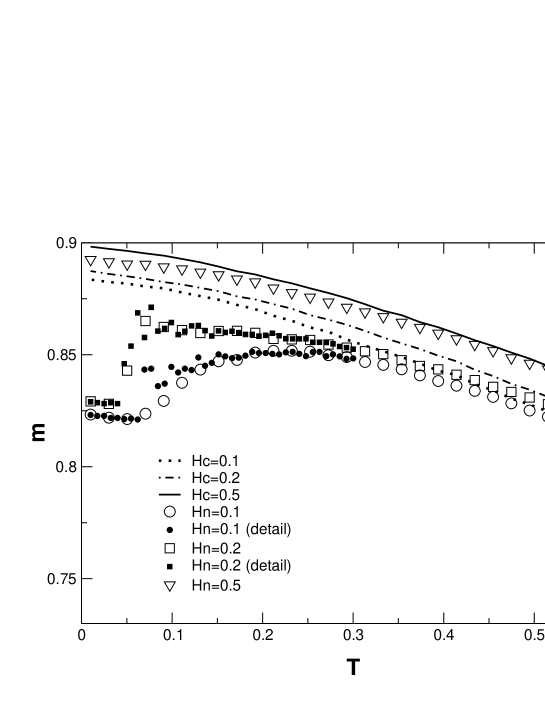
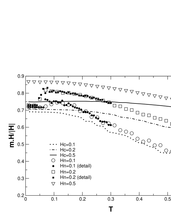
Figure 7: Hcp lattice, $K_{s}$=3. Field-cooling simulations. $H_{c}$ and $H_{n}$ denote the magnetic field intensities along the directions described in figure 1(a). Full symbols curves, issued from slow field-cooling simulations, show that the peak is stable. (a) Magnetic moment as a function of temperature. (b) Projection of the magnetisation along the axis of the corresponding applied field.

In figure 7(b) we plot $|\vec{m}.\vec{H}|/|\vec{H}|$ as a function of $T$ for different intensities and the two studied orientations of the applied field. It can be seen that the behaviour of the corresponding projection of the average magnetisation along the field direction depends on this direction. When the field is applied along $\vec{u}_{n}$ the corresponding projection of the average magnetisation, called $m_{n}$, easily follows the field as $T$ is lowered. However when the field direction is $\vec{u}_{c}$ the corresponding projection, $m_{c}$, grows very slowly as $T$ is lowered saturating for $T<T_{a}$.

Comparing figure 7(a) and (b) one can understand the difference in the magnetic behaviour between the two chosen field directions. When the field is in the $\vec{u}_{c}$ direction, the magnetic moment grows monotonically (the peak observed in zero field disappears) while the $m_{c}$ projection saturates at value lower than one at finite $T$. This means that there is a non zero contribution to the magnetic moment which is not in the $\vec{u}_{c}$ direction. The situation is different when the field is in the $\vec{u}_{n}$ direction, we can see that it is mainly $m_{n}$ which is responsible for the peak on the $m(T)$ curve.

For the fcc structure the behaviour is different. To compare with the hcp lattice we considered the field directions as shown on the figure 1(b). The $m(T)$ curves are coincident for both directions of the applied field and no anomaly is observed (see figure 8(a)). This result remains true for all field intensities and for all values of $K_{s}$. This can be understood in terms of the structure of the ground state: for the fcc lattice there’s no degeneracy of the ground state so the $m(T)$ curves do not depend on the field direction. On the other hand, as for the hcp lattice, when the field is applied in the $\vec{u}_{n}$ direction, $m_{n}$ follows the field more easily than does $m_{c}$ when the field is applied in the $\vec{u}_{c}$ direction (see figure 8(b)). The zero-temperature value of $m_{c}$ is lower than the corresponding one for $m_{n}$ for all $K_{s}$, also in agreement with the hcp case. This can also be related to the characteristics of the ground-state configurations in zero-field (figures 3 and 4): in both hcp and fcc ground states we have found that the spins in the central plane have a small component along the $\vec{u}_{c}$ direction, so, when a magnetic field is applied along $\vec{u}_{c}$, the spins in the central plane find it more difficult to align with the field direction.

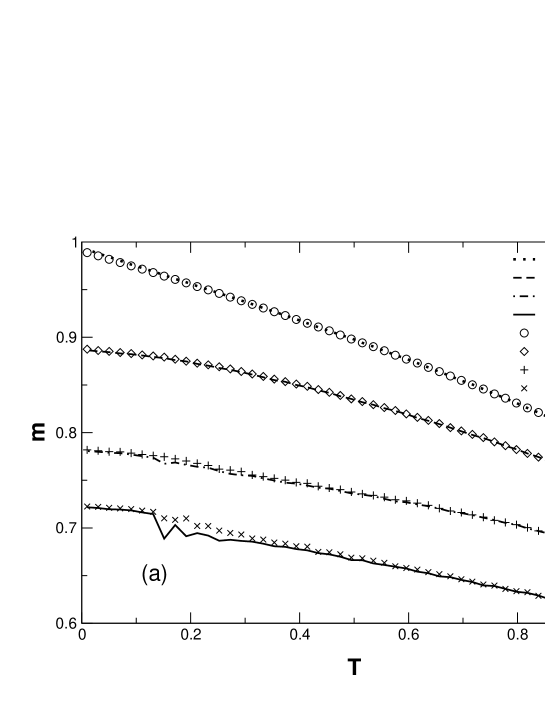
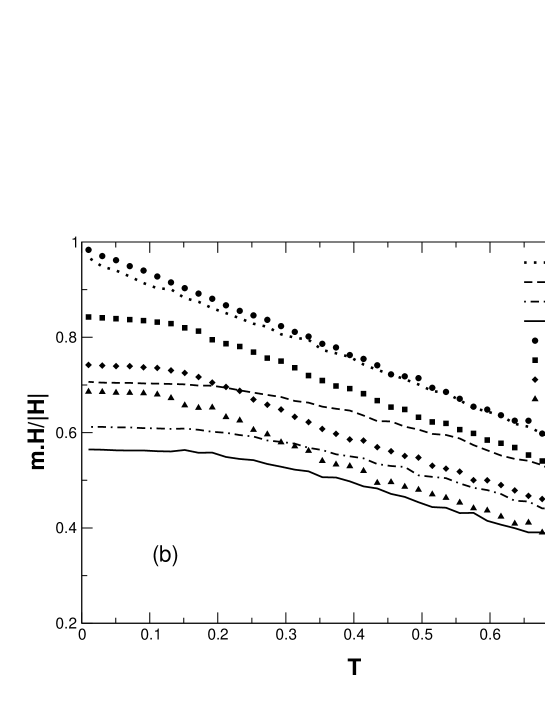
Figure 8: Fcc lattice, the intensity of the applied field is $h=0.2$. Field cooling simulations. $H_{c}$ and $H_{n}$ denote the applied magnetic field parallel to the $\vec{u}_{c}$ and to the $\vec{u}_{n}$ axis respectively (see figure 1(b)). (a)The magnetic moment as a function of temperature is not affected by the direction of the applied field for all $K_{s}$ values. (b) Projection of the magnetisation along the direction of the corresponding applied field. For all $K_{s}$ values, the magnetisation follows the field more easily when it is applied along the $\vec{u}_{n}$ axis.

The situation for the icosahedral lattice is less straightforward. First, this lattice has a globular structure rather than the layered structure of hcp or fcc, and so, one cannot directly identify the 5-fold symmetry with the $\vec{u}_{c}$ axis of the other two layered structures. Nevertheless, the results of field cooled simulations show, as for the fcc case, that the orientation of the field has no influence in the $m(T)$ curves. On other hand, the orientation of the field affects the projection of the magnetisation in the field direction (see figure 9). For this structure, it is $m_{c}$ which follows more easily the applied field. For $K_{s}\geq 3$ $m_{c}$ reaches its saturation value at a finite value of $T=T_{s}$. This value increases with $K_{s}$. This is also a sign of a non-collinear state, confirmed by the high values of the surface magnetisation at zero temperature ($m_{s}(0)\geq 0.9$ for $K_{s}\geq 6$).

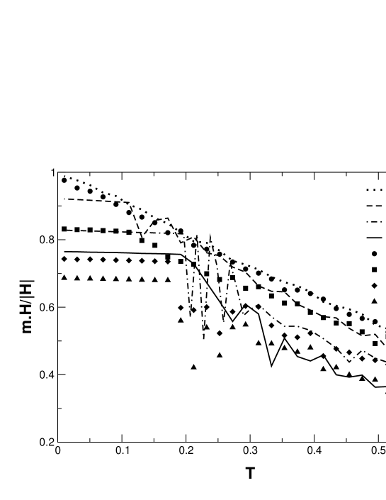
Figure 9: Icosahedral lattice, the intensity of the applied field is $h=0.1$. Field cooling simulations. $H_{c}$ and $H_{n}$ denote the magnetic field applied parallel to the $\vec{u}_{c}$ and to the $\vec{u}_{n}$ axis respectively (see figure 1(c)). A plateau appears at $T=T_{s}$ ($T_{s}$ increases with $K_{s}$). For high values of $K_{s}$ ( $K_{s}>5$) large fluctuations are observed just before the plateau.

For a given lattice and a fixed value of the field intensity $h$, two different regimes are observed for the thermal behaviour of magnetic moment, $m(T)$, and of the projection of the magnetisation of the surface spins along the radial directions $m_{s}(T)$, according to the value of $K_{s}$. For low $K_{s}$, $m(T)$ is higher than $m_{s}(T)$ for all $T$. For high $K_{s}$ values, the opposite behaviour is observed. There is then a range of $K_{s}^{c}$ values where the two curves cross at a finite temperature, $T_{cross}(h)$, leading to a non-collinear ground state ($m_{s}(0)>m(0)$). In spite of the fact that one cannot actually talk of a phase transition, this crossing indicates that the non-collinear state, where each magnetic moment has a strong component perpendicular to the surface, takes over from a state of large global magnetisation (collinear state). The range of $K_{s}^{c}$ values is characteristic of each lattice structure. For the studied values of $K_{s}$, we have found $K_{s}^{c}\approx 4$ for hcp and fcc and $K_{s}^{c}\approx 5$ for the icosahedral structure. This dependence of the $K_{s}^{c}$ is related to the different number of nearest neighbours at the surface for the different structures. As already mentioned, the sites at the surface of both hcp and fcc lattices have 5 nearest neighbours while the sites of the icosahedral lattice have 6, which leads to a larger $K_{s}^{c}$ in this latter case so as to counterbalance the ferromagnetic coupling.

We have studied the $T_{cross}(h)$ dependence for a given lattice at the corresponding $K_{s}^{c}$ values, when the field is applied along the $\vec{u}_{c}$ direction (highest symmetry axis for the three lattices). We observe that $T_{cross}(h)$ shifts to low temperatures as the applied field increases. This simply reveals the fact that when a field is applied, the thermal energy needed to flip from the non-collinear to the collinear state is lower. In the case of very high fields, $T_{c}(h)\to 0$, indicating that the ground state is already collinear.

4.4 Hysteresis loops.

Starting from a zero-field cooling state, we performed hysteresis loops with the field oriented along each of the directions described above. We observe that above the temperature $T_{a}$ corresponding to the anomaly of the hcp lattice, no hysteresis is found. Then, to allow for comparison, we performed for all the lattices the hysteresis cycles at $T\leq 0.1$, where the hysteresis is found in hcp structure.

For the hcp lattice no hysteresis loop is observed for $K_{s}$=1 but it is already present for $K_{s}$=2. We observe that the field orientation along $\vec{u}_{c}$ gives a smoother loop than the orientation along $\vec{u}_{n}$ for all $K_{s}$ values. In Figure 10(a) it can be seen that small plateaux, and a larger coercive field, appear when the field is applied along the $\vec{u}_{n}$ direction.

For $K_{s}$=3 these characteristics persist (see Figure 10(b)). Hysteresis disappears only in the $\vec{u}_{c}$ direction for $K_{s}$=4 and for both directions for $K_{s}$=5.

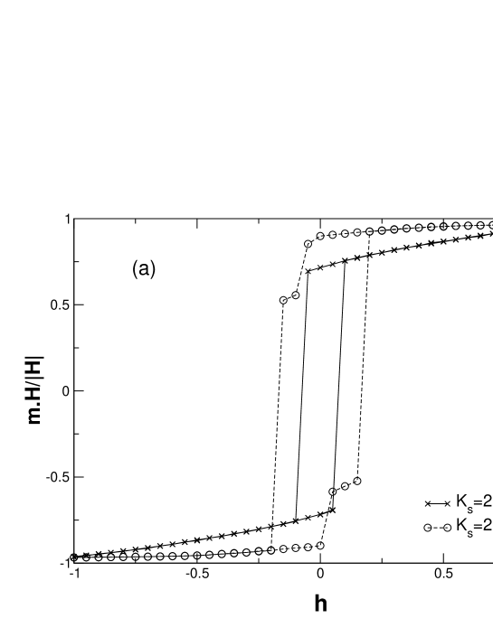
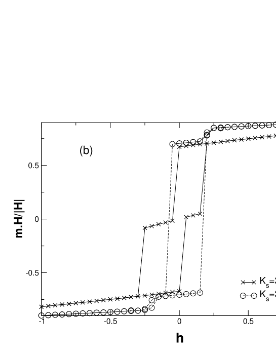
Figure 10: Hcp lattice, hysteresis cycle, $T=0.01$. $H_{c}$ denotes the magnetic field applied parallel to the $\vec{u}_{c}$ axis, $H_{n}$ denotes the magnetic field parallel to the $\vec{u}_{n}$ axis (see figure 1(a)). Projection of the magnetisation along the axis of the corresponding applied field. The lines are only a guide to the eye. (a) $K_{s}$=2, (b) $K_{s}$=3. The cycle width is larger when the field is parallel to the $\vec{u}_{n}$ axis. In this case the magnetisation remains almost unchanged till $h=0$, showing intermediate jumps before saturating on the opposite sens. When the field is parallel to $\vec{u}_{c}$ a monotonous increase of the magnetisation with the applied field can be observed.

For the fcc lattice the dependence of the coercive field on the orientation of the applied field is the same as for hcp, but the cycle width starts diminishing already at $K_{s}$=3.

For these two lattices, the magnetisation shows small plateaux as a function of the applied field. Step-like hysteresis cycles have been observed for large clusters with surface anisotropy in [16, 17, 18] and for small antiferromagnetic clusters in [22]. They have been explained in terms of the simultaneous reversal of a group of spins. Here we show, additionally, that the location of these plateaux depends not only on the intensity of the field but also on its direction with respect to the crystal axes of the clusters.

For the icosahedral lattice the situation is once again different from that of the layered structures. First, at the temperature where we performed the previous field loops, the MC simulation fails to flip individual spins over the high energy barriers. This different temperature scale is again due to the higher coordination of the surface sites, which increases the effect of the ferromagnetic coupling. We have then performed the field loops at $T=0.1$ (the hysteresis disappears for $K_{s}$=3 at $T=0.15$). Second, at a given $T$, the width of the hysteresis loops increases with $K_{s}$, which indicates that it is more difficult to reverse the magnetisation of the system as $K_{s}$ increases, in contrast with the hcp and fcc cases. Again, this can be understood considering the peculiarities of this globular structure, and comparing its ground state with those found for hcp and fcc (see figures 3, 4 and 5). For a layered lattice one can see that there is a competition between the field and the anisotropy terms: when the cluster is (almost) completely polarized, for exemple, in the $+\vec{u}_{c}$ direction, the anisotropy term in the hexagonal layer is far from being optimized (it is globally zero); when the field is then diminished in the reversal process, the anisotropy term “helps” the individual spin transitions. The situation is different for the icosahedral structure in which the radial character of the anisotropy term allows for a configuration which can follow the field without rising too much the anisotropy energy. When the field is reversed at low $T$, again in order to satisfy both terms, each individual spin must completely reverse its orientation along its radial direction, so the intermediate states involve a jump over the anisotropy barrier, which increases with $K_{s}$. This is exactly what we observe, the coercive field increases with $K_{s}$. We thus believe that the single spin flip algorithm used is not adapted for the study of low temperature hysteresis loops for the icosahedral cluster.

5 Conclusions

We have studied the magnetic thermal behaviour of a $N=13$ cluster in a magnetic field. We have considered a classical Heisenberg model with ferromagnetic interactions in a magnetic field, and a radial surface anisotropy term. This model has been applied to three different lattice structures, hcp, fcc and icosahedral, which have similar cohesion energies in the context of Lennard-Jones and Gupta potentials.

Our results show that, even in zero field, the crystal structure of the cluster plays an essential role on its thermal behaviour. In particular, the anomalies seen in the average cluster magnetisation curves as a function of the temperature for some surface anistropy constants seems characteristic of the hcp structure.

This anomalous magnetic behaviour has been observed on $Gd_{13}$ clusters  [12] which are found to present a hcp structure [19]. Experimental measurements of the magnetic moment per atom of $Gd_{13}$ clusters give values well below the one predicted by electronic structure calculations for the ground state of the $Gd_{13}$ [19] and show a peak in the $m(T)$ curves [12, 20].

It has been proposed that a non-collinear arrangement of the atomic moments could be responsible for such a behaviour [12, 19]. In  [19] a simplified version of a RKKY model, with no anisotropy term, is proposed as a way to obtain these non-collinear configurations. In fact, the oscillating character of the RKKY interactions has been replaced by a ferromagnetic nearest-neighbour interaction and an antiferromagnetic coupling of all other pairs in the cluster, thus renforcing the competition. In [23], using the same model on a hcp lattice, the authors find a range of values for the competing ratio between ferromagnetic and antiferromagnetic interactions, $\gamma$, where the $m(T)$ curves in zero field have a peak. These two studies use a classical approach.

On the other hand, in [20] a classical and a quantum study of the model has been carried out. In this case they consider competing interactions: ferromagnetic between first neighbours and antiferromagnetic only between second neighbours. They study N=13 atom closed packed clusters with: body centered cubic, face centered cubic, hexagonal compact packing and icosahedral structures. They also study the N=14 hcp (open shell) cluster with different geometries. For the closed packed (N=13) clusters, the results of the quantum approach are qualitatively the same as those of the classical one found in [19, 23]. In all these studies the behaviour of the $m(T)$ curves is the same: they show a peak where the difference $\delta m=m(T_{max})-m(0)$ is less than $10\%$ of the maximum value ($m(T_{max}$).

In this paper, we show that the same qualitative behaviour may be induced by a simple hamiltonian including, in addition to the first neighbours ferromagnetic interaction, a radial surface anisotropy term which accounts for a reduction of the symmetry of the crystal at the surface. Our results show that, for the hcp structure, the one which $Gd_{13}$ is assumed to have [19], the competition between the two energy terms leads to a peak in the $m(T)$ curves for a certain range of $K_{s}$. For the same range of $K_{s}$ the low temperature magnetisation is decreased and a non-collinear configuration appears, in qualitative agreement with the experimental results [12]. The $\delta m$ value we found is of the same order than in the previous works.

In these two complementary approaches the constants of the model are over-estimated. In our case the values of $K_{s}$ leading to the peak are too big compared to the first neighbour interaction. In the RKKY approach (classical or quantum) the antiferromagnetic interaction intensity necessary to observe the peak is about $36\%$ of the ferromagnetic one. This is around one order of magnitude higher than the ratio between the first and the second peaks of the RKKY interaction. In [23] this is additionnaly over-estimated by the fact that all the neighbours but the nearest are coupled antiferromagnetically with the same intensity.

In real RE clusters one can expect both effects (competing RKKY interactions and surface anisotropy) to be present. They both contribute to the non-collinear order and this may allow for the peak in the $m(T)$ curves to be observed for more realistic values of $K_{s}$ and $\gamma$ than those used in all these works. It is also useful to notice that for small clusters the experimental estimations of Curie temperature are much bigger than for the bulk. For instance, for $Gd_{13}$ it has been found $T_{c}>500K$ when bulk Gd Curie temperature is $T_{c}^{\it bulk}=293K$ [12]. This means that the cluster is able to maintain its magnetic order well beyond the temperature corresponding to the bulk. This pleads for a model which could be compatible with a canted structure and a stabilisation of magnetic order even for quite high temperatures. The antiferromagnetic second order interaction in competition with the first neighbours one goes in the sense of a lowering of the $T_{c}$. On the contrary, the anisotropy term contributes to stabilize a canted magnetic structure. This suggests that a more realistic model should include both therms in the hamiltonian.

In a Stern-Gerlach experiment, the projection of the magnetisation of a single particle along the field gradient direction is measured. We have shown that this projection depends on the relative orientation between the applied field and the crystal axes. Then, different relative orientations, experimentally unknown, will broaden Stern-Gerlach deflection profiles. Such broadened deflection profiles have been observed for some RE clusters [12]. In this case, it is said that the clusters have a locked moment behaviour [11, 12]. This means that the individual spins of the cluster are tightly coupled to the lattice by the crystal anisotropies, finding it more difficult to follow the applied field. This gives rise to broad deflection profiles. We show additionally, that the relative orientation of the applied field with respect to the crystal axes of the cluster also contribute to the broadening of the deflection profiles.

We want to stress that, in this work, we deal with equilibrium properties of the clusters, so we are not describing the relaxation process taking place in Stern-Gerlach apparatus. This relaxation should be considered in the interpretation of the results of such experiments. This has been done by an intermediate approach, besides the superparamagnetic model and locked-moment model, in both semiclassical [24] and quantum version [25]. These models consist in treating the cluster as a single magnetic moment coupled to the crystal by an uniaxial volume anisotropy term and to the applied field. The rotation degrees of freedom allow for the cluster’s magnetic moment relaxation. This approach is complementary to ours. The anisotropy term is different and will not give the canted spin structure proposed for $Gd_{13}$ [19]. In addition, it does not describe the competition between exchange and anisotropy energies since it does not allow for individual relaxation of the spins. So no dependence on the lattice structure can be obtained within this approach.

Hysteresis cycles at low temperature also show a dependence on the lattice structure and surface anistropy as well as on the direction of the applied field.

Our results show that the effect of the lattice structure on the magnetic behaviour cannot be neglected. Moreover, as the crystalline structure is not known for general N (first principles results are available only for very small particules), it is not excluded that, at the temperatures of the experiment, different structures could be present for a given N. Again, the different values of the low-temperature magnetisation could broaden the deflection profile.

Most of our results are related to the fact that, for small clusters, the structural details become important. Authors studying very large clusters focus mainly on the shape of the cluster which is cut out of a lattice having simple cubic (or spinel) lattice structure. In these studies, it is shown how the surface anisotropy contributes to the existence of steps in the hysteresis loops. No anomaly in the $m(T)$ curves has been reported (see [13]). Nevertheless, when N increases, the ratio of the number of spins at the surface to the total number of spins decreases and the second neigbours energy increases. It is then interesting to consider a model taking into account at the same time competing interactions and surface anisotropy to study how these properties evolve with N. This study is in progress.

References

- [1] F. Luis, J. M. Torres, L. M. García, J. Bartolomé, J. Stankiewicz, F. Petroff, F. Fettar, J. L. Maurice and A.Vaurès, Phys. Rev. B 65 (2002), p094409.
- [2] P. V. Hendriksen, S. Linderoth, P.-A. Lindgard, Phys. Rev. B 48 (1993), p7259; P.-A. Lindgard, P. V. Hendriksen, Phys. Rev. B 49 (1994), p12291.
- [3] G.M. Pastor, J. Dorantes-Dávila, S. Pick, H. Dreyssé, Phys. Rev. Lett. 75 (1995), p326.
- [4] R. H. Kodama and A. E. Berkowitz, Phys. Rev. B 59 (1999), p. 6321.
- [5] A. Aharoni, Introduction to the Theory of Ferromagnetism Second Edition, (Oxford University Press, 2000), Chapter 5.
- [6] D. A. Garanin and H. Kachkachi, Phys. Rev. Lett. 90 (2003), p. 065504.
- [7] J. P. Bucher and L. A. Bloomfield, Int. Journal of Modern Physics B 7 (1993) p 1079 and references therein.
- [8] I. M. L. Billas, A. Châtelain, W. A. de Heer, Science 265 (1994), p1682; I. M. L. Billas, A. Châtelain, W. A. de Heer, Phys. Rev. Lett. 71 (1993), p4067; Isabelle M. L. Billas, A. Châtelain, W. A. de Heer, J. Magn. Magn. Mater. 168 (1997), p64.
- [9] J. Merikoski, J. Timonen, M. Manninen, Phys. Rev. Lett. 66 (1991), p938.
- [10] J. P. Bucher and L. A. Bloomfield, Phys. Rev. B 45 (1992), p2537.
- [11] D. C. Douglass, J. P. Bucher and L. A. Bloomfield, Phys. Rev. Lett. 68 (1992), p1774; D. C. Douglass, A. J. Cox, J. P. Bucher and L. A. Bloomfield, Phys. Rev. B 47 (1993), p12874.
- [12] Danièle Gerion, Armand Hirt, and André Châtelain, Phys. Rev. Lett. 83 (1999), p532 and references therein.
- [13] H. Kachkachi, M. Noguès, E. Tronc and D. A. Garanin, J. Magn. Magn. Mater. 221 (2000), p158.
- [14] H. Kachkachi, A. Ezzir, M. Noguès and E. Tronc, Eur. Phys. J. B 14 (2000), p681.
- [15] Y. Labaye, O. Crisan, L. Berger, J. M. Greneche and J. M. D. Coey, J. of Appl. Phy91 (2002), p8715.
- [16] H. Kachkachi and M. Dimian, Phys. Rev. B 66 (2002), p174419.
- [17] D. A. Dimitrov and G. M. Wysin, Phys. Rev. B 50 (1994), p3077.
- [18] D. A. Dimitrov and G. M. Wysin, Phys. Rev. B 51 (1995), p11947.
- [19] D. P. Pappas, A. P. Popov, A. N. Anisimov, B. V. Reddy and S. N. Khanna, Phys. Rev. Lett. 76 (1996), p4332.
- [20] F. López-Urías, A. Díaz-Ortiz, and J. L. Morán-López, Phys. Rev. B 66 (2002),p144406.
- [21] S. Sugano, Microcluser Physics, (Springer Series in Materials Science Vol 20, ed. by J P Toennies, Springer Verlag, Berlin, Heidelberg, 1991), Chapter 2 (and references therein).
- [22] E. Viitala, J. Merikoski, M. Manninen, J. Timonen, Phys. Rev. B 55 (1997), p11541.
- [23] V. Z. Cerovski, S. D. Mahanti and S. N. Khanna, Eur. Phys. J. D 10 (2000), p119.
- [24] P. J. Jensen and K. H. Bennemann, Z. Phys. D 29 (1994), p67.
- [25] N. Hamamoto, N. Onishi, G. Bertsch, Phys. Rev. B 61 (2000), p1336 and references therein.