Alternative model of the Antonov problem

Abstract

Astrophysical systems will never be in a real Thermodynamic equilibrium: they undergo an evaporation process due to the fact that the gravity is not able to confine the particles. Ordinarily, this difficulty is overcome by enclosing the system in a rigid container which avoids the evaporation. We proposed an energetic prescription which is able to confine the particles, leading in this way to an alternative version of the Antonov isothermal model which unifies the well-known isothermal and polytropic profiles. Besides of the main features of the isothermal sphere model: the existence of the gravitational collapse and the energetic region with a negative specific heat, this alternative model has the advantage that the system size naturally appears as a consequence of the particles evaporation.

I Introduction

Thermodynamical properties of selfgravitating systems are very different from the ones exhibited by the traditional systems. They are typical nonextensive systems since they are nonhomogeneous and the total energy is not extensive, which is a consequence of the long-range character of gravitational interaction. They also exhibit energetic regions with a negative specific heat, which persist even in the thermodynamic limit pad ; kies ; ruelle ; lind ; antonov ; Lynden ; Lynden1 ; thirring . That is the reason why the Gibbs canonical ensemble is non applicable to the description of selfgravitating systems, since this ensemble is not able to access to those macroscopic states possesing a negative heat capacity. At first glance, the selfgravitating systems could only be described by using the microcanonical ensemble.

Gravitation is not able to confine the particles: it is always possible that some of them have the sufficient energy for escaping out from the system, so that, the selfgravitating systems always undergo an evaporation process. Therefore, they will never be in a real thermodynamic equilibrium. This difficulty is usually avoided by enclosing the system in a rigid container antonov ; Lynden ; Lynden1 , which could be justified when the evaporation rate is small and certain kind of quasistationary state might be reached. There are some approaches which have taken into account this kind of regularization of the long-range singularity of the Newtonian potential in a microcanonical framework gross ; de vega .

The use of the rigid container can be conveniently substituted by imposing the following energetic prescription:

$$\frac{1}{2m}p^{2}+m\phi\left(\mathbf{r}\right)\leq\epsilon_{S}<0,$$ (1)

where $\frac{1}{2m}p^{2}$ is the kinetic energy of a particle of mass $m$ and $m\phi\left(\mathbf{r}\right)$ its gravitational potential energy at the point $\mathbf{r}$, being $\epsilon_{S}$ an energy cutoff which is determined from the existence of certain tidal forces. All those particles satisfying the condition (1) are confined by the gravity, on contrary, they will be able to scape out from the system if they do not lose their excessive energy. This regularization procedure is characteristic of the Michie-King model for globular clusters bin , which supposes that those stars that gain suficient velocity through encounters are able to escape or are removed by tidal forces. The main motivation of such regularization scheme relies on the consideration of evaporation effects, and therefore, this regularization procedure is more realistic than the box regularization (the use of the rigid container). The aim of this paper is to develop an alternative model to the standard isothermal sphere model of Antonov antonov based on the consideration of this energetic prescription starting from microcanonical basis.

II Statistical description

Let us consider the N-body selfgravitating Hamiltonian system:

$$H_{N}=T_{N}+U_{N}=\underset{k=1}{\overset{N}{\sum}}\frac{1}{2m}\mathbf{p}_{k}^{2}-\overset{N}{\underset{j>k=1}{\sum}}\frac{Gm^{2}}{\left|\mathbf{r}_{j}-\mathbf{r}_{k}\right|}.$$ (2)

Taking into consideration the above regularization prescription (1), the admissible stages of this system are those in which the kinetic energy of a given particle satisfies the condition:

$$\frac{1}{2m}\mathbf{p}_{k}^{2}<u_{k}=m\left[\phi_{S}-\phi\left(\mathbf{r}_{k}\right)\right]\text{,}$$ (3)

being $\phi\left(\mathbf{r}_{k}\right)$ the gravitational potential at the point $\mathbf{r}_{k}$ where the k-th particle is located:

$$\phi\left(\mathbf{r}_{k}\right)=-\overset{N}{\underset{j\neq k}{\sum}}\frac{Gm^{2}}{\left|\mathbf{r}_{k}-\mathbf{r}_{j}\right|},$$ (4)

where we introduce the tidal potential $\phi_{S}\,\$($\epsilon_{S}=m\phi_{S}$).

The regularized microcanonical accessible volume $W_{R}$ is given by:

$$W_{R}=\frac{1}{N!}\int_{X_{R}}\delta\left[E-H_{N}\right]dX,$$

where $X_{R}$ is a subspace of the N-body phase-space where the condition (3) takes place, being $dX=d^{3N}Rd^{3N}P/(2\pi\hbar)^{3N}=\underset{k}{\prod}\frac{d^{3}\mathbf{r}_{k}d^{3}\mathbf{p}_{k}}{\left(2\pi\hbar\right)^{3}}$ the volume element. The spacial coordinates should be also regularized in order to avoid the short-range divergenge of the Newtonian potential, which will be performed below by using the mean field approximation. This integral is rewritten by using the Fourier representation of the delta function as follows:

$$W_{R}=\underset{-\infty}{\overset{+\infty}{\int}}\frac{dk}{2\pi}\exp\left(zE\right)\mathcal{Z}_{R}\left(z,N\right),$$ (5)

where $\mathcal{Z}_{R}\left(z,N\right)$:

$$\mathcal{Z}_{R}\left(z,N\right)=\frac{1}{N!}\int_{X_{R}}\exp\left(-zH_{N}\right)dX,$$ (6)

is the canonical partition function with complex argument $z=\beta+ik\,$, with $\beta\in\Re$. Integration by $d^{3N}P$ yields:

$$\frac{1}{N!}\int_{\Re^{3N}}d^{3N}R\left(\frac{m}{2\pi\hbar^{2}z}\right)^{\frac{3}{2}N}\exp\left[-zU_{N}\left(R\right)+\chi\left(R;z\right)\right],$$ (7)

being $\chi\left(R;z\right)$:

$$\chi\left(R;z\right)=\underset{k=1}{\overset{N}{\sum}}\ln F\left[\sqrt{zu_{k}}\right].$$ (8)

where $F\left(z\right)$ is defined by:

$$F\left(z\right)=\operatorname{erf}\left(z\right)-\frac{2}{\sqrt{\pi}}z\exp\left(-z^{2}\right)\text{.}$$ (9)

and shown in the figure (1). The asymptotic behaviors of $F\left(z\right)$ are given by:

$$F\left(z\right)=\left\{\begin{array}[c]{cc}\frac{4}{3\sqrt{\pi}}z^{3}+O\left(z^{3}\right)&\text{when }z\rightarrow 0\\ \sim 1&z\geq 2.5\end{array}\right.\text{.}$$ (10)

Figure 1: Representation of the function $F\left(z\right)$. Its symptotic behaviors are also shown.

We are interested in describing the large $N$ limit. This aim can be carried out by using following procedure: we partition the physical space in cells $\left\{c_{\alpha}\right\}$ being $\mathbf{r}_{\alpha}$ the positions of their centers. We denoted by $n_{\alpha}=n\left(\mathbf{r}_{\alpha}\right)$ the number of particles inside the cell at the position $\mathbf{r}_{\alpha}$. Introducing the density $\rho\left(\mathbf{r}_{\alpha}\right)=n\left(\mathbf{r}_{\alpha}\right)/v_{\alpha}$, being $v_{\alpha}$ the volume of the cell $c_{\alpha}$, the functions $U_{N}\left(R\right)$ and $\chi\left(R;z\right)$ are rewritten by using a mean field approximation as follows:

$$U_{N}\left(R\right)\longrightarrow U\left[\rho,\phi\right]=\int_{\Re^{3}}\frac{1}{2}m\rho\left(\mathbf{r}\right)\phi\left(\mathbf{r}\right)d^{3}\mathbf{r,}$$ (11)

$$\chi\left(R;z\right) \longrightarrow\chi\left[\rho,\phi;z\right]$$

$$=\int_{\Re^{3}}\rho\left(\mathbf{r}\right)\ln F\left(\sqrt{zm\left[\phi_{S}-\phi\left(\mathbf{r}\right)\right]}\right)d^{3}\mathbf{r,}$$ (12)

being $\phi\left(\mathbf{r}\right)$ the Newtonian potential for a given $\rho$ profile:

$$\phi\left(\mathbf{r}\right)=\mathcal{G}\left[\rho\right]=-\int_{\Re^{3}}\frac{Gm\rho\left(\mathbf{r}_{1}\right)d^{3}\mathbf{r}_{1}}{\left|\mathbf{r}-\mathbf{r}_{1}\right|},$$ (13)

which is the Green solution of the problem:

$$\Delta\phi=4\pi G\rho.$$ (14)

It is easy to understand that this mean field approximation acts as a partial regularization procedure for the short-range singularity of the Newtonian potential. The microscopic fluctuations of the Newtonian potential are disregarded in this approximation, since this field is considered constant inside the volume of each cell. Thus, the gravity effects on the microscopic picture of each cell are reduced to the truncation of the velocity distribution of the particles. This regularization is partial since it does not avoid the gravitational collapse antonov .

Using the partition of the physical space in cells, the integration by $d^{3N}R$ can be approximately given by:

$$\frac{1}{N!}\int_{\Re^{3N}}d^{3N}R\simeq\underset{\left\{n_{\alpha}\right\}}{\sum}\delta_{D}\left(N-\underset{\alpha}{\sum}n_{\alpha}\right)\underset{\alpha}{\prod}\frac{v_{\alpha}^{n_{\alpha}}}{n_{\alpha}!},$$ (15)

where:

$$\delta_{D}\left(k\right)=\left\{\begin{tabular}[c]{ll}$1,$&if $k=0$\\ $0$&otherwise\end{tabular}\ \ \right.\text{ and }\underset{\left\{n_{\alpha}\right\}}{\sum}\equiv\underset{n_{1}}{\sum}\underset{n_{2}}{\sum}\cdots.$$ (16)

The following factor can be rephrased in the mean field approximation as follows:

$$\left(\frac{m}{2\pi\hbar^{2}z}\right)^{\frac{3}{2}N}\underset{\alpha}{\prod}\frac{v_{\alpha}^{n_{\alpha}}}{n_{\alpha}!}\rightarrow e^{-p_{f}\left[\rho,z\right]},$$ (17)

being

$$p_{f}\left[\rho,z\right]=\int_{\Re^{3}}d^{3}\mathbf{r}\text{ }\rho\left(\mathbf{r}\right)\left[\ln\rho\left(\mathbf{r}\right)-1+\frac{3}{2}\ln\left(\frac{2\pi\hbar^{2}z}{m}\right)\right],$$ (18)

where the Stirling formula $\ln n!\simeq n\ln n-n$ was used. Finally, we rephrase the summation in the mean field approximation as follows:

$$\underset{\left\{n_{\alpha}\right\}}{\sum}\delta_{D}\left(N-\underset{\alpha}{\sum}n_{\alpha}\right)\longrightarrow\int\mathcal{D}\rho\left(\mathbf{r}\right)\delta\left[N-\int_{\Re^{3}}d^{3}\mathbf{r}\text{ }\rho\left(\mathbf{r}\right)\right].$$ (19)

Taking into consideration all approximations introduced above, the canonical partition function (6) is rewritten as:

$$\mathcal{Z}_{c}\left[z,N\right]=\int\mathcal{D}\rho\left(\mathbf{r}\right)\delta\left[N-N\left[\rho\right]\right]\times$$

$$\times\exp\left\{-p_{f}\left[\rho,z\right]-zU\left[\rho,\phi\left[\rho\right]\right]+\chi\left[\rho,\phi\left[\rho\right];z\right]\right\},$$ (20)

being $N\left[\rho\right]$ the particles number functional:

$$N\left[\rho\right]=\int_{\Re^{3}}d^{3}\mathbf{r}\text{ }\rho\left(\mathbf{r}\right).$$ (21)

In order to avoid the complicate $\rho$ dependence of $\phi\left[\rho\right]$ in (20), we introduce the identity:

$$\int\mathcal{D}\phi\left(\mathbf{r}\right)\delta\left\{\phi\left(\mathbf{r}\right)-\mathcal{G}\left[\rho\right]\right\}=1,$$ (22)

in the functional integral (20):

$$\int\mathcal{D}\rho\left(\mathbf{r}\right)\mathcal{D}\phi\left(\mathbf{r}\right)\delta\left\{\phi\left(\mathbf{r}\right)-\mathcal{G}\left[\rho\right]\right\}\delta\left(N-N\left[\rho\right]\right)\times$$

$$\times\exp\left\{-p_{f}\left[\rho;z\right]-zU\left[\rho,\phi\right]+\chi\left[\rho,\phi;z\right]\right\}.$$ (23)

The delta functions are also conveniently rewritten by using their Fourier representation:

$$\delta\left\{\phi\left(\mathbf{r}\right)-\mathcal{G}\left[\rho\right]\right\}\sim\int\mathcal{D}h\left(\mathbf{r}\right)\exp\left[\int_{\Re^{3}}d^{3}\mathbf{r}J\left(\mathbf{r}\right)\left\{\phi\left(\mathbf{r}\right)-\mathcal{G}\left[\rho\right]\right\}\right],$$ (24)

as well as

$$\delta\left(N-N\left[\rho\right]\right)=\underset{-\infty}{\overset{+\infty}{\int}}\frac{dq}{2\pi}\exp\left[z_{1}\left(N-N\left[\rho\right]\right)\right],$$ (25)

being $z_{1}=\mu+iq$ with $\mu\in\Re$; $J\left(\mathbf{r}\right)=j\left(\mathbf{r}\right)+ih\left(\mathbf{r}\right)$, a complex function with $j\left(\mathbf{r}\right)$ and $h\left(\mathbf{r}\right)\in\Re$. Thus, the canonical partition function $\mathcal{Z}_{c}\left[z,N\right]$ is finally expressed as:

$$\underset{-\infty}{\overset{+\infty}{\int}}\frac{dq}{2\pi}\int\mathcal{D}\rho\left(\mathbf{r}\right)\mathcal{D}\phi\left(\mathbf{r}\right)\mathcal{D}h\left(\mathbf{r}\right)\exp\left\{z_{1}N-H\left[\rho,\phi;z,z_{1},J\right]\right\}.$$ (26)

The functional $H\left[\rho,\phi;z,z_{1},J\right]$ is given by:

$$=p_{f}\left[\rho;z\right]+zU\left[\rho,\phi\right]-\chi\left[\rho,\phi;z\right]+z_{1}N\left[\rho\right]+K\left[\phi,\rho,J\right],$$ (27)

being $K\left[\phi,\rho,J\right]$ the exponential argument of the expression (24).

The reader may check that when $N$ is scaled as $N\rightarrow\alpha N$, and the following quantities are scaled as follows:

$$\rho\rightarrow\alpha^{2}\rho,\text{ }\mathbf{r}\rightarrow\alpha^{-\frac{1}{3}}\mathbf{r,}\text{ }\phi\rightarrow\alpha^{\frac{4}{3}}\phi,$$

(28)

all terms in (27) scale proportional to $\alpha$, and therefore:

$$H\left[\rho,\phi;z,z_{1},J\right]\rightarrow\alpha H\left[\rho,\phi;z,z_{1},J\right].$$ (29)

The thermodynamic limit is carry out tending $\alpha$ to the infinity, $\alpha\rightarrow\infty$. Thus, we can estimate $\mathcal{Z}_{c}\left[z,N\right]$ for $N$ large by using the steepest decent method.  The Planck potential $\mathcal{P}\left(\beta,N\right)=-\ln\mathcal{Z}_{c}\left[\beta,N\right]$ is thus obtained as follows:

$$\mathcal{P}\left[\beta,N\right]\simeq-\underset{\rho,\text{ }\phi}{\max}\left\{\underset{\text{ }\mu,\text{ }j}{\min}\left[\mu N-H\left[\rho,\phi;\beta,\mu,j\right]\right]\right\}.$$ (30)

where the stationary conditions:

$$\frac{\delta H}{\delta\rho}=\frac{\delta H}{\delta\phi}=\frac{\delta H}{\delta j}=\frac{\delta H}{\delta\mu}-N=0,$$ (31)

lead to the following relations:

$$\rho =\left(\frac{m}{2\pi\hbar^{2}\beta}\right)^{\frac{3}{2}}\exp\left[-\mu-\frac{1}{2}\beta m\phi+\mathcal{G}\left[j\right]\right]\times$$

$$\times F\left[\sqrt{\beta m\left[\phi_{S}-\phi\right]}\right],$$ (32)

$$j=-\frac{1}{2}\beta m\rho+\rho\partial_{\phi}\ln F\left[\sqrt{\beta m\left[\phi_{S}-\phi\right]}\right],$$ (33)

$$\phi=\mathcal{G}\left[\rho\right]\text{ and }N=N\left[\rho\right],$$ (34)

The relations (32) and (33) define the state equation; and the relations (34) establish the Newtonian potential $\phi$ for a given $\rho$ profile as well as the normalization constrain for the number of particles. The relation (32) is conveniently rewritten by using (33) as follows:

$$\rho=N\left(\beta,\mu\right)\exp\left[\Phi+C\right]F\left(\Phi^{\frac{1}{2}}\right),$$ (35)

where $\Phi=\beta m\left[\phi_{S}-\phi\right]$ and $N\left(\beta,\mu\right)=\left(\frac{m}{2\pi\hbar^{2}\beta}\right)^{\frac{3}{2}}\exp\left(-\mu-\beta m\phi_{S}\right)$, being $C$ a new function which is given by:

$$C=-\beta m\mathcal{G}\left[\rho\partial_{\Phi}\ln F\left(\Phi^{\frac{1}{2}}\right)\right].$$ (36)

It is not difficult to show that the Planck potential is given by:

$$\mathcal{P}\left(\beta,N\right)=-\left(1+\mu+\frac{1}{2}\beta m\phi_{S}\right)N+\int_{\Re^{3}}d^{3}\mathbf{r}\text{ }\rho\left(\frac{1}{2}\Phi+C\right).$$ (37)

The Boltzmann entropy can be estimated by using the steepest decent method as follows:

$$S_{B}\left(E,N\right)\simeq\underset{\beta}{\min}\left[\beta E-\mathcal{P}\left[\beta,N\right]\right],$$ (38)

being $E\left[\beta,\rho,\phi\right]$ the energy functional:

$$E\left[\beta,\rho,\phi\right]=\int_{\Re^{3}}d^{3}\mathbf{r}\text{ }\left[3-\Phi\partial_{\Phi}\ln F\left(\Phi^{\frac{1}{2}}\right)\right]\frac{1}{2\beta}\rho+\frac{1}{2}m\rho\phi.$$ (39)

It can be easily seen that the quantity:

$$\epsilon\left(\beta,\Phi\right)=\left[3-\Phi\partial_{\Phi}\ln F\left(\Phi^{\frac{1}{2}}\right)\right]\frac{1}{2\beta},$$ (40)

represents the kinetic energy per particle at a given point of the selfgravitating system. Note that $\rho$ vanishes when $\Phi$ tends to zero in (35), so that, the particle distribution has been regularized. This state equation differs from the one obtained in the isothermal model by the presence of the truncation function $F\left(\Phi^{\frac{1}{2}}\right)$ as well as the driving function $C$. Although $C$ naturally appears in our derivation, its existence is closely related with the modification provoked in the microscopic picture of the system by the evaporation. An example of this affirmation is the deviation of the Maxwell distribution along the system, which can be noted in the kinetic energy per particle $\epsilon\left(\beta,\Phi\right)$ (40). A naive energy truncation of the Maxwell-Boltzmann distribution:

$$\omega_{MB}=C_{0}\exp\left[-\beta\left(\frac{1}{2m}p^{2}+m\phi\right)\right].$$ (41)

leads to the state function:

$$\rho\sim\exp\left[\Phi\right]F\left(\Phi^{\frac{1}{2}}\right),$$ (42)

but here the driving function $C$ does not appear.

According to the scaling laws (28), this astrophysical model obeys to the following thermodynamic limit:

$$N\rightarrow\infty,\text{ keeping constant }\frac{E}{N^{\frac{7}{3}}}\text{ and }LN^{\frac{1}{3}},$$ (43)

being $L$ the characteristic system size. This thermodynamic limit was obtained in ref.chava for the self-gravitating fermions model. The reader may surprise of the $N$-dependence of the characteristic system size $L$. However, there is nothing strange in this behavior since the selfgravitating gas is constituted by punctual particles, and therefore, this model system can be reduced to a point in the thermodynamic limit $N\rightarrow\infty$.

It is easy to understand that this is an asymptotical behavior which disappears when the particles size or/and the relativistic effects are taken into account. It means that it should exist a superior limit of $N$ in which these N-dependences of the energy and system size become invalid, and therefore, the selfgravitating nonrelativistic gas model is inapplicable for describing the thermodynamical properties of such massive astrophysical systems.

It is interesting to analyze the asymptotic behavior of the particles density state function $\rho\left(\Phi;\beta,\mu\right)$. According to the asymptotic behaviors (10) of the function $F\left(z\right)$, the state equation (35) becomes in the isothermal distribution when $\Phi>2.5$ :

$$\rho\propto\exp\left[\Phi\right],$$ (44)

which is characteristic of the inner regions of the system (the core). At local level, the particles velocities obey to a Maxwell distribution, where the kinetic energy per particle (40) is given by $3/2\beta$. When we move from the inner regions towards the outer ones, the kinetic energy per particle decreases until zero, being this approximately given by $\epsilon\simeq 3\Phi/5\beta$. There the particles velocities obey to an uniform distribution, and so, the state equation in the halo obey to a polytropic distribution:

$$\rho\propto\frac{4}{3\sqrt{\pi}}\Phi^{\frac{3}{2}}.$$ (45)

All these behaviors appear as consequence of the high energy cutoff (3) in the Maxwell distribution for the kinetic energy $f\left(k\right)=2\pi^{-\frac{1}{2}}k^{\frac{1}{2}}\exp\left(-k\right)$ ($k=\beta\mathbf{p}^{2}/2m$ ), which is shown in the figure (2). Note that the cutoff value of $k$ is equal to $\Phi$. In the inner regions where $\Phi>2.5$, this energy cutoff is unimportant because of it is located in the tail of the distribution. However, it modifies considerably the character of the state function for $\rho$ in the halo due to the fact that it is located before the pick. The particles density $\rho$ will obey to the polytropic dependence (45) throughout the whole system volume when $\Phi$ is also small in the inner regions.

Figure 2: Maxwell distribution for the kinetic energy. The character of the state function for the particles density $\rho$ depends on the localization of the energy cuttof $\Phi$.

Thus, the consideration of the energetic prescription (1) always leads to the existence of a polytropic halo, where the system core can be isothermal or polytropic, according to the values of the function $\Phi$ in the inner regions of the system. Due to the general properties of the spherical solutions with a polytropic profile, the particles density will vanish at a finite radio $R_{tidal}$, which can be identify with the characteristic size of the system. This radio is related with the tidal potential $\phi_{S}$ throughout the relation:

$$\phi_{S}=-\frac{GM}{R_{tidal}},$$ (46)

being $M$ the system total mass. Thus, the characteristic size of the system is determined by the tidal interactions.

III Numerical study

In order to perform a numerical study of the equations obtained in the previous section, we express the energy in units of $E_{0}=GM^{2}/R_{tidal}$ and the lenght in units of the system size $R_{tidal}$, and the mass in unit of $M$. It is not difficult to show that the functions $\Phi$ and $C$ obey to the following structure equations:

$$\Delta_{r}\Phi=-4\pi F_{1}\left(\Psi,\Phi\right),~{}\Delta_{r}\Psi=-4\pi F_{2}\left(\Psi,\Phi\right)\text{\ ,}$$ (47)

where $\Delta_{r}u=r^{-2}\partial_{r}\left(r^{2}\partial_{r}u\right)$ is the radial part of the Laplace operator, being the functions $F_{1}\left(\Psi,\Phi\right)$ and $F_{2}\left(\Psi,\Phi\right)$ defined by:

$$F_{1}\left(\Psi,\Phi\right) =\exp\left(\Psi+\Phi\right)F\left(\Phi^{\frac{1}{2}}\right),$$

$$F_{2}\left(\Psi,\Phi\right) =\frac{2}{\sqrt{\pi}}\exp\left(\Psi\right)\Phi^{\frac{1}{2}}.$$ (48)

In the expressions above the function $\Psi=C+\ln\mathcal{K}\left(\beta,\mu\right)$, with $\mathcal{K}\left(\beta,\mu\right)=\beta^{-\frac{1}{2}}\exp\left(-\mu+\beta\right)$. The solutions of the nonlinear system (47) satisfy the following conditions at the surface:

$$\Phi\left(1\right)=0,\text{ }\Phi^{\prime}\left(1\right)=-\beta,~{}C\left(1\right)=-C^{\prime}\left(1\right)$$ (49)

which are derived from the boundary conditions of Green solutions (13).

The solution can be obtained from the imposition of the following boundary conditions at the origin:

$$\Phi\left(0\right) =\Phi_{0}>0\text{,}$$ (50)

$$\Psi\left(0\right) =\Psi\left(\Phi_{0}\right),$$ (51)

where the value of $\Psi\left(0\right)$ depends on the parameter $\Phi_{0}$ because of $\Phi$ must vanish when $r=1$. This situation can be overcome redefining the problem as follows:

$$\Psi\left(r\right)=\psi\left(\xi\right)+2\ln R_{m},\text{ }\Phi\left(r\right)=\varphi\left(\xi\right)$$ (52)

being $\left\{\varphi\left(\xi\right),\psi\left(\xi\right)\right\}$ the solution of (47) whose boundary conditions are given by:

$$\varphi\left(0\right)=\Phi_{0}>0,\varphi^{\prime}\left(0\right)=0,~{}\psi\left(0\right)=0,\psi^{\prime}\left(0\right)=0,$$ (53)

where $\xi$ is related with $r$ throughout the relation:

$$r=\xi/R_{m},$$ (54)

being $R_{m}$ the radio at which $\varphi$ vanishes ($\varphi\left(R_{m}\right)=0$).

The canonical parameter $\beta$ and $\mu$ are obtained from the relations:

$$R_{m}\partial_{\xi}\varphi\left(R_{m}\right)=-\beta=-\beta\left(\Phi_{0}\right),$$ (55)

$$\psi\left(R_{m}\right)+R_{m}\partial_{\xi}\psi\left(R_{m}\right)=-h,$$ (56)

being $h=h\left(\Phi_{0}\right)\equiv-\ln\left[\mathcal{K}\left(\beta,\mu\right)/R_{m}^{2}\right]$, which allow us to express $\mu$ as a function of $\Phi_{0}$:

$$\mu=h+\beta-\frac{1}{2}\ln\beta-2\ln R_{m}.$$ (57)

Taking into consideration the equations (39) and (37), the total energy and the Planck potential per particle are rewritten as follows:

$$\epsilon\left(\Phi_{0}\right)=\frac{3}{2\beta}-\frac{1}{2}-\frac{1}{\beta^{2}R_{m}}h_{1}\left(\Phi_{0}\right),$$ (58)

$$\mathcal{P}\left(\Phi_{0}\right)=-1-\mu+\frac{1}{2}\beta+h\left(\Phi_{0}\right)+\frac{1}{\beta R_{m}}h_{2}\left(\Phi_{0}\right).$$ (59)

being

$$h_{1}\left(\Phi_{0}\right)=\int_{0}^{R_{m}}4\pi\xi^{2}d\xi\mathbf{~{}}\frac{1}{2}\varphi\left[F_{1}\left(\psi,\varphi\right)+F_{2}\left(\psi,\varphi\right)\right],$$ (60)

$$h_{2}\left(\Phi_{0}\right)=\int_{0}^{R_{m}}4\pi\xi^{2}d\xi\text{ }F_{1}\left(\psi,\varphi\right)\left(\frac{1}{2}\varphi+\psi\right).$$ (61)

IV Results and discussions

Figure 3: The alternative model exhibits the main features of the isothermal model of Antonov.

Figure 4: Central density versus energy: this dependence shows the existence of the gravitational collapse for $\epsilon<\epsilon_{A}$.

Figures (3) and (4) show respectively the caloric curve and the central density of the model. These dependences evidence that this model system exhibits the main features of the Antonov isothermal model: the existence of a negative specific heat when $\epsilon_{A}<\epsilon<\epsilon_{B}$, and the gravitational collapse for $\epsilon<\epsilon_{A}$, where the central density grows towards the infinity and the system develops a core-halo structure, being $\epsilon_{A}=-0.806$ and $\epsilon_{B}=-0.446$.

This conclusion is supported by the analysis of the thermodynamical potentials of the model: the entropy in the microcanonical ensemble, at figure (5), and the Planck potential in the canonical ensemble, at figure (6). The figure (5) shows that the points of the superior branch of the caloric curve (3) correspond to equilibrium configuration while the others represent unstable saddle points. No equilibrium states exist when $\epsilon<\epsilon_{A}$.

On the other hand, the figure (6) evidences that the canonical ensemble can access only to those equilibrium states beloging to the interval $0<\beta<\beta_{B}$ (with $\epsilon>\epsilon_{B}$), where $\beta_{B}=1.193$. The energetic region $\epsilon_{A}<\epsilon<\epsilon_{B}$ is invisible for the canonical description due to the negativity of the heat capacity. No equilibrium states exist for $\beta>\beta_{B}$. This fact evidences the existence of a gravitational collapse in the canonical ensemble beyond the critical point $\beta_{B}$, which is usually refered as an isothermal collapse chava3 .

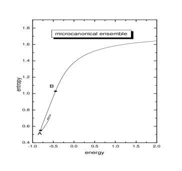
Figure 5: Entropy versus energy: Equilibrium configurations exit only for $\epsilon>\epsilon_{A}$.

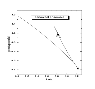
Figure 6: Planck potential versus inverse temperature: the canonical ensemble access only to those equilibrium stages with $\beta<\beta_{B}$ ($\epsilon>\epsilon_{B}$).

The Gibbs’ argument, the equilibrium of a subsystem with a thermal bath, is non applicable to this situation because of no reasonable thermal bath exits for the astrophysical systems.Therefore, the isothermal catastrophe is not a phenomenon with physical relevance since it can be never obtained in nature: the consideration of a thermal bath in the astrophysical system is outside of context. A different significance possesses the gravothermal catastrophe. The gravitational collapse is the main engine of structuration in astrophysics and it concerns almost all scales of the universe: the formation of planetesimals in the solar nebula, the formation of stars, the fractal nature of the interstellar medium, the evolution of globular clusters and galaxies and the formation of galactic clusters in cosmology chava3 .

Let us now carry out a comparative study between the isothermal model and this alternative onel. As already mentioned, the only difference between these approaches relies on the regularization prescription of the long-range singularity of the selfgravitating gas: the isothermal model avoids the particles evaporation by using a rigid container, while the present model takes into account the effect of this evaporation by truncating the kinetic energy distribution function. This study is carried out by considering a spherical container in the isothermal model with a linear dimension $R=R_{tidal}$.

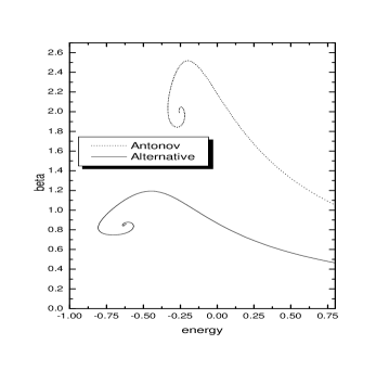
Figure 7: The caloric curves.The figure shows the comparison between the two models.

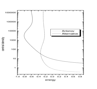
Figure 8: The central density versus energy. The central density is much greater in this alternative version of the Antonov problem.

Figure (7) shows the caloric curves of these models. In spite of the qualitative similarity of these dependences, the alternative model is able to describe an additional energetic range: from $-0.806$ to $-0.335$; but the isothermal model describes equilibrium configurations belonging to the interval $1.193<\beta<2.518$, which are cooler than the ones described by using the first model..

A second difference is evidenced in regard to the central density versus energy dependence, which is shown in the figure (8). The central density at the critical energy of the gravitational collapse is much greater in the alternative model than the isothermal one, and this qualitative relationship seems to be applicable to the whole energetic range.

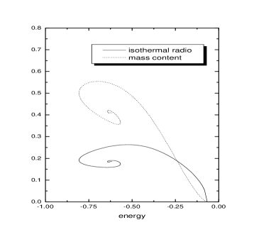
Figure 9: Isothermal core radio and its mass content in the alternative model.

The figure (9) shows two interesting observables: the radio in which the system exhibits an isothermic behavior, $R_{i.c}$, and the mass content enclosed inside, $M_{i.c}$. This quantities characterizes the size and the mass of the isothermal core. The reader may observe that the isothermal core contains at the critical energy of the gravitational collapse, the half of the system total mass inside the $\sim 1\%$  of the system volume. On the other hand, it is interesting to note that this isothermal core disappears at $\epsilon^{\ast}\simeq-0.066$.

The quantitative differences in the thermodynamical description between these models seem to be explained by the following reasonings. Most of the energy contribution to the total energy comes from the isothermal core. The contribution of the gravitational potential energy is dominant in the core due to the high mass concentration enclosed inside this region, where moreover, the Newtonian potential exhibits its highest values. Outside the isothermal core, the kinectic energy contribution decreases considerably as consequence of the deviation from the isothermal character of the microscopic particles distribution function due to the evaporation.

These arguments can be rephrased as follows: in the isothermal region, where $-0.806<\epsilon<-0.066$, the present model behaves as an isothermal model with a characteristic size equal to the size of the isothermal core. Since the relevant canonical variables in the isothermal model is $\eta=\beta GM/R$ antonov ; chava3 , a rough estimation of the maximal value $\beta_{\max}=\beta_{B}$ in which the isothermal collapse takes places is given by:

$$\beta_{B}\approx\frac{R_{i.c}}{M_{i.c}}\beta_{\max}^{isoth.}.$$ (62)

By using the characteristics values $R_{i.c}\approx 0.2$, $M_{i.c}\approx 0.5$, and $\beta_{\max}^{isoth.}\approx 2.5$ (obtained from the isothermal model), the formula (62) gives a fairly good estimation of $\beta_{B}\approx 1$ ($\beta_{B}=1.193$).

The main difference between these model is in regard to the character of the equilibrium profiles in the high energy region with $\epsilon>0$. As already discussed, the isothermal core has disappear in this energetic region and the equilibrium configurations of the system are essentially polytropic, while the isothermal model leads to a uniform distribution of the particles throughout the volume of the rigid container.

In this case, the structure equations (47) become in a quasi-polytropic model:

$$\Delta\Phi =-4\pi\exp\left(\Psi\right)\frac{4}{3\sqrt{\pi}}\Phi^{\frac{3}{2}},\text{ \ }$$

$$\Delta\Psi =-4\pi\exp\left(\Psi\right)\frac{2}{\sqrt{\pi}}\Phi^{\frac{1}{2}},$$ (63)

which exhibits the same fractal characteristics of a polytropic model with polytropic index $\gamma=\frac{5}{3}$. This polytropic index characterizes an adiabatic process of the ideal gas of particles, which is in our case the evaporation of the system in the vacuum. However, this equation system is not equivalent to the polytropic model due to the presence of the driving function $C$. This purely polytropic profile is obtained by disregarding the second equation and setting $\Psi\equiv 0$ in the first one.

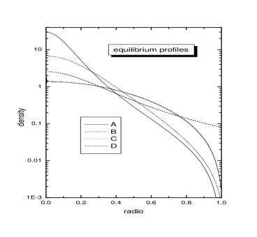
Figure 10: Comparison among the equilibrium profiles: A) Alternative model with an isothermal core, B) Isothermal profile, C) Alternative model with a quasi-polytropic profile, and D) Purely polytropic profile.

Let us finalize our discussion by carrying out a comparative study among the equilibrium profiles obtained from the alternative model with the well-known isothermal and polytropic profiles. These equilibrium profiles are shown in the figure (10). Equilibrium profiles A and C were obtained from the alternative model: profile A corresponds to an equilibrium configuration possessing an isothermal core, while C is a quasi-polytropic equilibrium profile. Profiles B and D correspond respectively to an isothermal and polytropic configurations. The reader can note that the alternative model profiles differ essentially in regard to the existence of the isothermal core, since no qualitative differences are evidenced in the halo structure. On the other hand, these results suggest that a system undergoing an evaporation process concentrates their particles in the inner regions more than what the isothermal or the polytropic models predict.

V Conclusions

As already shown in the present paper, the consideration of the energetic prescription (1) leads to an alternative version of the Antonov problem. This model, besides of exhibiting the main features of the isothermal model: the gravitational collapse and the energetic region with a negative specific heat, has the advantage that the system size naturally appears as consequence of the particles evaporation. There is no need of enclosing the system in a rigid container in order to avoid long-range singularity of the Newtonian potential because this regularization procedure is sufficient to access to finite equilibrium configurations.

It is remarkable that the present approach unifies the well-known isothermal and polytropic equilibrium profiles. As already mentioned, the equilibrium profiles derived from this alternative model differ essentially in regard to the existence of the isothermal core, since no qualitative differences are evidenced in the halo structure. The comparative study of the equilibrium $\rho$ profiles suggests that a system undergoing an evaporation process concentrates the particles in the inner regions more than what predict by the isothermal or the polytropic models.

There are many open questions in the study of this model system by using this kind of regularization scheme, as example, the dynamical aspects: Which is the influence of the particles evaporation in the system dynamical evolution? and how could it be performed this dynamical description by preserving this energetic prescription? Further studies should clarify these questions. The present study is carried out by considering that the evaporation rate is small enough in order to ensure that the system reaches a quasistationary state. This assumption is satisfied by the globular clusters, since the relaxation time $t_{relax}$ in them differs considerable from the evapotation time $t_{evap}$, $t_{relaz}\ll t_{evap}$ (see in ref.berna ). The dynamical approch could be developed by considering that the system evolutes slowly throughout these quasistationary states.

References

- (1) T. Padmanabhan, Phys. Rep. 188 , 285 (1990).
- (2) M. Kiessling, J. Stat. Phys. 55 , 203 (1989).
- (3) D. Ruelle, Helv. phys. Acta 36 , 183 (1963). M.E. Fisher, Archive for Rational Mechanics and Analysis 17 , 377 (1964).
- (4) J. van der Linden, Physica 32 , 642 (1966); ibid 38 , 173 (1968); J. van der Linden and P. Mazur, ibid 36 , 491 (1967).
- (5) V.A. Antonov, Vest. leningr. gos. Univ. 7 , 135 (1962).
- (6) D. Lynden-Bell and R.Wood, 1968, MNRAS, 138, 495. D. Lynden-Bell. Mon. Not. R. Astron. Soc. 136 101 (1967).
- (7) D. Lynden-Bell and R. Wood, Mon. Not. R. Ast. Soc. 138 , 495 (1968).
- (8) W. Thirring, Z. Phys. 235 , 339 (1970).
- (9) E.V. Votyakov, H.I. Hidmi, A. De Martino, and D.H.E. Gross, Phys. Rev. Lett. 89 (2002) 031101; e-print (2002) [cond-mat/0202140].
- (10) H.J. de Vega and N. Sanchez, Phys. Lett. B 490 , 180 (2000); Nucl. Phys. B 625 , 409 (2002); ibid, 460.
- (11) J. Binney and s. Tremaine, Galactic Dynamics (Princeton Series in Astrophysics, Pricenton, NJ, 1987).
- (12) P. H. Chavanis, Phys. Rev. E 65 , 056123 (2002); P.H. Chavanis and I. Ispolatov, Phys. Rev. E 66 , 036109 (2002).
- (13) P. H. Chavanis, C. Rosier and C. Sire, preprint ( 2001) [cond-mat/0107345].
- (14) M. J. Benacquista, Relativistic Binaries in Globular Clusters, e-print (2002) [www.livingreviews.org /Articles /Volume5 /2002-2benacquista].