Conductivity of Paired Composite Fermions

Abstract

We develop a phenomenological description of the $\nu=5/2$ quantum Hall state in which the Halperin-Lee-Read theory of the half-filled Landau level is combined with a $p$-wave pairing interaction between composite fermions (CFs). The electromagnetic response functions for the resulting mean-field superconducting state of the CFs are calculated and used in an RPA calculation of the $q$ and $\omega$ dependent longitudinal conductivity of the physical electrons, a quantity which can be measured experimentally.

The $\nu=5/2$ fractional quantum Hall state remains one of the most interesting phenomena in two dimensional electron physics[1]. Since its experimental discovery over a decade ago[2], the nature of this state has been a topic of debate. Evidence from exact diagonalizations of small systems[3] now seems to point towards the 5/2 state being properly described as a spin-polarized Moore-Read Pfaffian state[4], a state which can be viewed as a chiral $p$-wave superconductor[4, 5] of composite fermions (CFs) [6]. Among other interesting ramifications, the Moore-Read state should theoretically exhibit excitations with exotic nonabelian statistics[4] — something never before observed in nature.

Although there is a reasonably strong theoretical case that the $\nu=5/2$ FQHE state is, in fact, a Moore-Read state, the question remains, how can one test this hypothesis experimentally? While several experiments seem to be at least consistent with the 5/2 state being a Moore-Read state[7, 3], we are still in need of a smoking gun. The analogy with superconductivity makes one think of how the classic experimental hallmarks of BCS-superconductivity[8] theory might be translated into the fractional quantum Hall regime. For example, in traditional superconductors, many measurable response functions display “coherence peaks” below the critical temperature which are extremely good evidence of BCS superconductivity. We would like to ask whether such a phenomena should exist for the Moore-Read state (or, for that matter, if any other clear signature could be seen in measurable response functions.) To address this question, we have developed a phenomenological description of the FQHE state in which the Halperin-Lee-Read(HLR) [9] theory of the half-filled Landau level is combined with a $p$-wave pairing interaction between CFs. Within this theory we are able to predict various response functions of the Moore-Read state which may be measured experimentally. Recalling that surface acoustic waves (SAW) experiments[6] were particularly powerful in experimentally demonstrating the existence of CFs, we will be particularly interested in the SAW signatures of the Moore-Read state.

In the HLR theory[9], each electron in modeled as a fermion bound to two quanta of “Chern-Simons” flux, the fermion plus flux being called a CF. For the 5/2 state, 4/5 of the electrons are required to fill the lowest two (essentially inert) Landau bands and the remaining (1/5) valence electrons are transformed to CFs. At the mean field level, the external field precisely cancels the bound flux and we model the valence electrons as free fermions in zero effective magnetic field. There is some indication that under certain conditions the residual interaction between the CFs can create a pairing instability[5, 10]. To represent this physics, we add a pairing interaction between the CFs by hand. We thus use a model Hamiltonian for the CFs of the standard BCS form ($\hbar=c=1$ throughout),

$$H=\!\!\sum_{{\bf k}}\xi_{\bf k}c^{\dagger}_{{\bf k}}c_{{\bf k}}+\!\frac{1}{2}\!\sum_{{\bf k},{\bf k}^{\prime},{\bf q}}\!\!V_{{\bf k}{\bf k}^{\prime}}c^{\dagger}_{{\bf k}+\frac{\bf q}{2}}c^{\dagger}_{-{\bf k}+\frac{{\bf q}}{2}}c^{\phantom{\dagger}}_{-{\bf k}^{\prime}+\frac{\bf q}{2}}c^{\phantom{\dagger}}_{{{{\bf k}}^{\prime}+\frac{\bf q}{2}}},$$ (1)

where $c^{\dagger}$ is the CF creation operator, $\xi_{k}=k^{2}/(2m)-\mu$ and $m$ is CF effective mass which may be much larger than the underlying electron mass. (Note that the ad-hoc mass renormalization will cause problems at the cyclotron energy scale but is expected to be reasonable at lower energies[9, 11].) In the spirit of Ref [9] we will calculate the CF response of the Hamiltonian (1) then transform this result (See Eq. 22 below) to determine the physical electron response.

In Eq. 1 the pairing interaction is taken to be of chiral $p$-wave form $V_{{\bf k}{\bf k}^{\prime}}=-Ve^{-i\theta_{\bf k}}e^{i\theta_{{\bf k}^{\prime}}}$ where $\theta_{\bf k}$ is the angle of ${\bf k}$ on the Fermi surface. Note that this interaction is not time-reversal symmetric — it is only attractive in the $l=+1$ channel, not the $l=-1$ channel. Such an asymmetry is expected because, although the CFs see zero average magnetic field at the mean-field level, their residual interactions are not time-reversal symmetric.

If we define the gap function to be

$$\Delta_{\bf q}\equiv V\sum_{{\bf k}^{\prime}}\langle c_{-{\bf k}^{\prime}+\frac{{\bf q}}{2}}c_{{\bf k}^{\prime}+\frac{{\bf q}}{2}}\rangle e^{i\theta_{{\bf k}^{\prime}}},$$ (2)

the BCS mean-field Hamiltonian can be written in pseudospin notation as

$$H_{MF}=\frac{1}{2}\sum_{\bf k}\Psi_{\bf k}^{\dagger}\left(\xi_{\bf k}\tau_{z}-\Delta(\cos\theta_{\bf k}\tau_{x}+\sin\theta_{\bf k}\tau_{y})\right)\Psi_{\bf k},$$ (3)

where $\tau_{x},\tau_{y},\tau_{z}$ are the usual Pauli spin matrices, $\Psi^{\dagger}_{\bf k}=(c^{\dagger}_{\bf k},~{}~{}c_{-{\bf k}})$ and $\Delta=|\Delta_{{\bf q}=0}|$ is the temperature dependent energy gap found by solving the usual BCS gap equation. It is important to note that the restriction of $\Delta_{{\bf q}}$ to its zero wavevector component explicitly breaks gauge invariance. We will fix this problem below.

We now add a perturbation Hamiltonian to the above $H_{MF}$ given by

$$H^{\prime}=\sum_{{\bf q}}\left[{a_{0}}_{\bf q}{j_{0}}_{-{\bf q}}+{a_{1}}_{\bf q}{j_{1}}_{-{\bf q}}+{a_{b}}_{\bf q}{{j_{b}}_{-{\bf q}}}\right],$$ (4)

where

$$\!\!\!({j_{0}}_{\bf q},{j_{1}}_{\bf q})=\frac{1}{2}e\sum_{{\bf k}}\Psi^{\dagger}_{{{\bf k}+{\bf q}/2}}(\tau_{z},\frac{k_{\perp}}{m}\tau_{0})\Psi_{{\bf k}-{\bf q}/2},$$ (5)

$${j_{b}}_{\bf q} = \frac{1}{2}\sum_{k}\Psi_{{\bf k}+{\bf q}/2}^{\dagger}(-\cos\theta_{\bf k}\tau_{y}+\sin\theta_{\bf k}\tau_{x})\Psi_{{\bf k}-{\bf q}/2}.$$ (6)

The first two terms in $H^{\prime}$ are the coupling of the scalar potential ${a_{0}}_{\bf q}$ to the density ${j_{0}}_{\bf q}$ and the transverse vector potential ${a_{1}}_{\bf q}$ to the transverse paramagnetic current ${j_{1}}_{\bf q}$(for simplicity we work in Coulomb gauge here so the longitudinal vector potential is zero). The third term in $H^{\prime}$ is the coupling of CFs to the phase fluctuations of the order parameter, described by ${a_{b}}_{\bf q}=(\Delta_{\bf q}-\Delta_{-{\bf q}}^{*})/(2i)$ which will be self-consistently calculated. Such a self-consistent treatment of phase fluctuations is a standard method[12] that enables one to calculate gauge invariant responses to external perturbations despite the fact that $H_{MF}$ is not gauge invariant by itself. Magnitude fluctuations are neglected since they can be shown to decouple due to approximate particle-hole symmetry at the Fermi surface [13].

We define the response functions $Q_{ij}$ for the mean-field Hamiltonian $H_{MF}$ by

$$j_{i}({\bf q},\omega) = Q_{ij}({\bf q},\omega)a_{j}({\bf q},\omega),$$ (7)

where the indices $i$ and $j$ can be $0$, $1$ or $b$. Here $j_{i}({\bf q},\omega)$ is the fourier transform of the time-dependent expectation value of ${j_{i}}_{\bf q}+\delta_{i1}(n/m){a_{1}}_{\bf q}$ and thus includes the diamagnetic contribution to the transverse current.

When the constraint, following from (2), that ${a_{b}}_{\bf q}=V\langle{j_{b}}_{\bf q}\rangle$ is included, the standard RPA analysis [12] can be used to obtain the gauge invariant CF electromagnetic response functions $K_{\mu\nu}$ defined by

$$j_{\mu}({\bf q},\omega)=K_{\mu\nu}({\bf q},\omega)a_{\nu}({\bf q},\omega),$$ (8)

where the indices $\mu$ and $\nu$ can now be $0$ or $1$. We obtain

$$K_{\mu\nu}=Q_{\mu\nu}-Q_{\mu b}Q_{b\nu}/(Q_{bb}-1/V),$$ (9)

where the second term on the right hand side corresponds to the usual vertex corrections required for a conserving approximation.

Following Mattis and Bardeen [14] (see also [15]), in the extreme anomalous limit $v_{F}q\gg{\rm Max}[\omega,\Delta]$ the expressions for these response functions can be simplified substantially. We obtain

$$Q_{00}({\bf q},\omega) = -\frac{m^{2}}{4\pi^{2}}F_{0}(q)\Omega(1,-\cos\theta_{q},\omega)-\frac{m}{2\pi},$$ (10)

$$Q_{10}({\bf q},\omega) = i\sin\theta_{\bf q}\frac{m}{4\pi^{2}}F_{1}(q)\Omega(0,1,\omega),$$ (11)

$$Q_{11}({\bf q},\omega) = \frac{1}{4\pi^{2}}F_{2}(q)\Omega(1,\cos\theta_{q},\omega)-\frac{q^{2}}{24\pi m},$$ (12)

$$Q_{b0}({\bf q},\omega) = i\frac{m^{2}}{4\pi^{2}}F_{0}(q)\frac{\omega}{\Delta}\cos\frac{\theta_{\bf q}}{2}\Omega(0,1,\omega),$$ (13)

$$Q_{b1}({\bf q},\omega) = \frac{m}{4\pi^{2}}F_{1}(q)\frac{\omega}{\Delta}\sin\frac{\theta_{\bf q}}{2}\Omega(0,1,\omega),$$ (14)

$$Q_{bb}({\bf q},\omega) = \frac{m^{2}}{4\pi^{2}}F_{0}(q)\Omega(1,-1,\omega)+\Lambda({\bf q})+\frac{1}{V},$$ (15)

where $\theta_{q}$ is the angle between the vectors ${{\bf k}+{\bf q}/2}$ and ${{\bf k}-{\bf q}/2}$ when constrained to the Fermi surface, and $Q_{0b}({\bf q},\omega)=-Q_{b0}({\bf q},\omega)$, $Q_{b1}({\bf q},\omega)=Q_{1b}({\bf q},\omega)$, $Q_{10}({\bf q},\omega)=Q_{01}({\bf q},\omega)$. In these equations,

$$F_{\alpha}(q)=(2k_{f}^{\alpha-1}/q)\left[1-q^{2}/(2k_{f})^{2}\right]^{(\alpha-1)/2},$$ (16)

and $\Omega(\omega)=\Omega_{1}(\omega)+i\Omega_{2}(\omega)$ with

$$\Omega_{1}(r,s,\omega) = \pi\int_{{\rm max}[\Delta-\omega,-\Delta]}^{\Delta}\left(1-2f(E+\omega)\right)\frac{sE(E+\omega)+r\Delta^{2}}{[\Delta^{2}-E^{2}]^{1/2}[(E+\omega)^{2}-\Delta^{2}]^{1/2}}dE,$$ (17)

$$\Omega_{2}(r,s,\omega) = -2\pi\int_{\Delta}^{\infty}\left(f(E)-f(E+\omega)\right)\frac{sE(E+\omega)+r\Delta^{2}}{[E^{2}-\Delta^{2}]^{1/2}[(E+\omega)^{2}-\Delta^{2}]^{1/2}}dE$$ (20)

$$~{}~{}~{}~{}~{}~{}~{}-\pi\int_{\Delta-\omega}^{-\Delta}\left(1-2f(E+\omega)\right)\frac{sE(E+\omega)+r\Delta^{2}}{[E^{2}-\Delta^{2}]^{1/2}[(E+\omega)^{2}-\Delta^{2}]^{1/2}}dE,$$

$$\Lambda({\bf q}) = \int\frac{d^{2}k}{(2\pi)^{2}}\left(\frac{1-f(\xi_{{{\bf k}-{\bf q}/2}})-f(\xi_{{{\bf k}+{\bf q}/2}})}{\xi_{{{\bf k}-{\bf q}/2}}+\xi_{{{\bf k}+{\bf q}/2}}}-\frac{1-2f(E_{\bf k})}{2E_{\bf k}}\right),$$ (21)

where $E_{\bf k}=\sqrt{\xi_{\bf k}^{2}+|\Delta|^{2}}$ and $f$ is the Fermi function. The one dimensional integrals for $\Omega(\omega)$ are easily evaluated numerically. In the extreme anomalous limit $\Lambda({\bf q})\simeq-(m/(2\pi))\log(v_{F}q/(2\Delta(0))$ is large and the vertex corrections to the Coulomb gauge are small.

Note that this mean-field treatment gives a finite temperature phase transition. It should be emphasized that this is an artifact of our calculation. Vortices in a Chern-Simons “superfluid” cost a finite amount of energy to create and interact only via short-range interactions. As a result there is no finite temperature Kosterlitz-Thouless transition and fluctuations will push $T_{c}$ to zero. We assume here that including these fluctuations will primarily have the effect of smoothing the finite temperature transition into a crossover, but the qualitative features of our results will remain.

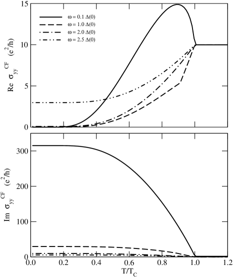
FIG. 1.: Real and Imaginary parts of the transverse conductivity of composite fermions, $\sigma_{yy}^{CF}$, in a $p$-wave “superconducting” state as a function of temperature for $\omega/\Delta(0)=$ 0.1, 1.0, 2.0 and 2.5. For low frequencies, $\omega\ \vbox{\hbox{$<$}\offinterlineskip\hbox{$\sim$}}\ 0.2\Delta$, ${\rm Re}\ \sigma_{yy}^{CF}$ shows a Hebel-Slichter coherence peak and ${\rm Im}\ \sigma_{yy}^{CF}$ shows a strongly enhanced diamagnetic response. Results are for $\Delta(0)=0.01E_{F}$ and $q=0.1k_{F}$.

To fix the parameters of our model, in all of what follows we take $\Delta(0)/E_{F}=0.01$. This is consistent with $k_{f}=(4\pi n/5)^{1/2}\sim 10^{8}$ m^-1, $\Delta(0)\sim 0.1$ K, and a CF effective mass $m\sim 10m_{b}$ where $m_{b}$ is the electronic band mass.

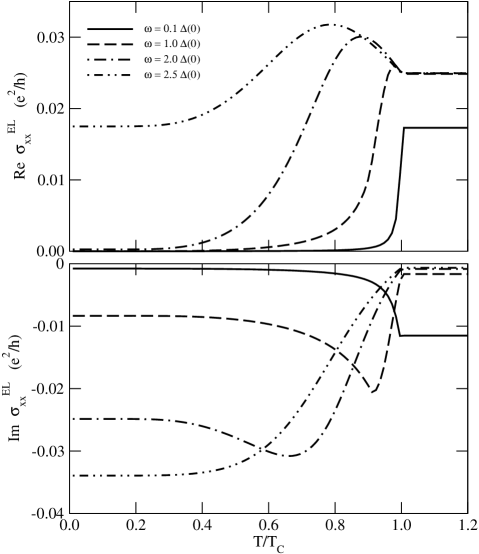
FIG. 2.: Real and imaginary parts of the longitudinal conductivity of electrons, $\sigma_{xx}^{EL}$, for the same parameters as Fig. 1. In this regime, $\sigma_{xx}^{EL}\propto 1/\sigma_{yy}^{CF}$, and because of the strongly enhanced ${\rm Im}\ \sigma_{yy}^{CF}$ for $\omega\ \vbox{\hbox{$<$}\offinterlineskip\hbox{$\sim$}}\ 0.2\Delta$ (see Fig. 1) there is no sign of the Hebel-Slichter peak in $\sigma_{xx}^{EL}$.

Coherence effects are most clearly seen in the $q$ and $\omega$ dependent conductivity. Figure 1 shows the transverse conductivity $\sigma^{CF}_{yy}=e^{2}K_{11}/i\omega$ for CFs as a function of temperature for $q=0.1k_{F}$. For low frequencies, $\omega\ \vbox{\hbox{$<$}\offinterlineskip\hbox{$\sim$}}\ 0.2\Delta(0)$, ${\rm Re}\ \sigma^{CF}_{yy}$ shows a Hebel-Slichter coherence peak just below $T_{c}$. This peak appears because for small $q$ the $p$-wave nature of the pairing is irrelevant and the coherence factors which determine electromagnetic absorption are Type II, the same coherence factors which govern the temperature dependence of the NMR relaxation time $1/T_{1}$ in conventional superconductors. For the same low frequencies ${\rm Im}\ \sigma^{CF}_{yy}$ increases dramatically below $T_{c}$, reflecting the large increase in ${\rm Re}\ K_{11}(q,\omega)$ due to the enhanced CF diamagnetic response in the paired state. Note that the kink clearly visible in ${\rm Re}\ \sigma^{CF}_{yy}$ for $\omega=\Delta(0)$ occurs when the threshold condition $\omega=2\Delta(T)$ is satisfied.

It is natural to ask if a similar coherence peak is observable in the 5/2 state. To address this we calculate the experimentally measurable electronic longitudinal conductivity, $\sigma_{xx}^{EL}$, following HLR using the Chern-Simons RPA. The only modification to the HLR result is due to the off-diagonal part of the mean-field CF response function – a consequence of the chiral nature of the $p$-wave state. The resulting expression for the conductivity is

$$\sigma^{EL}_{xx}=\frac{ie^{2}\omega K_{00}/q^{2}}{1+\frac{4\pi i\tilde{\phi}}{q}K_{10}+\frac{(2\pi\tilde{\phi})^{2}}{q^{2}}(K_{00}K_{11}-K_{10}^{2})},$$ (22)

where $\tilde{\phi}=2$ is the number of flux quanta attached to each CF. Just as in the HLR case, in the limit of small $q$ this expression is dominated by $K_{11}$ and to a good approximation $\sigma^{EL}_{xx}\simeq(e^{2}/(2\pi\tilde{\phi})^{2})i\omega K_{11}^{-1}=(e^{2}/(2\pi\tilde{\phi}))^{2}/\sigma_{yy}^{CF}$.

Figure 2 shows the electronic longitudinal conductivity for the same parameters as Fig. 1. The main observation is that there is no sign of the Hebel-Slichter peak at low frequencies. This is because of the rapid increase in ${\rm Im}\ \sigma_{yy}^{CF}$ below $T_{c}$ discussed above. This rapid increase suppresses $\sigma_{xx}^{EL}$ below $T_{c}$, masking the relatively small Hebel-Slichter peak. We note that if one could measure the real and imaginary parts of $\sigma_{xx}^{EL}$ to sufficient accuracy to carry out the inversion to obtain $\sigma_{yy}^{CF}$ one could in principle observe the Hebel-Slichter peak, although in practice such accuracy would be very difficult to achieve.

Note that for $\omega\mathrel{\hbox to0.0pt{\lower 4.0pt\hbox{\hskip 1.0pt$\sim$}\hss}\raise 1.0pt\hbox{$>$}}\Delta$ a peak in $\mbox{Re}\ \sigma_{xx}^{EL}$ does appear below $T_{C}$. We emphasize that this is not a coherence peak but rather a consequence of the fact that the absolute magnitude of $\sigma_{yy}^{CF}$ decreases below $T_{c}$ for these frequencies.

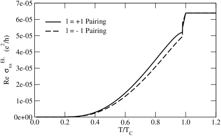
FIG. 3.: Longitudinal conductivity of electrons for $\omega=0.5\Delta(0)$ and $q=0.75k_{F}$. Results are shown for pairing angular momentum parallel and antiparallel to the applied field. The small difference indicates the $p$-wave nature of the pairing is difficult to observe in $\sigma^{EL}_{xx}$, even at large wavevectors. Results are for $\Delta(0)=0.01E_{F}$.

All the results shown to this point are for $q\ll k_{F}$. This is the regime for which the HLR theory is expected to be qualitatively correct. It must be emphasized that in this limit the $p$-wave nature of the pairing is irrelevant and the results would be the same for $s$-wave (up to factors of 2 from the fact that we need two spin states), or any $l$-wave, CF superconductors. The $p$-wave nature of the pairing only becomes relevant when $q$ is large enough to span parts of the Fermi surface where the phase of the order parameter is significantly different.

A measure of the relevance of the $p$-wave pairing can be seen by comparing results for which the applied magnetic field is parallel and antiparallel to the pair angular momentum. This corresponds to changing the sign of $\tilde{\phi}$ in (22). For $q\ll k_{F}$, including all results presented above, there is no measurable difference for these two cases. For $q\sim k_{F}$, a difference in $\sigma^{EL}_{xx}$ appears, but it is small. A typical result is shown in Fig. 3.

To summarize, we have developed a phenomenological model of the 5/2 state by adding a chiral $p$-wave pairing interaction between CFs by hand. The electromagnetic CF response functions for this model were then calculated, including self-consistent fluctuations of the order parameter to ensure gauge invariance. For small $q$ the CF transverse conductivity exhibits a Hebel-Slichter peak, but this peak is not easily observable in measurements of the electronic longitudinal conductivity. Although we have focused on the question of whether clear signatures of superconductivity can be seen in SAW measurements, similar calculations can give predicitions for other electromagnetic response experiments, such as microwave conductivity and resonant Raman scattering[16]. Furthermore, the methods described here can be more generally applied to analyze a variety of other paired CF states — including the Haldane-Rezayi[17] state and several proposed paired bilayer states[18].

The authors thank Kun Yang for useful discussions. KCF and NEB acknowledge support from US DOE Grant No. DE-FG02-97ER45639.

REFERENCES

- [1] For a review on the status of the state, see N. Read, Physica B 298 121, 2001; cond-mat/0011338.
- [2] R.L. Willett et al., Phys. Rev. Lett. 59, 1776 (1987).
- [3] R. Morf, Phys. Rev. Lett. 80, 1505 (1998); E.H. Rezayi and F.D.M. Haldane, Phys. Rev. Lett. 84, 4685 (2000).
- [4] G. Moore and N. Read, Nucl. Phys. B 360, 362 (1991).
- [5] M. Greiter, X.G. Wen, and F. Wilczek, Phys. Rev. Lett. 66, 3205 (1991); Nucl. Phys. B 374, 567 (1992).
- [6] For a review of CFs see “Composite Fermions”, ed O. Heinonen, World Scientific, 1998; and therein.
- [7] R. L. Willett, K. W. West, and L. N. Pfeiffer Phys. Rev. Lett. 88, 066801 (2002); W. Pan et al., Phys. Rev. Lett. 83, 3530 (1999); J. P. Eisenstein, et al., Phys. Rev. Lett. 61, 997 (1988).
- [8] See for example, “Theory of Superconductivity”, J. R. Schrieffer, Addison Wesley, 1964.
- [9] B.I. Halperin, P.A. Lee, and N. Read, Phys. Rev. B 47, 7312 (1993).
- [10] N. E. Bonesteel Phys. Rev. Lett. 82, 984-987 (1999)
- [11] S. H. Simon and B. I. Halperin, Phys. Rev. B 48, 17368 (1993).
- [12] P.W. Anderson, Phys. Rev. 112, 1900 (1958); G. Rickayzen, Phys. Rev. 115, 795 (1959).
- [13] I.O. Kulik, O. Entin-Wohlman and R. Orbach, J. Low Temp. Phys. 43, 591 (1981).
- [14] D.C. Mattis and J. Bardeen, Phys. Rev. 111, 412 (1958)
- [15] M.U. Ubbens and P.A. Lee, Phys. Rev. B 49, 6853 (1994).
- [16] See, for example, “Perspectives on Quantum Hall Effects”, S. Das Sarma and A. Pinczuk, eds., Wiley, 1997.
- [17] F. D. M. Haldane and E. H. Rezayi, Phys. Rev. Lett. 60, 956 (1988).
- [18] N.E. Bonesteel, I.A. McDonald and C. Nayak, Phys. Rev. Lett. 77, 3009 (1996); Y.B. Kim et al., Phys. Rev. B, 205315 (2001).