Stable Equilibrium Based on Lévy Statistics: A Linear Boltzmann Equation Approach

Abstract

To obtain further insight on possible power law generalizations of Boltzmann equilibrium concepts, a stochastic collision model is investigated. We consider the dynamics of a tracer particle of mass $M$, undergoing elastic collisions with ideal gas particles of mass $m$, in the Rayleigh limit $m<<M$. The probability density function (PDF) of the gas particle velocity is $f\left(\tilde{v}_{m}\right)$. Assuming a uniform collision rate and molecular chaos, we obtain the equilibrium distribution for the velocity of the tracer particle $W_{eq}(V_{M})$. Depending on asymptotic properties of $f\left(\tilde{v}_{m}\right)$ we find that $W_{eq}(V_{M})$ is either the Maxwell velocity distribution or a Lévy distribution. In particular our results yield a generalized Maxwell distribution based on Lévy statistics using two approaches. In the first a thermodynamic argument is used, imposing on the dynamics the condition that equilibrium properties of the heavy tracer particle be independent of the coupling $\epsilon=m/M$ to the gas particles, similar to what is found for a Brownian particle in a fluid. This approach leads to a generalized temperature concept. In the second approach it is assumed that bath particles velocity PDF scales with an energy scale, i.e. the (nearly) ordinary temperature, as found in standard statistical mechanics. The two approaches yield different types of Lévy equilibrium which merge into a unique solution only for the Maxwell–Boltzmann case. Thus, relation between thermodynamics and statistical mechanics becomes non-trivial for the power law case. Finally, the relation of the kinetic model to fractional Fokker–Planck equations is discussed.

I Introduction

Khintchine Khin revealed the deep relation between the Gaussian central limit theorem and classical Boltzmann– Gibbs statistics. From a simple stochastic point of view, we may see this relation by considering the velocity of a Brownian particle. The most basic phenomenological dynamical description of Brownian motion, is in terms of the Langevin equation $\dot{V}_{M}=-\gamma V_{M}+\eta(t)$, where $\eta(t)$ is a Gaussian white noise term. Usually the assumption of Gaussian noise is imposed on the Langevin equation to obtain a Maxwellian velocity distribution describing the equilibrium of the Brownian particle. We may reverse our thinking of the problem, the Gaussian noise is naturally expected based on central limit theorem arguments, and the latter leads to Maxwell’s equilibrium. Similar arguments hold for a Brownian particle in an external time independent binding force field, the Maxwell–Boltzmann equilibrium is obtained in the long time limit only if the noise term is Gaussian. Yet another case where the relation between Gaussian statistics and statistical mechanics is seen is Feynman’s Gaussian path integral formulation of statistical mechanics.

However, Gaussian central limit theorem is non unique. Lévy, and Khintchine Feller have generalized the Gaussian central limit theorem, to the case of summation of independent, identically distributed random variables described by long tailed distributions. In this case Lévy distributions replace the Gaussian in generalized limit theorems. Hence it is natural to ask Montroll ; Grigolini ; Chechkin ; Zannette if a Lévy based statistical mechanics exist? And if so what is its physical domain and its relation to thermodynamics. This type of questions are timely due to the interest in generalizations of statistical mechanics Abe ; Long ; CohenEDG ; Gallavotti , mainly non-extensive statistical mechanics due to Tsallis Tsallis . While Lévy statistics is used in many applications Bouch1 ; review ; Cohen ; Zaslavsky ; Barkai1 ; Barkai2 ; Barkai3 , its possible relation to generalized equilibrium statistical mechanics is still unclear.

As well known, Boltzmann used a kinetic approach for a dilute gas of particles to derive Maxwell’s velocity distribution, his starting point being his non-linear equation (see conditions in Cercignani ). Thus, the kinetic approach can be used as a tool to derive equilibrium, starting from non-equilibrium dynamics. Ernst Ernst , shows how the Maxwell equilibrium is obtained from several stochastic collision models. More recently, Chernov and Lebowitz CL investigated numerically a gas $+$ heavy piston system, showing that the gas particle velocity distribution approaches a Maxwellian distribution, starting from a non-Maxwellian initial condition. Thus, the Maxwell equilibrium transcends details of individual kinetic models. It is important to note that in these works, important boundary and initial conditions are imposed on the dynamics Cercignani ; Ernst ; CL ; Lar . For example, the second moment of the velocity of the particles is supposed to be finite, Eqs. 1.7 and 2.10 in Ernst . A possible domain of power law generalizations of Maxwell’s equilibrium, are the cases where one does not impose ‘finite variance’ initial and/or boundary conditions.

In this manuscript we will consider a simple kinetic approach to obtain a generalization of Maxwell’s velocity distribution. Briefly we consider a one dimensional tracer particle of mass $M$ randomly colliding with gas particles of mass $m<<M$. Two main assumptions are used: (i) molecular chaos holds, implying lack of correlations in the collision process (Stoszzahlansantz), and (ii) rate of collisions is independent of the energy of the colliding particles. Let the probability density function (PDF) of velocity of the gas particles be $f\left(\tilde{v}_{m}\right)$. If $f\left(\tilde{v}_{m}\right)$ is Maxwellian, the model describes Brownian type of motion for the heavy particle, the equilibrium being the Maxwell distribution Kampen ; Opp ; BF . Since our aim is to investigate generalized equilibrium, we do not impose the standard condition of Maxwellian velocity distribution for the bath particles. Our aim is to show, under general conditions, that the equilibrium PDF of the tracer particle $W(V_{M})$ is stable. Stable means here that large classes of velocity distributions for bath particles $f(\tilde{v}_{m})$ will yield a unique type of equilibrium for the tracer particle $W_{eq}(V_{M})$. Namely the equilibrium velocity distribution transcends the details of precise shape of $f(\tilde{v}_{m})$. One of those stable velocity distributions will turn out to be Maxwell’s velocity distribution.

To obtain an equilibrium we use two approaches. The first we call the thermodynamic approach, since it is based on the following thermodynamic argument. We know that two extensive thermal systems, A and B, left at thermal contact will obtain a thermal equilibrium with respect to each other. While the interaction between the two systems is responsible for the equilibration, the precise nature of this interaction is not important for the equilibrium properties of the composite system. In particular statistical properties of system A are independent of the coupling parameters between the two systems. The idea is that interface interaction energy is much smaller than the total energy of the two systems, and hence may be neglected. For a Brownian particle (system A) in a liquid (system B), this implies that the equilibrium velocity distribution of the Brownian particle is independent of the physical and chemical nature of the liquid (besides its temperature). In our model the coupling between the tracer particle and bath particle is the mass ratio $\epsilon=m/M$. In the thermodynamic approach we will impose on the dynamics, the condition that the equilibrium of the heavy tracer particle is independent of the coupling $\epsilon$. This type of dynamics yields a generalized temperature concept $T_{\alpha}$.

In the second approach, we use a scaling argument based on the assumption that an energy scale controls the velocity distribution of the bath particles. This means that we assume

$$f\left(\tilde{v}_{m}\right)={1\over\sqrt{T/m}}q(\tilde{v}_{m}/\sqrt{T/m}),$$ (1)

and $q(x)$ is a non-negative normalized function. Here $T$ has similar meaning as the usual temperature. From this general starting point stable equilibrium is derived for the tracer particle.

It is shown that the two approaches yield stable Lévy equilibrium. However, besides the Maxwellian case the two approaches yield different types of equilibrium. Thus, according to our model generalized equilibrium based on Lévy statistics naturally emerges, however this type of equilibrium is different from the standard equilibrium. One cannot generally treat the tracer particle equilibrium properties as separable from coupling to the bath, and at the same time use standard temperature concept $T$.

This manuscript is organizes as follows. In Sec. II I present the model, and the linear Boltzmann equation under investigation. The time dependent solution of the model is found in Fourier space. In Sec. III the equilibrium solution of the Boltzmann equation is obtained, this solution is valid for any mass ratio $\epsilon$. We then consider the limit $\epsilon<<1$, using both the thermodynamic approach Sec. IV and scaling approach Sec. V. Throughout this work numerically exact solutions of the model are compared with asymptotic solution obtained in the limit of weak collisions. We then turn back to dynamics, in Sec. VI we discuss the relation of the model with fractional Fokker–Planck equations review ; Zaslavsky ; SokKB . We end with a brief summary.

II Model and Time Dependent Solution

We consider a one dimensional tracer particle with the mass $M$ coupled with bath particles of mass $m$. The tracer particle velocity is $V_{M}$. At random times the tracer particle collides with bath particles whose velocity is denoted with $\tilde{v}_{m}$. Collisions are elastic hence from conservation of momentum and energy

$$V_{M}^{+}=\xi_{1}V_{M}^{-}+\xi_{2}\tilde{v}_{m},$$ (2)

where

$$\xi_{1}={1-\epsilon\over 1+\epsilon}\ \ \ \ \xi_{2}={2\epsilon\over 1+\epsilon}$$ (3)

and $\epsilon\equiv m/M$ is the mass ratio. In Eq. (2) $V_{M}^{+}$ $(V_{M}^{-})$ is the velocity of the tracer particle after (before) a collision event. The duration of the collision events is much shorter than any other time scale in the problem. The collisions occur at a uniform rate $R$ independent of the velocities of colliding particles. The probability density function (PDF) of the bath particle velocity is $f(\tilde{v}_{m})$. This PDF does not change during the collision process, indicating that re-collisions of the bath particles and the tracer particle are neglected. Note that if velocities of bath and tracer particle are identical before collision event $\tilde{v}_{m}=V_{M}^{-}$, we have $V_{M}^{+}=V_{M}^{-}$, a fact worth mentioning since two particle with identical velocities never collide in one dimension.

We now consider the equation of motion for the tracer particle velocity PDF $W(V_{M},t)$ with initial conditions concentrated on $V_{M}(0)$. Standard kinetic considerations yield

$${\partial W\left(V_{M},t\right)\over\partial t}=-RW\left(V_{M},T\right)+R\int_{-\infty}^{\infty}{\rm d}V_{M}^{-}\int_{-\infty}^{\infty}{\rm d}\tilde{v}_{m}W\left(V_{M}^{-},t\right)f\left(\tilde{v}_{m}\right)\times\delta\left(V_{M}-\xi_{1}V_{M}^{-}-\xi_{2}\tilde{v}_{m}\right),$$ (4)

where the delta function gives the constrain on energy and momentum conservation in collision events. Us-usual the first (second) term in Eq. (4) describes a tracer particle leaving (entering) the velocity point $V_{M}$ at time $t$. Eq. (4) yields the forward master equation, also called the linear Boltzmann equation

$${\partial W\left(V_{M},t\right)\over\partial t}=-RW\left(V,T\right)+{R\over\xi_{1}}\int_{-\infty}^{\infty}{\rm d}\tilde{v}_{m}W\left({V_{M}-\xi_{2}\tilde{v}_{m}\over\xi_{1}}\right)f\left(\tilde{v}_{m}\right).$$ (5)

This equation is valid for $\xi_{1}\neq 0$ namely $\epsilon\neq 1$. In Eq. (5) the second term on the right hand side is a convolution in the velocity variables, hence we will consider the problem in Fourier space. Let $\bar{W}(k,t)$ be the Fourier transform of the velocity PDF

$$\bar{W}\left(k,t\right)=\int_{-\infty}^{\infty}W\left(V_{M},t\right)\exp\left(ikV_{M}\right){\rm d}V_{M},$$ (6)

we call $\bar{W}(k,t)$ the tracer particle characteristic function. Using Eq. (5), the equation of motion for $\bar{W}\left(k,t\right)$ is a finite difference equation

$${\partial\bar{W}(k,t)\over\partial t}=-R\bar{W}(k,t)+R\bar{W}\left(k\xi_{1},t\right)\bar{f}\left(k\xi_{2}\right),$$ (7)

where $\bar{f}\left(k\right)$ is the Fourier transform of $f(\tilde{v}_{m})$. In Appendix A the solution of the equation of motion Eq. (7) is obtained by iterations

$$\bar{W}\left(k,t\right)=\sum_{n=0}^{\infty}{\left(Rt\right)^{n}\exp\left(-Rt\right)\over n!}e^{ikV_{M}(0)\xi_{1}^{n}}\Pi_{i=1}^{n}\bar{f}\left(k\xi_{1}^{n-i}\xi_{2}\right),$$ (8)

with the initial condition $\bar{W}(k,0)=\exp[ikV_{M}(0)]$. Similar analysis for the case $\xi_{1}=0$ shows that Eq. (8) is still valid with $\bar{f}\left(k\xi_{1}^{n-i}\xi_{2}\right)=\bar{f}(k)\delta_{ni}$ and $\xi_{1}^{n}=\delta_{n0}$ where $\delta_{ni}$ is the Kronecker symbol.

The solution Eq. (8) has a simple interpretation. The probability that the tracer particle has collided $n$ times with the bath particles is given according to the Poisson law

$$P_{n}(t)={\left(Rt\right)^{n}\over n!}\exp\left(-Rt\right),$$ (9)

reflecting the assumption of uniform collision rate. Let $W_{n}(V_{M})$ be the PDF of the tracer particle conditioned that the particle experiences $n$ collision events. It can be shown that the Fourier transform of $W_{n}(V_{M})$ is

$$\bar{W}_{n}(k)=e^{ikV_{M}(0)\xi_{1}^{n}}\Pi_{i=1}^{n}\bar{f}\left(k\xi_{1}^{n-i}\xi_{2}\right).$$ (10)

Thus Eq. (8) is a sum over the probability of having $n$ collision events in time interval $(0,t)$ times the Fourier transform of the velocity PDF after exactly $n$ collision event

$$\bar{W}(k,t)=\sum_{n=0}^{\infty}P_{n}(t)\bar{W}_{n}(k).$$ (11)

It follows immediately that the solution of the problem is

$$W(V_{M},t)=\sum_{n=0}^{\infty}P_{n}(t)W_{n}(V_{M}),$$ (12)

where $W_{n}(V_{M})$ is the inverse Fourier transform of $\bar{W}_{n}(k)$ Eq. (10).

Remark 1 The history of the model and its relatives for the case when $f(\tilde{v}_{m})$ is Maxwellian is long. Rayleigh, who wanted to obtain insight into the Boltzmann equation, investigated the limit $\epsilon\ll 1$. This important limit describes dynamics of a heavy Brownian particle in a bath of light gas particles, according to the Rayleigh equation Kampen . The limit $\epsilon=1$, when collisions are impulsive, is called the Bhantnagar–Gross–Krook limit. More recent work considers this model for the case where an external field is acting on the tracer particle, for example in the context of calculation of activation rates over a potential barrier BF ; Berez . In the Rayleigh limit of $\epsilon\to 0$ one obtains the dynamics of the Kramers equation, describing Brownian motion in external force field. Investigation of the model for the case where collisions follow a general renewal process (i.e., non Poissonian) was considered in BS . Chernov, Lebowitz and Sinai Sinai used a rigorous approach for a related model, one of the aims being the investigation of the validity of hydrodynamic equations of motion for scaled coordinates of the heavy tracer particle.

II.1 An Example:- Lévy Stable Bath Particle Velocities

In the classical works on Brownian motion the condition that bath particle velocity distribution is Maxwellian is imposed. As a result one obtains an equilibrium Maxwellian distribution for the tracer particle (i.e., detailed balance is imposed on the dynamics). This behavior is not unique to Gaussian process, in the sense that if we choose a Lévy stable law to describe the bath particle velocity PDF, the tracer particle will obtain an equilibrium which is also a Lévy distribution. This property does not generally hold for other choices of bath particle velocity PDFs.

To see this let the PDF of bath particle velocities be a symmetric Lévy density, in Fourier space

$$\bar{f}\left(k\right)=\exp\left[-{A_{\alpha}|k|^{\alpha}\over\Gamma(1+\alpha)}\right],$$ (13)

and $0<\alpha\leq 2$. The special case $\alpha=2$ corresponding to the Gaussian PDF. We will discuss later the dependence of the parameter $A_{\alpha}$ in Eq. (13) on mass of bath particles $m$ and on a generalized temperature concept. Using Eqs. (8,13) we obtain

$$W\left(V_{M},t\right)=\sum_{n=0}^{\infty}{e^{-Rt}\left(Rt\right)^{n}\over n!}{1\over\left[Ag_{\alpha}^{n}(\epsilon)\right]^{1/\alpha}}l_{\alpha}\left\{{\left[V_{M}-V_{M}\left(0\right)\xi_{1}^{n}\right]\over\left[Ag_{\alpha}^{n}\left(\epsilon\right)\right]^{1/\alpha}}\right\},$$ (14)

where $l_{\alpha}(x)$ is the symmetric Lévy density whose Fourier pair is

$$\bar{l}_{\alpha}(k)=\exp(-|k|^{\alpha}),$$ (15)

$A=A_{\alpha}/\Gamma(1+\alpha)$, and

$$g_{\alpha}^{n}\left(\epsilon\right)\equiv\xi_{2}^{\alpha}{1-\xi_{1}^{\alpha n}\over 1-\xi_{1}^{\alpha}}.$$ (16)

Later we will use the $n\to\infty$ limit of Eq. (16)

$$g_{\alpha}^{\infty}\left(\epsilon\right)={\left(2\epsilon\right)^{\alpha}\over\left(1+\epsilon\right)^{\alpha}-\left(1-\epsilon\right)^{\alpha}},$$ (17)

and the small $\epsilon$ behavior

$$g_{\alpha}^{\infty}(\epsilon)\sim{2^{\alpha-1}\over\alpha}\epsilon^{\alpha-1}.$$ (18)

From Eq. (14) we see that for all times $t$ and for any mass ratio $\epsilon$, the tracer particle velocity PDF is a sum of rescaled bath particle velocities PDFs. In the limit $t\to\infty$ a stationary state is reached

$$W_{eq}\left(V_{M}\right)={1\over\left[Ag_{\alpha}^{\infty}(\epsilon)\right]^{1/\alpha}}l_{\alpha}\left\{{V_{M}\over\left[Ag_{\alpha}^{\infty}\left(\epsilon\right)\right]^{1/\alpha}}\right\},$$ (19)

or in Fourier space

$$\bar{W}_{eq}\left(k\right)=\exp\left[-Ag_{\alpha}^{\infty}\left(\epsilon\right)|k|^{\alpha}\right].$$ (20)

Thus the distribution of $\tilde{v}_{m}$ and $V_{M}$ differ only by a scale parameter. For non–Lévy PDFs of bath particles velocities this is not the general case, the distribution of $V_{M}$ differs from that of $\tilde{v}_{m}$.

III Equilibrium

In the long time limit, $t\to\infty$ the tracer particle characteristic function reaches an equilibrium

$$\bar{W}_{eq}(k)\equiv\lim_{t\to\infty}\bar{W}(k,t).$$ (21)

This equilibrium is obtained from Eq. (8). We notice that when $Rt\to\infty$, $P_{n}(t)=(Rt)^{n}\exp(-Rt)/n!$ is peaked in the vicinity of $\langle n\rangle=Rt$ hence it is easy to see that

$$\bar{W}_{eq}\left(k\right)=\lim_{n\to\infty}\Pi_{i=1}^{n}\bar{f}\left(k\xi_{1}^{n-i}\xi_{2}\right).$$ (22)

In what follows we investigate properties of this equilibrium.

We will consider the weak collision limit $\epsilon\to 0$. This limit is important since number of collisions needed for the tracer particle to reach an equilibrium is very large. Hence in this case we may expect the emergence of a general equilibrium concept which is not sensitive to the precise details of the velocity PDF $f(\tilde{v}_{m})$ of the bath particles. In this limit we may also expect that in a statistical sense $\tilde{v}_{m}\ll V_{M}$, hence the assumption of a uniform collision rate is reasonable in this limit.

As mentioned in the introduction we will use two approaches to determine the equilibrium distribution. The first is based on a thermodynamic argument. We will demand that equilibrium properties of the heavy tracer particle are independent of the mass ratio $\epsilon$, which is the coupling between the bath and the heavy particle in our model.

The second approach is based on a scaling argument. We assume that statistical properties of bath particles velocities can be characterized with an energy scale $T$, which will turn out to be the usual temperature. This approach is based on the assumption that an energy scale determines the equilibrium properties of the system, similar to what is found in ordinary statistical mechanics. In contrast for the thermodynamic approach, the statistical measure is a generalized temperature $T_{\alpha}$ whose units are $\mbox{Kg}^{\alpha-1}\mbox{Mt}^{\alpha}/\mbox{Sec}^{\alpha}$.

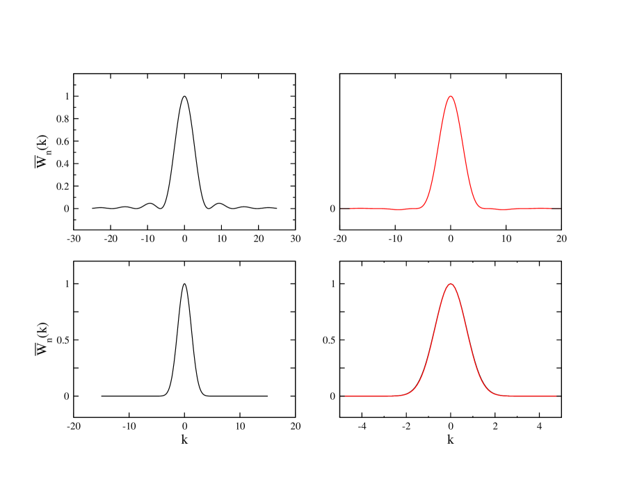
Figure 1: We show the dynamics of the collision process: the tracer particle characteristic function, conditioned that exactly $n$ collision events have occurred, $\bar{W}_{n}(k)$ versus $k$. The velocity PDF of the bath particle is uniform and $\epsilon=0.01$. We show $n=1$ (top left), $n=3$ (top right), $n=10$ (bottom left) and $n=100$ $n=1000$ (bottom right). For the latter case we have $\bar{W}_{100}(k)\simeq\bar{W}_{1000}(k)$, hence the process has roughly converged after $100$ collision events. The equilibrium is well approximated with a Gaussian characteristic function indicating that a Maxwell–Boltzmann equilibrium is obtained.

Remark 1 According to Eq. (10), after a single collision event the PDF of the tracer particle in Fourier space is $\bar{W}_{1}(k)=\bar{f}\left(k\xi_{2}\right)$ provided that $V_{M}(0)=0$. After the second collision event $\bar{W}_{2}(k)=\bar{f}\left(k\xi_{1}\xi_{2}\right)\bar{f}\left(k\xi_{2}\right)$ and after $n$ collision events

$$\bar{W}_{n}(k)=\Pi_{i=1}^{n}\bar{f}\left(k\xi_{1}^{n-i}\xi_{2}\right).$$ (23)

This process is described in Fig. 1, where we show $\bar{W}_{n}(k)$ for $n=1,3,10,100,1000$. In this example we use a uniform distribution of the bath particles PDF Eq. (45), with $\epsilon=0.01$, and $T=1$. After roughly $100$ collision events the characteristic function $\bar{W}_{n}(k)$ reaches a stationary state, which as we will show is well approximated by a Gaussian (i.e., Maxwell–Boltzmann velocity PDF is obtained). Such an equilibrium is not specific to the initial choice of $\bar{f}(k)$, i.e., the assumption of uniform distribution of bath particle velocities. Rather one of my aims is to show that many choices of $\bar{f}(k)$ will flow towards the Gaussian attractor (this resembles flows towards fixed points however now we are working in function space). As we will show these flows do not always belong to the domain of attraction of the Gauss–Maxwell–Boltzmann behavior.

Remark 2 The equilibrium described by Eq. (22) is valid for a larger class of collision models provided that two requirements are satisfied. To see this consider Eq. (12), this equation is clearly not limited to the model under investigation. For example if number of collisions is described by a renewal process, equation (12) is still valid (however generally $P_{n}(t)$ is not described by the Poisson law). The important first requirement is that in the limit $t\to\infty$ $P_{n}(t)$ is peaked around $n\to\infty$, and that $P_{n}(t)$ is not too wide (any renewal process with finite mean satisfies this condition). We may expect that this is the case from standard central limit theorem, and law of large numbers. The second requirement is that recolision of bath particles and tracer particle are not important. This assumption is important since without it the simple form of $\bar{W}_{n}(k)$ is not valid, and hence also Eq. (22). Physically, this means that the bath particles maintain their own equilibrium throughout the collision process, namely fast relaxation to equilibrium of the bath.

Remark 3 The problem of analysis of the equilibrium Eq. (22) is different from the classical mathematical problem of summation of independent identically distributed random variables Feller . The rescaling of $k$ seen in Eq. (22) $k\to k\xi_{1}^{n-i}\xi_{2}$, means that we are treating a problem of summation of independent, though non identical random variables. The number of these random variables is $n$, unlike standard problems of summation of random variables, $n$ also enters in the rescaling of $k$ as seen in $k\xi_{1}^{n-i}\xi_{2}$.

Remark 4 If $m=M$ we find $\bar{W}_{eq}(k)=\bar{f}(k)$, this behavior is expected since in this strong collision limit a single collision event is needed for relaxation of tracer particle to equilibrium. This trivial equilibrium is not stable in the sense that perturbing $\bar{f}(k)$ yields a new equilibrium for the tracer particle.

IV Thermodynamic Approach

In this section the thermodynamic approach is used, imposing the condition that $\bar{W}_{eq}(k)$ is independent of the coupling constant $\epsilon$.

IV.1 Gauss–Maxwell–Boltzmann Equilibrium

We investigate the cumulant expansion of $\bar{W}_{eq}(k)$, assuming that moments of the bath particle velocity PDF are finite. We also assume that $f(\tilde{v}_{m})$ is even as might be expected from symmetry, and from the requirement that the total momentum of the bath is zero.

We use the long wave length expansion

$$\bar{f}(k)=1-{k^{2}\over 2}\langle\tilde{v}_{m}^{2}\rangle+{k^{4}\over 4!}\langle\tilde{v}_{m}^{4}\rangle+O(k^{6}),$$ (24)

where $\langle\tilde{v}_{m}^{2}\rangle$ ($\langle\tilde{v}_{m}^{4}\rangle$) are the second (forth) moment of bath particles velocity. Using Eq. (22)

$$\ln\left[\bar{W}_{eq}\left(k\right)\right]=\lim_{n\to\infty}\sum_{i=1}^{n}\ln\left[\bar{f}\left(k\xi_{1}^{n-i}\xi_{2}\right)\right].$$ (25)

Inserting Eq. (24) in (25) we obtain

$$\ln\left[\bar{W}_{eq}\left(k\right)\right]=-{\langle\tilde{v}_{m}^{2}\rangle\over 2}g_{2}^{\infty}(\epsilon)k^{2}+{\langle\tilde{v}_{m}^{4}\rangle-3\langle\tilde{v}_{m}^{2}\rangle^{2}\over 4!}g_{4}^{\infty}(\epsilon)k^{4}+O(k^{6}).$$ (26)

Using Eq. (20) with $\alpha=2$ we obtain in the limit $\epsilon\to 0$

$$\ln\left[\bar{W}_{eq}\left(k\right)\right]=-{\langle\tilde{v}_{m}^{2}\rangle\over 2}{m\over M}k^{2}+{\langle\tilde{v}_{m}^{4}\rangle-3\langle\tilde{v}_{m}^{2}\rangle^{2}\over 4!}2\left({m\over M}\right)^{3}k^{4}+O\left(k^{6}\right),$$ (27)

where the dependence on mass ratio $m/M$ was explicitly included. To obtain equilibrium using the thermodynamic approach, we require that $\bar{W}_{eq}(k)$ be independent of the mass ratio $\epsilon$. From this physical requirement and Eq. (27) we obtain a standard relationship

$$\langle\tilde{v}_{m}^{2}\rangle={T_{2}\over m}.$$ (28)

This requirement and Eq. (27) means that dependence of mean square velocity of tracer particle and bath particle scale with their masses in a similar way, i.e., like $1/m$ and $1/M$ respectively. In Eq. (28) $T_{2}$ is the temperature, below we show that using similar arguments for power law case leads to a generalized temperature $T_{\alpha}$. We further demand that the forth moment of $f(\tilde{v}_{m})$ will scale with the mass of the bath particle like

$$\langle\tilde{v}_{m}^{4}\rangle=q_{4}\left({T_{2}\over m}\right)^{2},$$ (29)

where $q_{4}$ is a dimensionless constant. This imposed condition results in a velocity PDF for the tracer particle, which is independent of $q_{4}$ and hence of details of bath particle velocity PDF. In this case the equilibrium properties of the tracer particle become independent of the details of $f\left(\tilde{v}_{m}\right)$ (e.g., independent of $q_{4}$), other-wise $\bar{W}_{eq}(k)$ is non universal implying that statistical mechanics does not exist in this case. Inserting Eqs. (28,29) in Eq. (27) we obtain

$$\ln\left[\bar{W}_{eq}\left(k\right)\right]=-{T_{2}k^{2}\over 2M}+\left({T_{2}\over M}\right)^{2}{q_{4}-3\over 4!}2\epsilon k^{4}+O\left(k^{6}\right).$$ (30)

It is important to see that the $k^{4}$ term approaches zero when $\epsilon\to 0$, and hence

$$\lim_{\epsilon\to 0}\ln\left[\bar{W}_{eq}(k)\right]=-{T_{2}k^{2}\over 2M}.$$ (31)

Thus the celebrated Maxwell–Boltzmann velocity PDF is found

$$\lim_{\epsilon\to 0}W_{eq}\left(V_{M}\right)={\sqrt{M}\over\sqrt{2\pi T_{2}}}\exp\left(-{MV_{M}^{2}\over 2T_{2}}\right).$$ (32)

Our model exhibits the relation between the central limit theorem and standard thermal equilibrium in a very direct and simple way. The main conditions for thermal equilibrium are that (i) number of collisions needed to reach equilibrium is very large namely $\epsilon$ is small, (ii) collisions are independent, (iii) scaling conditions on velocity moments of bath particles must be satisfied, and (iv) finite variance of velocity of bath particles PDF. In the next subsection we investigate possible power law generalizations of standard equilibrium.

Figure 2: The equilibrium characteristic function of the tracer particle, $\bar{W}_{eq}(k)$ versus $k$. We consider three types of bath particles velocity PDFs (i) exponential (squares), (ii) uniform (circles), and (iii) Gaussian (diamonds). The velocity distribution of the tracer particle $M$ is well approximated by Maxwell’s distribution plotted as the solid curve $\bar{W}_{eq}(k)=\exp\left(-|k|^{2}\right)$. For the numerical results I used: $M=1$, $T_{2}=2$, $n=2000$, and $\epsilon=0.01$.

remark 1 To fully characterize the equilibrium characteristic function $\bar{W}_{eq}(k)$, the cumulant expansion is investigated to infinite order. Let $\tilde{\kappa}_{m,2j}$ $(\kappa_{M,2j})$ be the $2j$ th cumulant of bath particle (tracer particle) velocity, e.g. $\tilde{\kappa}_{m,2}=\langle\tilde{v}_{m}^{2}\rangle$, $\tilde{\kappa}_{m,4}=\langle\tilde{v}_{m}^{4}\rangle-\langle\tilde{v}_{m}^{2}\rangle^{2}$, etc. Then using Eq. (22) one can show that

$$\kappa_{M,2j}=g_{2j}^{\infty}\left(\epsilon\right)\tilde{\kappa}_{m,2j}.$$ (33)

Since $g_{2j}^{\infty}(1)=1$ we find $\kappa_{M,2j}=\tilde{\kappa}_{m,2j}$ if $m=M$, and hence for that case $\bar{W}_{eq}(k)=\bar{f}(k)$ as mentioned previously. We assume that scaling properties of bath particles follow $\tilde{\kappa}_{m,2j}=c_{2j}T_{2}^{j}/m^{j}$, where $c_{2j}$ are dimensionless parameters which depend on $f(\tilde{v}_{m})$, $j=1,2,\cdots$, and $c_{2}=1$. The parameters $c_{2j}$ for $j>1$ are the irrelevant parameters of the model in the limit of weak collisions. To see this note that when $\epsilon\to 0$ we have $\kappa_{M,2j}=(T_{2}/M)\delta_{j1}$ implying relaxation to a unique thermal equilibrium which is independent of the choice of bath particle velocity distribution.

Remark 2 Instead of the condition Eq. (29) it is sufficient to demand that the forth moment of bath particle velocity will scale with the mass of the bath particles like $\langle\tilde{v}_{m}^{4}\rangle\propto{1\over m^{\theta}}$ and $0<\theta<3$. If $\langle\tilde{v}_{m}^{4}\rangle\propto{1\over m^{3}}$ for example, we find that the second term in Eq. (27) does not vanish in the limit $\epsilon\to 0$. In this case the equilibrium of the tracer particle will be sensitive to behavior of $f(\tilde{v}_{m})$, and hence will exhibit a non-universal behavior.

Figure 3: The tracer particle’s equilibrium characteristic function, for the case when the velocity of the bath particles is exponentially distributed Eq. (43). The parameters are the same as in Fig. 2 however now $\epsilon$ is varied. I use $\epsilon=0.05$ (diamonds), $\epsilon=0.01$ (squares), $\epsilon=0.001$ (circles). As $\epsilon$ approaches zero, number of collisions needed to reach an equilibrium becomes very large and then Maxwell–Boltzmann thermal equilibrium is obtained, the solid curve $\bar{W}_{eq}(k)=\exp(-k^{2})$. Note the logarithmic scale of the figure.

IV.2 Lévy type of Equilibrium

We now assume that the bath particle velocity PDF is even with zero mean, and that it decays like a power law $P(\tilde{v}_{m})\propto|\tilde{v}_{m}|^{-(1+\alpha)}$ when $\tilde{v}_{m}\to\infty$ where $0<\alpha<2$. In this case the variance of velocity distribution diverges. We use the small $k$ expansion of the bath particle characteristic function

$$\bar{f}\left(k\right)=1-{A_{\alpha}|k|^{\alpha}\over\Gamma\left(1+\alpha\right)}+{B|k|^{\beta}\over\Gamma\left(1+\beta\right)}+o\left(|k|^{\beta}\right)$$ (34)

with $\alpha<\beta\leq 2\alpha$. Using Eq. (25) we find

$$\ln\left[\bar{W}_{eq}\left(k\right)\right]=\left\{\begin{array}[]{l l}-{A_{\alpha}\over\Gamma\left(1+\alpha\right)}g_{\alpha}^{\infty}\left(\epsilon\right)|k|^{\alpha}+{B\over\Gamma\left(1+\beta\right)}g_{\beta}^{\infty}\left(\epsilon\right)|k|^{\beta}&\beta<2\alpha\\ &\ \mbox{}\\ -{A_{\alpha}\over\Gamma\left(1+\alpha\right)}g_{\alpha}^{\infty}\left(\epsilon\right)|k|^{\alpha}+\left[{B\over\Gamma\left(1+2\alpha\right)}-{A^{2}\over 2\Gamma^{2}\left(1+\alpha\right)}\right]g_{2\alpha}^{\infty}\left(\epsilon\right)|k|^{2\alpha}&\beta=2\alpha\\ \end{array}\right.$$ (35)

where terms of order higher than $|k|^{\beta}$ are neglected. Using Eq. (17) we obtain in the limit $\epsilon\to 0$

$$\ln\left[\bar{W}_{eq}\left(k\right)\right]\sim\left\{\begin{array}[]{l l}-{A_{\alpha}\over\Gamma\left(1+\alpha\right)}\left({m\over M}\right)^{\alpha-1}{2^{\alpha-1}\over\alpha}|k|^{\alpha}+{B\over\Gamma\left(1+\beta\right)}\left({m\over M}\right)^{\beta-1}{2^{\beta-1}\over\beta}|k|^{\beta}&\beta<2\alpha\\ &\\ -{A_{\alpha}\over\Gamma\left(1+\alpha\right)}\left({m\over M}\right)^{\alpha-1}{2^{\alpha-1}\over\alpha}|k|^{\alpha}+\left[{B\over\Gamma\left(1+2\alpha\right)}-{A^{2}\over 2\Gamma^{2}\left(1+\alpha\right)}\right]\left({m\over M}\right)^{2\alpha-1}{2^{2\alpha-1}\over 2\alpha}|k|^{2\alpha}&\beta=2\alpha.\end{array}\right.$$ (36)

To obtain an equilibrium we use the thermodynamical argument. We require that equilibrium velocity PDF of the tracer particle $M$ be independent of the mass of the bath particle, as we did for the Maxwell–Boltzmann case Eq. (28). This condition yields

$$A_{\alpha}={T_{\alpha}\over m^{\alpha-1}},$$ (37)

where within the context of our model $T_{\alpha}$ has a meaning of generalized temperature whose units are $\mbox{Kg}^{\alpha-1}\mbox{Mt}^{\alpha}/\mbox{Sec}^{\alpha}$. An additional requirement is needed to obtain a unique equilibrium (i.e., an equilibrium which does not depend on details of bath particle velocity PDF like $B$): terms beyond the $|k|^{\alpha}$ term in Eq. (36) must vanish in the limit $\epsilon\to 0$. This occurs for a large family of velocity PDFs $f\left(\tilde{v}_{m}\right)$ which satisfy the condition

$$B\propto{1\over m^{\theta}}$$ (38)

and now $\theta<\beta-1$. For the Gauss-Maxwell-Boltzmann case considered in previous section we had $\beta=4$ while now $\beta<4$. Using this condition we obtain

$$\lim_{\epsilon\to 0}\ \ln\left[\bar{W}_{eq}\left(k\right)\right]=-{T_{\alpha}2^{\alpha-1}\over\Gamma\left(1+\alpha\right)\alpha M^{\alpha-1}}|k|^{\alpha},$$ (39)

hence Lévy type of equilibrium is obtained

$$\lim_{\epsilon\to 0}W_{eq}\left(V_{M}\right)=\left[{\Gamma\left(1+\alpha\right)M^{*(\alpha-1)}\over T_{\alpha}}\right]^{1/\alpha}l_{\alpha}\left\{\left[{\Gamma\left(1+\alpha\right)M^{*(\alpha-1)}\over T_{\alpha}}\right]^{1/\alpha}V_{M}\right\}$$ (40)

where $M^{*}=M\alpha^{1/(\alpha-1)}/2$ is the renormalized mass. For $\alpha=2$ the Maxwell–Boltzmann PDF Eq. (32) is recovered and $M^{*}=M$.

From physical requirements we note that our results are valid only when $1<\alpha\leq 2$. If $\alpha=1$ the velocity PDF becomes independent of the mass of the tracer particle, while when $\alpha<1$ the heavier the tracer particle the faster its motion (in statistical sense). This implies that imposing the condition of independence of tracer particle velocity PDF on the coupling constant, based on the thermodynamic argument, is not the correct path. This is one of the reasons why I consider a scaling approach in the next section. The unphysical behavior also indicates that the assumption of uniform collision rate is unphysical when $\langle|\tilde{v}_{m}|\rangle=\infty$, implying that the mean field approach we are using breaks down when $\alpha\leq 1$.

Remark 1 The domain of attraction of the Lévy equilibrium we find, Eq. (40) does not include all power law distribution with $\alpha<2$. Consider for example

$$\bar{f}(k)={1\over 2}\left\{\exp\left[-{2T_{\alpha}|k|^{\alpha}\over m^{\alpha-1}\Gamma\left(1+\alpha\right)}\right]+\exp\left(-{T_{2}k^{2}\over m}\right)\right\},$$ (41)

hence the gas particle velocity distribution in this case is a sum of a Gaussian and a Lévy distributions. The small $k$ expansion of Eq. (41) is

$$\bar{f}(k)=1-{T_{\alpha}|k|^{\alpha}\over m^{\alpha-1}\Gamma\left(1+\alpha\right)}-{T_{2}k^{2}\over 2m}\cdots,$$ (42)

where we consider $1<\alpha<2$. Using Eqs. (34,42) we find $\beta=2$, while comparing Eq. (38) and Eq. (42) yields $\theta=1$. Now the condition $\theta<\beta-1$ does not hold, and hence the Lévy equilibrium Eq. (40) is not obtained. Interestingly, one can show that for this case one obtains an equilibrium characteristic function $\bar{W}_{eq}(k)$ which is a convolution of a Lévy PDF and a Gaussian PDF. I suspect that this type of equilibrium is not limited to this example.

IV.3 Numerical Examples

To demonstrate the results exact solutions of the problem are investigated. This yields insight into convergence rate to stable equilibrium.

IV.3.1 Maxwell Statistics

First consider the Maxwell–Boltzmann case. We investigate three types of bath particle velocity PDFs:
$(i)$ The exponential

$$f\left(\tilde{v}_{m}\right)={\sqrt{2m}\over 2\sqrt{T_{2}}}\exp\left(-{\sqrt{2m}|\tilde{v}_{|}\over\sqrt{T_{2}}}\right),$$ (43)

which yields

$$\bar{f}(k)={1\over 1+{T_{2}k^{2}\over 2m}}.$$ (44)

$(ii)$ The uniform PDF

$$f(\tilde{v}_{m})=\left\{\begin{array}[]{l l}\sqrt{{m\over 12T_{2}}}&\mbox{if}\ |\tilde{v}_{m}|<\sqrt{{3T_{2}\over m}}\\ &\\ 0&\ \mbox{otherwise}\\ \end{array}\right.$$ (45)

which yields

$$\bar{f}(k)={\sin\left(\sqrt{{3T_{2}\over m}}k\right)\over\sqrt{{3T_{2}\over m}}k}.$$ (46)

$(iii)$ The Gaussian PDF

$$\bar{f}(k)=\exp\left(-{k^{2}T_{2}\over 2m}\right).$$ (47)

The small $k$ expansion of Eqs. (44,46,47) is $\bar{f}(k)\sim 1-k^{2}T_{2}/(2m)+\cdots$, indicating that the second moment of velocity of bath particles $\langle\tilde{v}_{m}^{2}\rangle$ is identical for the three PDFs.

To obtain numerically exact solution of the problem we use Eq. (22) with large though finite $n$. In all our numerical examples we used $M=1$ hence $m=\epsilon$. Thus for example for the uniform velocity PDF Eq. (46) we have

$$\bar{W}_{eq}\left(k\right)\simeq\exp\left\{\sum_{i=1}^{n}\ln\left[\sqrt{{\epsilon\over 3T_{2}}}{\sin\left(k\sqrt{{3T_{2}\over m}}\left({1-\epsilon\over 1+\epsilon}\right)^{n-i}{2\epsilon\over 1+\epsilon}\right)\over k\left({1-\epsilon\over 1+\epsilon}\right)^{n-i}{2\epsilon\over 1+\epsilon}}\right]\right\}.$$ (48)

To obtain equilibrium we increase $n$ for a fixed $\epsilon$ and temperature until a stationary solution is obtained.

According to our analytical results the bath particle velocity PDFs Eqs. (43,45,47), belong to the domain of attraction of the Maxwell–Boltzmann equilibrium. In Fig. 2 we show $\bar{W}_{eq}(k)$ obtained from numerical solution of the problem. The numerical solution exhibits an excellent agreement with the Maxwell–Boltzmann equilibrium. Thus details of the precise shape of velocity PDF of bath particles are unimportant, and as expected the Maxwell-Boltzmann distribution is stable. To obtain the results in Fig. 2 I used $\epsilon=0.01$, $T_{2}=2$, $M=1$ and $n=2000$. For convenience Fourier space is used, the solid curve is theoretical prediction $\ln[W_{eq}(k)]=-k^{2}$ which is strictly valid in the limit $n\to\infty$ and then $\epsilon\to 0$.

A closer look at $\bar{W}_{eq}(k)$ reveals that for large $k$ deviations from Gaussian behavior are found for finite values of $\epsilon$, as might be expected. In Fig. 3 we show the numerically exact solution using the exponential velocity PDF Eq. (43) and vary the mass ratio $\epsilon$. The figure demonstrates that when $\epsilon\to 0$ the asymptotic theory becomes exact, the convergence rate depends on the value of $k$. As we noted already the Maxwell–Boltzmann statistics is reached only if number of collisions needed to obtain an equilibrium is very large, which implies small values of $\epsilon$.

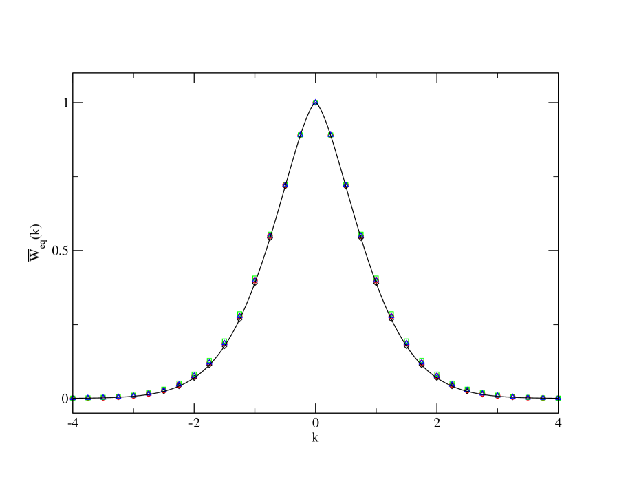
Figure 4: The equilibrium characteristic function $\bar{W}_{eq}(k)$, for the case when velocities of bath particles are distributed according to a power law with $\alpha=3/2$. Four types of bath particles characteristic functions are considered: (i) the Hyper-geometric function Eq. (49) (squares), (ii) Meijer G function Eq. (51), (circles), (iii) Bessel function Eq. (53), (triangles), and (iv) the Holtsmark function Eq. (55) (diamonds). For all these cases, the equilibrium characteristic function $\bar{W}_{eq}(k)$ is well approximated by the Lévy characteristic function; the solid curve $\bar{W}_{eq}(k)=\exp\left(-2^{3/2}|k|^{3/2}/3\right)$. For the numerical results we used: $M=1$, $T_{\alpha}=\Gamma(5/2)$, $\epsilon=5e-5$, and $n=1e6$.

IV.3.2 Lévy Statistics

We now consider four power law PDFs satisfying $f\left(\tilde{v}_{m}\right)\propto|\tilde{v}_{m}|^{-5/2}$, namely $\alpha=3/2$.
$(i)$ Case $1$ we choose

$$f\left(\tilde{v}_{m}\right)={N_{1}\over\left(1+c_{1}|\tilde{v}_{m}|\right)^{5/2}},$$ (49)

with $c_{1}=\left(3\pi\right)^{2/3}m^{1/3}2^{-1}(T_{3/2})^{2/3}$ and $N_{1}=3c_{1}/4$. The characteristic function is given in terms of a Hyper-geometric function Math

$$\bar{f}(k)=\frac{4N_{1}\,\left(c_{1}^{\frac{3}{2}}\,\mbox{HypergeometricPFQ}(\{1\},\{-\left(\frac{1}{4}\right),\frac{1}{4}\},\frac{-k^{2}}{4\,c_{1}^{2}})-{|k|}^{\frac{3}{2}}\,{\sqrt{2\,\pi}}\,\left(\cos(\frac{k}{c_{1}})+\mbox{Sign}(k)\,\sin(\frac{k}{c_{1}})\right)\right)}{3\,c_{1}^{\frac{5}{2}}}.$$ (50)

$(ii)$ Case $2$

$$f\left(\tilde{v}_{m}\right)={N_{2}\over 1+c_{2}|\tilde{v}_{m}|^{5/2}},$$ (51)

where $c_{2}=(2\sqrt{2\pi m})^{5/3}(3GT_{3/2})^{-5/3}$, $G=(4\pi/5)\sqrt{2/(5+\sqrt{5})}$, $N_{2}=c_{2}^{2/5}/(2G)$. The characteristic function is expressed in terms of Meijer G function Math

$$\bar{f}(k)=\frac{2N_{2}\mbox{MeijerG}(\{\{\frac{3}{20},\frac{2}{5},\frac{13}{20}\},\{\}\},\{\{0,\frac{3}{20},\frac{1}{5},\frac{2}{5},\frac{2}{5},\frac{3}{5},\frac{13}{20},\frac{4}{5},\frac{9}{10}\},\{\frac{1}{10},\frac{3}{10},\frac{1}{2},\frac{7}{10}\}\},\frac{k^{10}}{10000000000\,c_{2}^{4}})}{4\,{\sqrt{5}}\,c_{2}^{\frac{2}{5}}\,{\pi}^{\frac{5}{2}}}.$$ (52)

To obtain $\bar{W}_{eq}(k)$ we used the numerical Fourier transform of Eqs. (49,51), instead of the rather formal exact expressions Eqs. (50,52).
(iii) Case $3$

$$f\left(\tilde{v}_{m}\right)={N_{3}\over\left(1+C_{3}\tilde{v}_{m}^{2}\right)^{5/4}}$$ (53)

where $C_{3}=\{\Gamma[1/4]\Gamma[5/2]\sqrt{2m}3^{-1}T_{3/2}^{-1}\Gamma^{-1}(3/4)]\}^{4/3}$, $N_{3}=0.75T_{3/2}\Gamma^{-1}(5/2)(2\pi m)^{-1/2}C_{3}^{5/4}$. The characteristic function is

$$\bar{f}(k)=N_{3}C_{3}^{-7/8}{2^{1/4}\sqrt{\pi}\over\Gamma\left({5\over 4}\right)}|k|^{3/4}K_{3/4}\left({|k|\over\sqrt{C_{3}}}\right),$$ (54)

where $K_{3/4}$ is the modified Bessel function of the second kind.
$(iv)$ Case $4$ the Lévy PDF with index $3/2$ whose Fourier pair is

$$\bar{f}\left(k\right)=\exp\left[-{T_{3/2}|k|^{5/2}\over\sqrt{m}\Gamma\left(5/2\right)}\right].$$ (55)

The $|\tilde{v}_{m}|\to\infty$ behavior of the PDFs (49-55) is

$$f\left(\tilde{v}_{m}\right)\sim{3T_{3/2}\over 4\sqrt{2\pi m}}|\tilde{v}_{m}|^{-5/2},$$ (56)

hence the small $k$ behavior of the characteristic function is

$$\bar{f}\left(k\right)\sim 1-{T_{3/2}|k|^{3/2}\over\sqrt{m}\Gamma\left(5/2\right)}.$$ (57)

According to our results in previous section the velocity PDFs Eqs. (49-51) belong to the domain of attraction of the Lévy type of equilibrium

$$\lim_{\epsilon\to 0}\bar{W}_{eq}\left(k\right)=\exp\left[-{T_{3/2}2^{3/2}\over\sqrt{M}3\Gamma\left(5/2\right)}|k|^{3/2}\right].$$ (58)

Namely, $W_{eq}\left(V_{M}\right)$ is the Lévy PDF with index $3/2$ also called the Holtsmark PDF.

Figure 5: The tracer particle equilibrium characteristic function, for the case when the characteristic function of the bath particles is described by the Bessel function Eq. (54). The parameters are the same as in Fig. 4 however now $\epsilon$ is varied. We use $\epsilon=10^{-3}$ (diamonds), $\epsilon=10^{-4}$ (squares), $\epsilon=10^{-5}$ (circles), and $\epsilon=10^{-6}$ (stars). As $\epsilon$ approaches zero, number of collisions needed to reach an equilibrium becomes very large and then a Lévy type of equilibrium is obtained, the solid curve $\bar{W}_{eq}(k)=\exp\left(-2^{3/2}|k|^{3/2}/3\right)$. Note the logarithmic scale of the figure.

Similar to the Maxwell-Boltzmann case, numerically exact solution are obtained, in $k$ space using Eq. (22) with finite $n$. For example for the power law velocity PDF Eq. (53) we use

$$\bar{W}_{eq}\left(k\right)\simeq$$

$$\exp\left\{\sum_{i=1}^{n}\log\left[N_{3}C_{3}^{-7/8}{2^{1/4}\sqrt{\pi}\over\Gamma\left(5/4\right)}|k|^{3/4}\left({1-\epsilon\over 1+\epsilon}\right)^{3(n-i)/4}\left({2\epsilon\over 1+\epsilon}\right)^{3/4}K_{3/4}\left(\left({1-\epsilon\over 1+\epsilon}\right)^{n-i}|k|{2\epsilon\over 1+\epsilon}\left(C_{3}\right)^{-1/2}\right)\right]\right\},$$ (59)

where we fix $\epsilon$ and $T_{3/2}$ and increase $n$ until a stationary solution is obtained.

In Fig. 4 we show $\bar{W}_{eq}(k)$ obtained using numerically exact solution based on the four PDFs Eqs. (49,51,53,55). The exact solutions are in good agreement with the theoretical prediction Eq. (58). Thus, similar to the Maxwell–Boltzmann case, the exact shape of the equilibrium distribution does not depend on the details of the velocity PDF of the bath particles (besides $\alpha$ and $T_{\alpha}$ of-course).

A closer look at $\bar{W}_{eq}(k)$ reveals that for large $k$ deviations from Lévy behavior are found for finite values of $\epsilon$, similar to what we have shown for the Gaussian case Fig. 3. In Fig. 5 we show the numerically exact solution using the power law velocity PDF Eq. (53) and vary the mass ratio $\epsilon$. The figure demonstrates that when $\epsilon\to 0$ the asymptotic theory becomes exact, the convergence rate depends on the value of $k$. The Lévy type of equilibrium is reached only if number of collisions needed to obtain an equilibrium is very large, which implies small values of $\epsilon$. The convergence towards a stable equilibrium was found to be slow compared with the Gaussian case (for $\epsilon=1e-6$ we used $n=3e6$ to obtain a stationary solution).

We also consider the marginal case $\alpha=1$, which marks the transition from finite $\langle|\tilde{v}_{m}|\rangle$ for $\alpha>1$ to infinite value of $\langle|\tilde{v}_{m}|\rangle$ for $\alpha<1$. We considered the velocity PDF

$$f\left(\tilde{v}_{m}\right)={1\over 2\left(1+|\tilde{v}_{m}|\right)^{2}}.$$ (60)

The characteristic function is Math

$$\bar{f}\left(k\right)=\frac{\mbox{MeijerG}(\{\{0\},\{\}\},\{\{0,\frac{1}{2},1\},\{\}\},\frac{k^{2}}{4})}{{\sqrt{\pi}}},$$ (61)

which for small $k$ behaves like $\bar{f}\left(k\right)=1-\pi|k|/2\cdots$. According to the theory in the limit $\epsilon\to 0$

$$\bar{W}_{eq}(k)=\exp(-\pi|k|/2).$$ (62)

Thus the velocity PDF of the tracer particle $M$ is the Lorentzian density. As mentioned in this case the equilibrium obtained is independent of mass $M$. In Fig. 6 we show the numerically exact solution of $\bar{W}_{eq}\left(k\right)$ for several mass ratios $\epsilon$. As $\epsilon\to 0$ we obtain the predicted Lévy type of equilibrium.

Figure 6: The equilibrium characteristic function, for a case when the velocity of the bath particles is a power law with $\alpha=1$ Eq. (60). We use $\epsilon=0.01$ (squares), $\epsilon=0.001$ (diamonds), $\epsilon=0.0005$ (circles). As $\epsilon$ approaches zero, number of collisions needed to reach an equilibrium becomes very large and then a Lévy type of thermal equilibrium is obtained: the solid curve $\bar{W}_{eq}(k)=\exp(-\pi|k|/2)$. Note the logarithmic scale of the figure.

V Scaling Approach: the Relevant Scale is Energy

A second approach to the problem is now considered. We assume that statistical properties of bath particles velocities can be characterized with an energy scale $T$. Since $T$, $m$ and $\tilde{v}_{m}$ are the only variables describing the bath particle we have

$$f\left(\tilde{v}_{m}\right)={1\over\sqrt{T/m}}q\left({\tilde{v}_{m}\over\sqrt{T/m}}\right).$$ (63)

We also assume that $f(\tilde{v}_{m})$ is an even function, as expected from symmetry. The dimensionless function $q(x)\geq 0$ satisfies a normalization condition

$$\int_{-\infty}^{\infty}q(x){\rm d}x=1,$$ (64)

otherwise it is rather general. The scaling assumption made in Eq. (63) is very natural, since the total energy of bath particles is nearly conserved, i.e. the energy transfer to the single heavy particle being much smaller than the total energy of the bath particles. From this starting point we investigate now equilibrium properties of the tracer particle $M$. Showing among other things that $T$ has the meaning of temperature.

V.1 Gauss–Maxwell–Boltzmann Distribution

We first consider the case where moments of $f\left(\tilde{v}_{m}\right)$ are finite. The second moment of the bath particle velocity is

$$\langle\tilde{v}_{m}^{2}\rangle={T\over m}\int_{-\infty}^{\infty}x^{2}q(x){\rm d}x.$$ (65)

Without loss of generality we set $\int_{-\infty}^{\infty}x^{2}q(x){\rm d}x=1$. The scaling behavior Eq. (63) and the assumption of finiteness of moments of the PDF yields

$$\langle\tilde{v}_{m}^{2n}\rangle=\left({T\over m}\right)^{n}q_{2n},$$ (66)

where the moments of $q(x)$ are defined according to

$$q_{2n}=\int_{-\infty}^{\infty}x^{2n}q(x){\rm d}x.$$ (67)

Thus the small $k$ expansion of the characteristic function is

$$\bar{f}\left(k\right)=1-{Tk^{2}\over 2m}+q_{4}\left({T\over m}\right)^{2}{k^{4}\over 4!}+O(k^{6}).$$ (68)

Inserting Eq. (68) in Eq. (22) we obtain

$$\ln\left[\bar{W}_{eq}\left(k\right)\right]=-{T\over 2m}g_{2}^{\infty}\left(\epsilon\right)k^{2}+{q_{4}-3\over 4!}\left({T\over m}\right)^{2}g_{4}^{\infty}\left(\epsilon\right)k^{4}+O(k^{6}).$$ (69)

In the limit $\epsilon\to 0$ the second term on the right hand side of Eq. (69) is zero, using Eq. (18)

$$\lim_{\epsilon\to 0}\ln\left[\bar{W}_{eq}\left(k\right)\right]=-{T\over 2M}k^{2}.$$ (70)

The parameters $q_{2n}$ with $n>1$ are the irrelevant parameters of the problem. From Eq. (70) it is easy to see that the Maxwell–Boltzmann velocity PDF for the tracer particle $M$ is obtained.

V.2 Lévy Velocity Distribution

Now we assume that the variance of $f\left(\tilde{v}_{m}\right)$ diverges, i.e., $q(x)\propto|x|^{-(1+\alpha)}$ when $|x|\to\infty$ and $0<\alpha<2$. For this case the bath particle characteristic function is

$$\bar{f}\left(k\right)=1-{q_{\alpha}\over\Gamma\left(1+\alpha\right)}\left({T\over m}\right)^{\alpha/2}|k|^{\alpha}+{q_{\beta}\over\Gamma\left(1+\beta\right)}\left({T\over m}\right)^{\beta/2}|k|^{\beta}+o(|k|^{\beta})$$ (71)

where $\alpha<\beta\leq 2\alpha$. In many cases $\beta=2$, an example is given in next subsection. $q_{\alpha}$ and $q_{\beta}$ are dimensionless numbers which depend of-course on $q(x)$. Without loss of generality we may set $q_{\alpha}=1$. In Eq. (71) we have used the assumption that $f(\tilde{v}_{m})$ is even.

Using the same technique used in previous section we obtain the equilibrium characteristic function for the tracer particle $M$

$$\ln\left[\bar{W}_{eq}\left(k\right)\right]=\left\{\begin{array}[]{l l}-{1\over\Gamma\left(1+\alpha\right)}\left({T\over m}\right)^{\alpha/2}g_{\alpha}^{\infty}\left(\epsilon\right)|k|^{\alpha}+{q_{\beta}\over\Gamma\left(1+\beta\right)}\left({T\over m}\right)^{\beta/2}g_{\beta}^{\infty}\left(\epsilon\right)|k|^{\beta}&\beta<2\alpha\\ &\ \mbox{}\\ -{1\over\Gamma\left(1+\alpha\right)}\left({T\over m}\right)^{\alpha/2}g_{\alpha}^{\infty}\left(\epsilon\right)|k|^{\alpha}+\left[{q_{2\alpha}\over\Gamma\left(1+2\alpha\right)}-{1\over 2\Gamma^{2}\left(1+\alpha\right)}\right]\left({T\over m}\right)^{\alpha}g_{2\alpha}^{\infty}\left(\epsilon\right)|k|^{2\alpha}&\beta=2\alpha.\\ \end{array}\right.$$ (72)

Taking the small $\epsilon$ limit the following expansions are found, if $\beta<2\alpha$

$$\ln\left[\bar{W}_{eq}\right(k\left)\right]\sim-{2^{\alpha-1}\over\alpha\Gamma\left(1+\alpha\right)}\left({T\over M}\right)^{\alpha/2}{|k|^{\alpha}\over\epsilon^{1-\alpha/2}}+{q_{\beta}2^{\beta-1}\over 2\Gamma\left(1+\beta\right)}\left({T\over M}\right)^{\beta/2}{|k|^{\beta}\over\epsilon^{1-\beta/2}}+o(|k|)^{\beta},$$ (73)

if $\beta=2\alpha$

$$\ln\left[\bar{W}_{eq}\right(k\left)\right]\sim-{2^{\alpha-1}\over\alpha\Gamma\left(1+\alpha\right)}\left({T\over M}\right)^{\alpha/2}{|k|^{\alpha}\over\epsilon^{1-\alpha/2}}+\left[{q_{\beta}\over\Gamma\left(1+\beta\right)}-{1\over 2\Gamma^{2}\left(1+\alpha\right)}\right]\left({T\over M}\right)^{\alpha}{2^{2\alpha-1}\over 2\alpha}{|k|^{2\alpha}\over\epsilon^{1-\alpha}}+o(|k|^{2\alpha}).$$ (74)

Thus for example if $\beta=2$ the leading term in Eq. (73) scales with $\epsilon$ according to $\epsilon^{\alpha/2-1}\to\infty$, while the second term scales like $\epsilon^{0}$. Thus from Eqs. (73,74) we see when $\epsilon$ is small and $k$ not too large, we may neglect the second and higher order terms. This yields a Lévy type of behavior

$$\bar{W}_{eq}\left(k\right)\sim\exp\left[-{2^{\alpha-1}\over\alpha\Gamma\left(1+\alpha\right)}\left({T\over M}\right)^{\alpha/2}{|k|^{\alpha}\over\epsilon^{1-\alpha/2}}\right].$$ (75)

We note that for $\alpha\neq 2$ the equilibrium Eq. (75) depends on $\epsilon$. While for the Maxwell–Boltzmann case $\alpha=2$, the equilibrium is independent of the coupling constant $\epsilon$. This difference between the Lévy equilibrium and the Maxwell–Boltzmann equilibrium is related to the conservation of energy and momentum during a collision event, and to the fact that the energy of the particles is quadratic in their velocities. The asymptotic behavior Eq. (75) is now demonstrated using numerical examples.

Figure 7: We show the equilibrium characteristic function of the tracer particle, using the scaling approach. Numerically exact solution of the problem are obtained using three long tailed bath particle velocity PDFs (i) Eq. (76) squares, (ii) Eq. (77) triangles, (iii) Eq. (82) diamonds. The tracer particle equilibrium is well approximated by the Lévy characteristic function the solid curve; $\bar{W}_{eq}(k)\sim\exp\left(-2.211|{k\over\epsilon^{1/6}}|^{3/2}\right)$. For the numerical results we used $T=4.555$, $\epsilon=1e-5$ and $M=1$.

V.3 Numerical Examples:- Lévy Equilibrium

We consider three types of bath particle velocity PDFs, for large values of $|v_{m}|\to\infty$ these PDFs exhibit $f\left(\tilde{v}_{m}\right)\propto|\tilde{v}_{m}|^{-5/2}$, which implies $\alpha=3/2$.
(i) Case 1

$$f\left(\tilde{v}_{m}\right)={N_{1}\over\left(1+c\sqrt{{m\over T}}|\tilde{v}_{m}|\right)^{5/2}},$$ (76)

where the normalization constant is $N_{1}=c3\sqrt{m/T}/4$ and $c=3^{2/3}/2$. The Fourier transform of this equation can be expressed in terms of a Hyper-geometric function as in Eq. (50).
(ii) Case 2,

$$f\left(\tilde{v}_{m}\right)={N_{2}\over\left(1+{m\tilde{v}_{m}^{2}\over 2\tilde{T}}\right)^{5/4}}$$ (77)

for $-\infty<\tilde{v}_{m}<\infty$. The normalization constant is

$$N_{2}=\sqrt{{m\over 2\tilde{T}}}{\Gamma\left({1\over 4}\right)\over 4\sqrt{\pi}\Gamma\left({3\over 4}\right)},$$ (78)

and

$$\tilde{T}={2\over\pi^{2/3}}\left[{\Gamma\left({3\over 4}\right)\over\Gamma\left({1\over 4}\right)}\right]^{4/3}T.$$ (79)

The bath particle characteristic function is

$$\bar{f}\left(k\right)={2^{1/4}N\sqrt{\pi}\over\Gamma\left(5/4\right)\left({m\over 2\tilde{T}}\right)^{7/8}}|k|^{3/4}K_{3/4}\left({k\sqrt{2\tilde{T}}\over\sqrt{m}}\right),$$ (80)

which yields the small $k$ expansion

$$\bar{f}\left(k\right)=1-2.34565\left({\tilde{T}\over m}\right)^{3/4}|k|^{3/2}+2{\tilde{T}\over m}k^{2}+\cdots,$$ (81)

or using Eq. (79) $\bar{f}\left(k\right)=1-\left(T/m\right)^{3/4}|k|^{3/2}/\Gamma(5/2)+\cdots$.
(iii) Case 3, the bath particle velocity PDF is a Lévy PDF with index $3/2$, whose characteristic function is

$$\bar{f}\left(k\right)=\exp\left[-\left({T\over m}\right)^{3/4}{|k|^{3/2}\over\Gamma\left(5/2\right)}\right].$$ (82)

According to our theory these power law velocity PDFs, yield a Lévy equilibrium for the tracer particle, Eq. (75). In Fig. 7 we show numerically exact solution of the problem for cases (1-3). These solutions show a good agreement between numerical results and the asymptotic theory. The Lévy equilibrium for the tracer particle is not sensitive to precise shape of the velocity distribution of the bath particle, and hence like the Maxwell–Boltzmann equilibrium is stable.

A closer look at $\bar{W}_{eq}(k)$, for finite value of $\epsilon$, reveals expected deviations from Lévy behavior when $k$ is large. In Fig. 8 we obtained the numerical solution of the problem using Eqs. (22) and (80). As in previous sections, we fixed $\epsilon$ and used values of $n$ which were large enough to obtain a stationary solution (e.g., when $\epsilon=1e-6$ we used $n=3e6$). In Fig. 8 we show that as $\epsilon\to 0$ the asymptotic Lévy solution yields an excellent approximation, for a range of $k$ in which the characteristic function $\bar{W}_{eq}(k)$ decays over several order of magnitude.

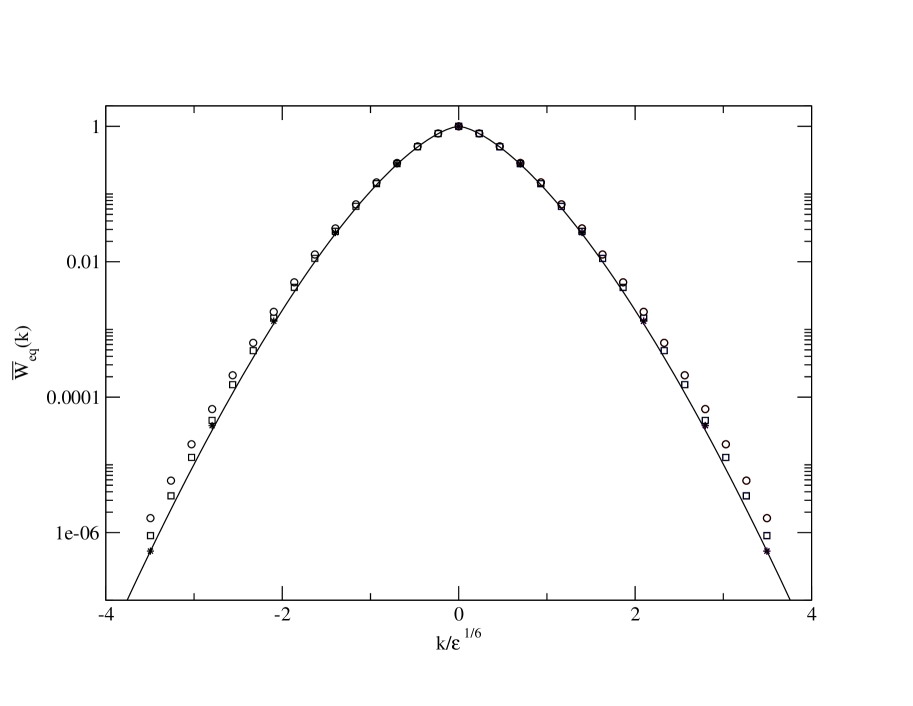
Figure 8: The tracer particle equilibrium characteristic function $\bar{W}_{eq}(k)$ versus $k$. The velocity distribution of the bath particle is described by Eq. (80). The solid curve is the theoretical prediction the Lévy characteristic function $\bar{W}_{eq}(k)\sim\exp\left(-2.211|{k\over\epsilon^{1/6}}|^{3/2}\right)$. We used $\epsilon=1e-4$ (circles), $\epsilon=1e-5$ (squares), and $\epsilon=1e-6$ (stars). As $\epsilon\to 0$ number of collisions needed to reach an equilibrium becomes large and then a Lévy behavior is obtained.

VI Back to Dynamics: Fractional Fokker–Planck Equations

Much work was devoted to the investigation of Langevin equation with Lévy white noise West ; Jep ; Fog ; Vlad ; Garb , or related fractional Fokker–Planck equation Chechkin ; MBK . For example the simplest case of generalized Brownian motion, West and Seshadri West consider

$$\dot{V_{M}}=-\gamma V_{M}+\eta(t)$$ (83)

where $\eta(t)$ is a white Lévy noise. Not surprisingly the equilibrium in this case is a Lévy distribution. While such a stochastic approach might be used to gain some insight also on equilibrium, the approach is clearly limited. If we do not have first principle equilibrium, one cannot impose on the stochastic dynamics the desired stationary solution (i.e., relevant Einstein relation is not known). Hence in several investigations the dissipation $\gamma$ in Eq. (83) is treated as independent of the noise intensity $\eta(t)$. In the context of collision models, this is unphysical, since the collisions are responsible both for the dissipation and the fluctuations. These problems are treated now. Note that fractional Fokker–Planck equations compatible with Boltzmann equilibrium are considered in BS ; BPrl ; Soko .

We consider the fractional Fokker–Planck equation describing the dynamics of the collision model under investigation. We rewrite the kinetic equation (7)

$${\partial\bar{W}(k,t)\over\partial t}=-R\bar{W}(k,t)\left[1-\bar{f}\left(k\xi_{2}\right)\right]+R\left[\bar{W}\left(k\xi_{1},t\right)-\bar{W}\left(k,t\right)\right]\bar{f}\left(k\xi_{2}\right).$$ (84)

To obtain the continuum approximation we consider the weak collision limit $\epsilon\to 0$. In this limit $\xi_{1}\to 1-2\epsilon$ and hence

$$\bar{W}\left(\xi_{1}k,t\right)-\bar{W}\left(k,t\right)=-2\epsilon k{\partial\over\partial k}\bar{W}\left(k,t\right).$$ (85)

Using Eq. (3) $\xi_{2}\sim 2\epsilon$ and $\bar{f}(k)\sim 1-|k|^{\alpha}A_{\alpha}/\Gamma(1+\alpha)$ when $k\to 0$ we find

$$1-\bar{f}\left(k\xi_{2}\right)\sim{A_{\alpha}2^{\alpha}\epsilon^{\alpha}\over\Gamma\left(1+\alpha\right)}|k|^{\alpha}.$$ (86)

Inserting Eqs. (86) and (85) in Eq. (84),

$${\partial\bar{W}(k,t)\over\partial t}\simeq-RA_{\alpha}{\left(2\epsilon\right)^{\alpha}\over\Gamma\left(1+\alpha\right)}|k|^{\alpha}\bar{W}(k,t)-R2\epsilon k{\partial\over\partial k}\bar{W}\left(k,t\right).$$ (87)

In the next two subsections we include in the limiting procedure $\epsilon\to 0$ also the dependence of $A_{\alpha}$ on mass of gas particles, using the thermodynamic and the scaling approaches.

VI.1 Thermodynamic Approach

Using Eq. (37) and Eq. (87) we obtain

$${\partial\bar{W}(k,t)\over\partial t}=-D_{th}|k|^{\alpha}\bar{W}\left(k,t\right)-\gamma k{\partial\bar{W}(k,t)\over\partial k}.$$ (88)

The first term describes fractional diffusion in velocity space, while the second term describes dissipation. The damping $\gamma$ is related to the parameters of the model according to

$$\gamma=\lim_{\epsilon\to 0,R\to\infty}2\epsilon R,$$ (89)

where the limit is taken in such a way that $\gamma$ is finite. Note that the limit $R\to\infty$ is used also in standard derivations of Brownian motion, this limit means that collision although weak are very frequent. The diffusion coefficient is related to the damping term according to a generalized Einstein relation

$$D_{th}={2^{\alpha-1}T_{\alpha}\gamma\over\Gamma\left(1+\alpha\right)M^{\alpha-1}}.$$ (90)

Eq. (88) when inverted yields the fractional Fokker–Planck equation

$${\partial W(V_{M},t)\over\partial t}=D_{th}{\partial^{\alpha}W\left(V_{M},t\right)\over\partial|V_{M}|^{\alpha}}+\gamma{\partial\over\partial V_{M}}\left[V_{M}W(V_{M},t)\right].$$ (91)

Where $\partial^{\alpha}/\partial|x|^{\alpha}$ is a the Riesz fractional derivative. The important thing to notice is that Eq. (91) is valid only when the thermodynamic approach is used, as such it is limited to bath particle velocity distribution satisfying Eq. (37).

VI.2 Scaling Approach

We now consider the energy scaling approach. We use Eq. (71) [which yields $A_{\alpha}=(T/m)^{\alpha/2}$] and Eq. (87), to obtain

$${\partial W(V_{M},t)\over\partial t}\simeq{D_{sc}\over\epsilon^{1-\alpha/2}}{\partial^{\alpha}W\left(V_{M},t\right)\over\partial|V_{M}|^{\alpha}}+\gamma{\partial\over\partial V_{M}}\left[V_{M}W(V_{M},t)\right].$$ (92)

Now the Einstein relation reads

$$D_{sc}={2^{\alpha-1}\over\Gamma\left(1+\alpha\right)}\left({T\over M}\right)^{\alpha/2}\gamma.$$ (93)

Note that for $\alpha<2$ the transport coefficient in Eq. (92), does not exist since $D_{sc}/\epsilon^{1-\alpha/2}\to\infty$ as $\epsilon\to 0$. This means that the finite $\epsilon$ limit must be considered, and then Eq. (92) is only an approximation. This limitation does not exist for the standard case $\alpha=2$.

Remark 1 Eqs. (91) and (92) yield the correct equilibrium according to Eqs. (40, 75) respectively.

Remark 2 In the derivation of the fractional Fokker–Planck Eqs. (91) and (92), we did not include higher order terms beyond the $|k|^{\alpha}$ term in the Fourier space expansion. These higher order terms will yield higher order fractional derivatives, e.g. $\partial^{2\alpha}/\partial|V_{M}|^{2\alpha},$ (somewhat similar to the Kramers–Moyal expansion). It is assumed here that in the limit $\epsilon\to 0$ these terms vanish. From the equilibrium solution we know that at least the conditions in Eqs. (1, 33, 37, 38) must apply for this type of truncation to be valid.

Remark 3 It is interesting to consider a phase space approach, to the problem. This leads to recently investigated fractional Kramers equation. If the tracer particle moves in a time independent force field, $F(x)$ and us-usual we assume that collisions do not impact directly the position of the particle, we may add Newton’s deterministic streaming terms to the fractional equations of motion. Using such an heuristic approach we obtain

$${\partial W(V_{M},X_{M},t)\over\partial t}+V_{M}{\partial W(V_{M},X_{M},t)\over\partial X_{M}}-{F(X_{M})\over M}{\partial W(V_{M},X_{M},t)\over\partial V_{M}}=$$

$$D_{th}{\partial^{\alpha}W\left(V_{M},t\right)\over\partial|V_{M}|^{\alpha}}+\gamma{\partial\over\partial V_{M}}\left[V_{M}W(V_{M},t)\right].$$ (94)

A similar equation was given by Lutz Lutz who used the influence functional method, assuming Lévy stable random forces are acting on the particle. Note that Eq. (94) differs from the fractional equation obtained by Kusnezov et al Kusn , for a particle coupled to the so called chaotic bath. A very different approach, based on Riemann–Liouville fractional calculus, was used in BS . The steady state solution in that case being the Boltzmann equilibrium Steady state solution of equations like (94), are not well investigated, further there is no proof that the solutions of such equation are non-negative. Lutz makes an interesting remark on fractional Kramers equation of the type in Eq. (94): if the force is linear $F(x)=-kx$ no steady state is reached, the dissipation being too weak.

VII Summary

Our kinetic model illustrates the relation between equilibrium statistical mechanics and generalized central limit theorems. Beyond the mathematics one has to impose physical constraints, to obtain a clear picture of equilibrium. For that aim we used the scaling and thermodynamic approaches. While these approaches represent different physical demands, we obtained Lévy equilibrium for both. However, for the Lévy equilibrium the two approaches lead to different types of equilibrium Eqs. (40, 75), indicating that relation between power law statistical mechanics and standard thermodynamics is not straightforward. While for the Maxwell–Boltzmann case the two approaches yield a unique equilibrium. As mentioned the uniqueness of the Maxwell velocity distribution is related to energy and momentum conservation in the collision events. It is doubtful if such behaviors could be obtained by guessing some form of generalized Maxwell–Boltzmann distribution.

The merit of the kinetic approach is that there is no need to impose on the dynamics Lévy or any other type of special form of power law distributions. Instead the kinetic approach yields classes of unique equilibrium. It is left for future work to see if Lévy type of behavior is observed in other collision models. Two obvious generalizations are models beyond the mean field approach used here (i.e., the assumption of uniform collision rate), and the investigation of non-linear Boltzmann equation under the condition that the initial velocity distribution is long tailed.

We have emphasized already that domain of attraction of the Lévy equilibrium we obtained, is not identical to the domain of attraction of Lévy distributions in the standard problem of summation of independent identically distributed random variable Feller . In particular we mentioned that not all long tailed gas particle PDFs $f(\tilde{v}_{m})$ with $\alpha<2$, will yield a Lévy equilibrium for the tracer particle. A case where the equilibrium is a convolution of Lévy and Gauss distributions was briefly mentioned, this class of equilibrium deserves further investigation.

Finally, we note that Lévy distribution of velocities of vortex elements was observed in turbulent flows and also from numerical simulations by Min et al Min (see also Takayasu ; Tamura ; Chavanis ). Sota et al Jap used a Hamiltonian ring model to describe a self gravitating system, their numerical results show that within a certain phase, the particles velocity distribution is Lévy stable. Notice that these long range interacting systems, and non-equilibrium systems, are usually considered beyond the domain of usual statistical mechanics. While the above mentioned systems are not directly related to the model under investigation, the fact that Lévy velocity distributions emerge under very wide conditions indicates that their stability is not only mathematical but is also valid in real systems.

VIII Appendix A

In this Appendix the solution of the equation of motion for $\bar{W}(k,t)$ Eq. (7) is obtained, the initial condition is $\bar{W}(k,0)=\exp[ikV_{M}(0)]$. The inverse Fourier transform of this solution yields $W(V_{M},t)$ with initial condition $W(V_{M},0)=\delta[V_{M}-V_{M}(0)]$. Such a solution is obtained in Eq. (14), for the special case when $f(\tilde{v}_{m})$ is a Lévy PDF.

Introduce the Laplace transform

$$\bar{W}\left(k,s\right)=\int_{0}^{\infty}\bar{W}\left(k,t\right)\exp\left(-st\right){\rm d}t.$$ (95)

Using Eq. (7) we have

$$s\bar{W}\left(k,s\right)-e^{ikV_{M}(0)}=-R\bar{W}\left(k,s\right)+R\bar{W}\left(k\xi_{1},s\right)\bar{f}\left(k\xi_{2}\right),$$ (96)

this equation can be rearranged to give

$$\bar{W}(k,s)={e^{ikV_{M}(0)}\over R+s}+{R\over R+s}\bar{W}\left(k\xi_{1},s\right)\bar{f}\left(k\xi_{2}\right).$$ (97)

This equation is solved using the following procedure. Replace $k$ with $k\xi_{1}$ in Eq. (97)

$$\bar{W}\left(k\xi_{1},s\right)={e^{ik\xi_{1}V_{M}(0)}\over R+s}+{R\over R+s}\bar{W}\left(k\xi_{1}^{2},s\right)\bar{f}\left(k\xi_{2}\xi_{1}\right).$$ (98)

Eq. (98) may be used to eliminate $\bar{W}\left(k\xi_{1},s\right)$ from Eq. (97), yielding

$$\bar{W}\left(k,s\right)={e^{ikV_{M}(0)}\over R+s}+$$

$${Re^{ik\xi_{1}V_{M}(0)}\over\left(R+s\right)^{2}}\bar{f}\left(k\xi_{2}\right)+{R^{2}\over\left(R+s\right)^{2}}\bar{W}\left(k^{2}\xi_{1},s\right)\bar{f}\left(k\xi_{2}\xi_{1}\right)\bar{f}\left(k\xi_{2}\right).$$ (99)

Replacing $k$ with $k\xi_{1}^{2}$ in Eq. (97)

$$\bar{W}(k\xi_{1}^{2},s)={e^{ik\xi_{1}^{2}V_{M}(0)}\over R+s}+{R\over R+s}\bar{W}\left(k\xi_{1}^{3},s\right)\bar{f}\left(k\xi_{2}\xi_{1}^{2}\right).$$ (100)

Inserting Eq. (100) in Eq. (99) and rearranging

$$\bar{W}\left(k,s\right)={e^{ikV_{M}(0)}\over R+s}+{Re^{ik\xi_{1}V_{M}(0)}\over\left(R+s\right)^{2}}\bar{f}\left(k\xi_{2}\right)+$$

$${R^{2}e^{ik\xi_{1}^{2}V_{M}(0)}\over\left(R+s\right)^{3}}\bar{f}\left(k\xi_{2}\xi_{1}\right)\bar{f}\left(k\xi_{2}\right)+\left({R\over R+s}\right)^{3}\bar{W}\left(k\xi_{1}^{3},s\right)\bar{f}\left(k\xi_{2}\xi_{1}^{2}\right)\bar{f}\left(k\xi_{2}\xi_{1}\right)\bar{f}\left(k\xi_{2}\right).$$ (101)

Continuing this procedure yields

$$\bar{W}\left(k,s\right)={e^{ikV_{M}(0)}\over R+s}+\sum_{n=1}^{\infty}{R^{n}\over\left(R+s\right)^{n+1}}e^{ik\xi_{1}^{n}V_{M}(0)}\Pi_{i=1}^{n}\bar{f}\left(k\xi_{1}^{n-i}\xi_{2}\right).$$ (102)

Inverting to the time domain, using the inverse Laplace $s\to t$ transform yields Eq. (8). The solution Eq. (8) may be verified by substitution in Eq. (7).

References

- (1) A. Y. Khintchine The Mathematical Foundations of Statistical Mechanics Dover (New York) 1948.
- (2) W. Feller, An Introduction to Probability Theory and its Application Vol. 2, Wiley (New York) 1970.
- (3) E. W. Montroll, and M. F. Shlesinger, Maximum Entropy Formalism, Fractals, Scaling Phenomena, and Noise: A Tale of Tails J. of Statistical Physics 32 209 (1983).
- (4) M. Annunziato, P. Grigolini, B. J. West, Canonical and non-Canonical equilibrium distribution, Phys. Rev. E, 64 011107 (2001).
- (5) A. Chechkin, V. Gonchar, J. Klafter, R. Metzler, and T. Tanatarov, Stationary States of Non Linear Oscillators Driven By Levy Noise Chemical Physics 284 233 (2002).
- (6) D. H. Zanette, and M. A. Montemurro, Thermal measurements of stationary non-equilibrium systems: A test for generalized thermostatics. cond mat 0212327 (2002).
- (7) S. Abe, A. K. Rajagopal, Reexamination of Gibbs theorem and nonuniqueness of canonical ensemble theory, Physica A, 295 172 (2001).
- (8) T. Dauxois, S. Ruffo, E. Arimondo, M. Wilkens (Eds.) Dynamics and Thermodynamics of Systems with Long Range Interactions, Springer, (2002).
- (9) E. G. D. Cohen, Statistic and Dynamics, Physica A 305, 19 (2002).
- (10) G. Gallavotti, Non-equilibrium thermodynamics?, cond–mat 0301172 (2003).
- (11) C. Tsallis, Possible generalizations of Boltzmann-Gibbs statistics, J. Stat. Phys. 52 479 (1988).
- (12) J.–P. Bouchaud and A. Georges, Anomalous Diffusion in Disordered Media- Statistical Mechanics, Models, and Physical Applications, Phys. Rep. 195, 127 (1990).
- (13) R. Metzler, and J. Klafter, The Random Walk’s Guide to Anomalous Diffusion: a Fractional Dynamics Approach, Phys. Rep. 339 1 (2000).
- (14) G. M. Zaslavsky, Chaos fractional kinetics and anomalous transport, Physics Report 371 461 (2002).
- (15) F. Bardou, J. P. Bouchaud, A. aspect, and C. Cohen-Tannoudji Lévy Statistics and Laser Cooling (Cambridge, UK 2002).
- (16) E. Barkai, R. Silbey and G. Zumofen Lévy Distribution of Single Molecule Line Shape Cumulants in Glasses, Phys. Rev. Lett. 84 5339 (2000).
- (17) E. Barkai, Fractional Fokker–Planck Equation, Solution and Application , Phys. Rev. E, 63, 046118 (2001).
- (18) Y. Jung, E. Barkai, and R. Silbey, Lineshape Theory and Photon Counting Statistics for Blinking Quantum Dots: a Lévy Walk Process , Chemical Physics, 284 181 (2002).
- (19) C. Cercignani, Solution of the Boltzmann Equation in Non Equilibrium Phenomena 1, J. L. Lebowitz, and E. W. Montroll Eds, North Holland, (Amsterdam) 1983.
- (20) M. H. Ernst, Exact Solutions of the Nonlinear Boltzmann Equation and Related Kinetic Equations in Non Equilibrium Phenomena 1, J. L. Lebowitz, and E. W. Montroll Eds, North Holland, (Amsterdam) 1983.
- (21) N. Chernov, and J. L. Lebowitz, Dynamics of a Massive Piston in an Ideal Gas: Oscillatory Motion and Approach to Equilibrium cond-mat/0212638 (2002).
- (22) C. Mejia-Monasterio. H. Larralde, F. Leyvraz, Coupled normal heat and matter transport in a simple model system, Phys. Rev. Lett. 86 5417 (2001).
- (23) N. G. Van Kampen, Stochastic Processes in Physics and Chemistry North Holland (Amsterdam) 1992.
- (24) J. Keilson, and J. E. Storer, On Brownian Motion, Boltzmann’s Equation and the Fokker–Planck Equation in Stochastic Processes in Chemical Physics: The Master Equation I. Oppenheim, K. E. Shuler and G. H. Weiss (editors) The MIT Press (Cambridge) 1977.
- (25) E. Barkai and V. Fleurov, Brownian Type of Motion of a Randomly Kicked Particle Far and Close to the Diffusion Limit, Phys. Rev. E, 52, 1558, (1995).
- (26) I. M. Sokolov, J. Klafter, and A. Blumen, Fractional Kinetics Physics Today 55 48 (2002).
- (27) A. M. Berezhkovskii, D. J. Bicout, and G. H. Weiss, Bhantnagar–Gross–Krook model impulsive collisions Collision model for activated rate processes: turnover behavior of the rate constant, J. of Chemical Physics, 111 11050 (1999).
- (28) E. Barkai and R. Silbey Fractional Kramers Equation, J. Phys. Chem. B, 104 3866 (2000).
- (29) N. Chernov, J. L. Lebowitz, and Ya. Sinai, Scaling Dynamics of a Massive Piston in a Cube Filled With Ideal Gas: Exact Results, cond-mat 0212637 (2002).
- (30) The Mathematica Book S. Wolfram Cambridge University Press.
- (31) B. J. West, V. Seshadri, Linear-Systems with Levy Fluctuations, Physica A, 113 203 (1982).
- (32) S. Jeperson, R. Metzler, H. C. Fogedby Levy flights in external force fields: Langevin and fractional Fokker–Planck equations and their solutions, Phys. Rev. E, 59 2739 (1999).
- (33) H. C. Fogedby, Levy flights in random environments, Phys. Rev. Lett. 73 2517 (1994).
- (34) M. 0. Vlad, J. Ross, and F. W. Schneider, Levy diffusion in a force field, Huber relaxation kinetics, and non equilibrium thermodynamics: H theorem for enhanced diffusion with Levy white noise, Phys. Rev. E 62 1743 (2000).
- (35) P. Garbaczewski, R. Olkiewicz, Ornstein–Uhlenbeck-Cauchy Process, J. of Mathematical Physics, 41 6843 (2000).
- (36) R. Metzler, E. Barkai and J. Klafter, Deriving fractional Fokker–Planck equations from a generalized master equation, Europhys. Lett. 46 431 (1999).
- (37) E. Lutz, Fractional Transport Equations for Levy Stable Processes, Phys. Rev. Lett., 86 2208 (2001).
- (38) D. Kusnesov, A. Bulgac, and G. D. Dang, Quantum Levy Processes and Fractional Kinetics, Phys. Rev. Lett., 82 1136 (1999).
- (39) R. Metzler, E. Barkai, and J. Klafter, Anomalous Diffusion and Relaxation Close to Thermal Equilibrium: A Fractional Fokker-Planck Equation Approach Phys. Rev. Lett. 82, 3563 (1999).
- (40) I. M. Sokolov, J. Klafter, and A. Blumen, Do Strange Kinetics Imply Unusual Thermodynamics?, Physical Review E, 64,021107 (2001).
- (41) I. A. Min, I. Mezik, and A. Leonard, Levy Stable Distributions for Velocity and velocity difference in systems of vortex elements, Physics of Fluids, 8 1169 (1996).
- (42) K. Tamura, Y. Hidaka, Y. Yusuf, S. Kai, Anomalous diffusion and Levy distribution of particle velocity in soft mode turbulence in electronconvention, Physica A, 306 157 (2002). Note that further measurements are needed to determine if the measured velocity distribution are Lévy or some other form of power law distribution.
- (43) H. Takayasu Stable Distribution and Levy Process in Fractal Turbulence, Progress of Theoretical Physics, 72 471 (1984).
- (44) P. H. Chavanis, Statistical Mechanics of Two–Dimensional Vortices and Stellar Systems in Long .
- (45) Y. Sota et al, Origin of scaling and non-Gaussian velocity distribution in self gravitating ring model, Phys. Rev. E, 64 056133 (2001).