Enhancement of the Two-channel Kondo Effect in Single-Electron boxes

Abstract

The charging of a quantum box, coupled to a lead by tunneling through a single resonant level, is studied near the degeneracy points of the Coulomb blockade. Combining Wilson’s numerical renormalization-group method with perturbative scaling approaches, the corresponding low-energy Hamiltonian is solved for arbitrary temperatures, gate voltages, tunneling rates, and energies of the impurity level. Similar to the case of a weak tunnel barrier, the shape of the charge step is governed at low temperatures by the non-Fermi-liquid fixed point of the two-channel Kondo effect. However, the associated Kondo temperature $T_{K}$ is strongly modified. Most notably, $T_{K}$ is proportional to the width of the level if the transmission through the impurity is close to unity at the Fermi energy, and is no longer exponentially small in one over the tunneling matrix element. Focusing on a particle-hole symmetric level, the two-channel Kondo effect is found to be robust against the inclusion of an on-site repulsion on the level. For a large on-site repulsion and a large asymmetry in the tunneling rates to box and to the lead, there is a sequence of Kondo effects: first the local magnetic moment that forms on the level undergoes single-channel screening, followed by two-channel overscreening of the charge fluctuations inside the box.

I Introduction

The two-channel Kondo effect NB80 ; Zawadowski80 is a prototype for non-Fermi-liquid behavior in correlated electron systems. It occurs when a spin-$\frac{1}{2}$ local moment is coupled antiferromagnetically to two identical, independent conduction-electron channels. Below a characteristic energy scale, $k_{B}T_{K}$, the system is governed by an intermediate-coupling non-Fermi-liquid fixed point, representing the fact that neither conduction-electron channel can exactly screen the impurity moment. The resulting low-energy physics is characterized by anomalous thermodynamic and dynamic properties. CZ98 Hampering the quest for an experimental realization of the two-channel Kondo effect is the extreme instability of the non-Fermi-liquid fixed point against various perturbations. Any channel asymmetry, however small, drives the system to a Fermi-liquid fixed point, as does the application of a magnetic field. CZ98 Hence the observation of a fully developed two-channel Kondo effect appears hopeless, unless one is able to identify a system where the equivalence of the two conduction-electron channels is guaranteed by symmetry, and all relevant perturbations, such as an applied magnetic field, can be tuned to zero.

One of the leading scenarios for the realization of the two-channel Kondo effect is that of a quantum box, either a small metallic grain or a large semiconducting quantum dot, weakly connected to a lead by a single-mode point contact. Near the degeneracy points of the Coulomb-blockade staircase, one can map the charge fluctuations in the quantum box onto a planner two-channel Kondo Hamiltonian, Matveev91 with the two available charge configurations in the box playing the role of the impurity spin, and the physical spin of the conduction electrons acting as a passive channel index. The energy difference between the two charge configurations corresponds in this mapping to an effective magnetic field, which can be tuned to zero by varying the gate voltage. Indeed, some signatures of the two-channel Kondo effect were recently observed for such a setting in semiconductor quantum dots. BZAS99

However, as recently emphasized by Zaránd et al., ZZW00 measurement of the low-temperature, non-Fermi-liquid regime of the two-channel Kondo effect sets opposite constraints on the size of the quantum box. On the one hand, the charging energy must be sufficiently large in order for a measurable Kondo temperature to emerge, limiting the box from being too large. On the other hand, the mean level spacing in the box must be sufficiently small compared to $k_{B}T_{K}$, as not to cut off the approach to the non-Fermi-liquid fixed point. Hence the box cannot be too small. As argued by Zaránd et al., ZZW00 these conflicting limitations cannot be simultaneously realized in present-day semiconducting devices. The alternate possibility of using metallic grains is faced with a different difficulty of fabricating stable atomic-size contacts, which are required for obtaining a measurable $T_{K}$. ZZW00 Hence the prospects for obtaining a fully developed two-channel Kondo effect within Matveev’s original picture remain unclear.

In this paper we show that the two-channel Kondo temperature $T_{K}$, and thus the chances for observing the two-channel Kondo effect, can be greatly enhanced if tunneling between the lead and the box takes place via a single resonant level. The study of such resonant tunneling was initiated by Gramespacher and Matveev, GM00 who showed that one can have a nearly perfect Coulomb staircase, even if the transmission coefficient through the impurity is one at the Fermi energy. This differs markedly from the case of an energy-independent transmission coefficient, where the Coulomb staircase is washed out for perfect transmission. Matveev95 Here we resolve the shape of the Coulomb step separating two neighboring charge plateaus, for the case of tunneling through a resonant level.

Using combined analytical and numerical techniques we find that the shape of the step is governed at low temperatures by the non-Fermi-liquid fixed point of the two-channel Kondo effect, similar to the case of a weak tunnel barrier. Matveev91 However, the associated Kondo temperature is strongly modified. Most notably, $T_{K}$ is no longer exponentially small in one over the tunneling matrix element if the transmission through the impurity is close to unity at the Fermi energy, but rather is proportional to the width of the level. In general, $T_{K}$ strongly depends on the ratio of the tunneling rates to the box and to the lead, which illustrates the inequivalent roles of the two rates. If the level is at resonance with the Fermi energy, this ratio defines the crossover from weak to strong coupling. The dependences of $T_{K}$ on the tunneling rates and on the energy of the level are analyzed in detail, as are the position and shape of the charge step.

A potential concern with the above setting has to do with the effect of an on-site Coulomb repulsion on the impurity level, as it couples the two spin channels. Modeling the interacting level by a symmetric Anderson impurity, we show that the two-channel Kondo effect is robust against the inclusion of a Coulomb repulsion on the impurity level, and that $T_{K}$ is enhanced by a moderately large repulsion in the mixed-valent regime. For a large on-site repulsion, a local magnetic moment is formed on the level. In this regime, $T_{K}$ decays exponentially with on one over the tunneling rates.

The remainder of the paper is organized as follows: Section II introduces the physical setting under consideration. The relation with the two-channel Kondo Hamiltonian is clarified in sec. III, for the case of a noninteracting level. An analytic treatment of the weak-coupling regime for a noninteracting level is presented in sec. IV, both for a level at resonance and a level off resonance with the Fermi energy. This is followed in sec. V by a comprehensive analysis of all coupling regimes using the numerical renormalization-group method. The effect of an on-site repulsion on the level is studied in turn in sec. VI, followed by a discussion and a summary of our results in sec. VII.

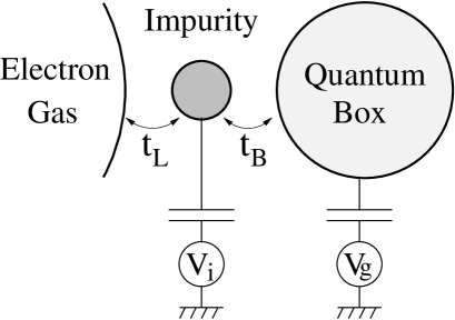
Figure 1: Schematic sketch of the physical setting. A quantum box and a metallic lead are each coupled by tunneling to an intermediate impurity level. The charge inside the quantum box is tuned by varying the gate voltage $V_{g}$, while the energy of the level is controlled by varying the gate voltage $V_{i}$.

II Coulomb blockade with resonant tunneling

The physical setting under consideration is shown schematically in Fig. 1. It consists of a metallic lead and a quantum box, each coupled by tunneling to an impurity placed in between the lead and box. The impurity is assumed to have just a single energy level $\epsilon_{d}$ in the relevant energy range, described by the two creation operators $d^{\dagger}_{\uparrow}$ and $d^{\dagger}_{\downarrow}$. The quantum box is characterized by the single-particle dispersion $\epsilon_{kB}$, and by the charging energy $E_{C}=e^{2}/2C$. Here $C$ is the capacitance of the box. The mean level spacing inside the box is assumed to be considerably smaller than all other energy scales in the problem, such that a continuum-limit description can be used. The charge inside the box is controlled by varying the gate voltage $V_{g}$, which determines the electrostatic potential inside the box. We parameterize the latter by the dimensionless number $N=C_{g}V_{g}/e$, where $C_{g}$ is the capacitance of the gate, and $-e$ is the electron charge.

Modeling the lead by a noninteracting band with dispersion $\epsilon_{kL}$, the Hamiltonian of the system is given by

$${\cal H} = \sum_{\alpha=L,B}\sum_{k,\sigma}\epsilon_{k\alpha}c^{\dagger}_{k\alpha\sigma}c_{k\alpha\sigma}+\epsilon_{d}\sum_{\sigma}d^{\dagger}_{\sigma}d_{\sigma}$$

$$+ \sum_{k,\sigma\alpha}t_{k\alpha}\left\{c^{\dagger}_{k\alpha\sigma}d_{\sigma}+{\rm H.c.}\right\}+E_{C}(\hat{n}-N)^{2},$$

where $c^{\dagger}_{kL\sigma}$ ($c^{\dagger}_{kB\sigma}$) creates an electron with spin projection $\sigma$ in the lead (box); $t_{kL}$ ($t_{kB}$) are the matrix elements for tunneling between the impurity and the lead (box); and

$$\hat{n}=\sum_{k,\sigma}\left[c^{\dagger}_{kB\sigma}c_{kB\sigma}-\theta(-\epsilon_{kB})\right]$$ (2)

measures the number of excess electrons in the box. Here and throughout the paper we set the chemical potential as our reference energy, namely, all single-particle energies are measured relative to the chemical potential. For an interacting level, Eq. (II) is supplemented by the on-site repulsion term

$${\cal H}_{U}=U\hat{n}_{d\uparrow}\hat{n}_{d\downarrow},$$ (3)

where $\hat{n}_{d\sigma}=d^{\dagger}_{\sigma}d_{\sigma}$ are the number operators on the level.

The Hamiltonian of Eq. (II) features two basic energy scales,

$$\Gamma_{L} = \pi\sum_{k}t_{kL}^{2}\delta(\epsilon_{kL}),$$ (4)

$$\Gamma_{B} = \pi\sum_{k}t_{kB}^{2}\delta(\epsilon_{kB}),$$ (5)

corresponding to half the tunneling rates from the impurity to the lead and to the box, respectively. As shown by Gramespacher and Matveev, GM00 for $\Gamma_{L},\Gamma_{B}\ll E_{C}$ there is a nearly perfect Coulomb staircase, even if the transmission coefficient through the impurity is one at the Fermi energy. The shape of the sharp steps near half-integer values of $N$ was left unresolved in Ref. GM00, , which is the objective of the present paper. To this end, we focus hereafter on $N=n+\frac{1}{2}+\delta N$, where $n$ is an integer and $|\delta N|\ll 1$. This range in $N$ corresponds to the step separating the two charge plateaus with $n$ and $n+1$ excess electrons in the box.

For temperatures well below the charging energy, $k_{B}T\ll E_{C}$, only the $n$ and $n+1$ charge configurations are thermally accessible in the box. Hence one can remove all excited charge configurations by projecting the Hamiltonian of Eq. (II) onto the $n$ and $n+1$ subspaces. Following Matveev, Matveev91 a spin-$\frac{1}{2}$ isospin operator $\vec{S}$ is introduced to label the two available charge configurations: $S_{z}=1/2$ for the $n+1$ subspace, and $S_{z}=-1/2$ for the $n$ subspace. The raising and lowering operators, $S^{\pm}=S_{x}\pm iS_{y}$, describe then transitions between the $n$ and $n+1$ subspaces, corresponding to the addition or removal of a box electron. Hence the Hamiltonian of Eq. (II) is converted to ${\cal H}={\cal H}_{L}+{\cal H}_{B}+{\cal H}_{tun}$, where

$${\cal H}_{L} = \sum_{k,\sigma}\epsilon_{kL}c^{\dagger}_{kL\sigma}c_{kL\sigma}+\epsilon_{d}\sum_{\sigma}d^{\dagger}_{\sigma}d_{\sigma}$$

$$+ \sum_{k,\sigma}t_{kL}\left\{c^{\dagger}_{kL\sigma}d_{\sigma}+{\rm H.c.}\right\}$$

describes the coupled lead and impurity,

$${\cal H}_{B}=\sum_{k,\sigma}\epsilon_{kB}c^{\dagger}_{kB\sigma}c_{kB\sigma}-eV_{B}S_{z}$$ (7)

with $eV_{B}=2E_{C}\delta N$ describes the isolated box, and

$${\cal H}_{tun}=\sum_{k,\sigma}t_{kB}\left\{c^{\dagger}_{kB\sigma}d_{\sigma}S^{+}+{\rm H.c.}\right\}$$ (8)

describes tunneling between the impurity and the box. For an interacting level, the above Hamiltonian is supplemented by the on-site interaction term of Eq. (3).

Equations (II)–(8) are a straightforward generalization of Matveev’s original mapping for a weak tunnel barrier. Matveev91 As in the case of a weak tunnel barrier, the average excess charge in the box takes the form

$$\langle Q\rangle=-e\left(n+\frac{1}{2}\right)-e\langle S_{z}\rangle,$$ (9)

while the capacitance of the junction,

$$C(V_{B},T)=-\partial\langle Q\rangle/\partial V_{B},$$ (10)

is proportional to the isospin susceptibility. The connection between the Hamiltonian of Eqs. (II)–(8) and the two-channel Kondo model is less transparent than for a weak tunnel barrier, since the tunneling Hamiltonian ${\cal H}_{tun}$ involves the localized $d^{\dagger}_{\sigma}$ degrees of freedom. As we show in the following section, one can still relate the Hamiltonian of Eqs. (II)–(8) to the two-channel Kondo model, by first diagonalizing the quadratic Hamiltonian term ${\cal H}_{L}$. This gives rise to a new variant of the planner two-channel Kondo Hamiltonian, in which the spin-up and the spin-down conduction electrons have two distinct bandwidths.

III Relation to the two-channel Kondo Hamiltonian

Much of the underlying physics of the Hamiltonian of Eqs. (II)–(8) can be understood by converting to a single-particle basis that diagonalizes the quadratic Hamiltonian term ${\cal H}_{L}$. The objective of this section is to construct such a basis. In doing so we assume that the level $\epsilon_{d}$ lies well within the band (i.e., no bound state is formed), and neglect for simplicity all $k$-dependence of the tunneling matrix elements $t_{kL}$ and $t_{kB}$. The latter are taken for convenience to be real and positive.

A convenient representation of the eigen modes of ${\cal H}_{L}$ involves the $d$-electron Green function

$$G(z)=\left[z-\epsilon_{d}-t_{L}^{2}\sum_{k}\frac{1}{z-\epsilon_{kL}}\right]^{-1},$$ (11)

along with the associated phases

$$\phi_{k}={\rm arg}\left\{G(\epsilon_{kL}-i\eta)\right\}.$$ (12)

Here $\eta$ is a positive infinitesimal. Introducing the properly normalized fermion operators

$$\psi^{\dagger}_{kL\sigma}= e^{i\phi_{k}}c^{\dagger}_{kL\sigma}+t_{L}|G(\epsilon_{kL}+i\eta)|$$

$$\times\left[d^{\dagger}_{\sigma}+t_{L}\sum_{k^{\prime}}\frac{1}{\epsilon_{kL}-\epsilon_{k^{\prime}L}+i\eta}c^{\dagger}_{k^{\prime}L\sigma}\right],$$

the Hamiltonian term ${\cal H}_{L}$ acquires the diagonal form

$${\cal H}_{L}=\sum_{k,\sigma}\epsilon_{kL}\psi^{\dagger}_{kL\sigma}\psi_{kL\sigma},$$ (14)

while the $d^{\dagger}_{\sigma}$ operators are expanded as

$$d^{\dagger}_{\sigma}=t_{L}\sum_{k}|G(\epsilon_{kL}+i\eta)|\psi^{\dagger}_{kL\sigma}.$$ (15)

Further converting to the constant-energy-shell operators

$$a^{\dagger}_{\epsilon L\sigma} = \frac{1}{\sqrt{\rho_{L}(\epsilon)}}\sum_{k}\delta(\epsilon-\epsilon_{kL})\psi^{\dagger}_{kL\sigma},$$ (16)

$$a^{\dagger}_{\epsilon B\sigma} = \frac{1}{\sqrt{\rho_{B}(\epsilon)}}\sum_{k}\delta(\epsilon-\epsilon_{kB})c^{\dagger}_{kB\sigma}$$ (17)

[here $\rho_{L}(\epsilon)$ and $\rho_{B}(\epsilon)$ are the underlying lead and box density of states, respectively], the full Hamiltonian reads

$${\cal H} = \sum_{\alpha=L,B}\sum_{\sigma}\int\epsilon a^{\dagger}_{\epsilon\alpha\sigma}a_{\epsilon\alpha\sigma}d\epsilon-eV_{B}S_{z}$$

$$+ \frac{1}{2}\sum_{\sigma}\int d\epsilon\int d\epsilon^{\prime}J(\epsilon,\epsilon^{\prime})\left\{a^{\dagger}_{\epsilon B\sigma}a_{\epsilon^{\prime}L\sigma}S^{+}+{\rm H.c.}\right\}.$$

Here, $eV_{B}$ is equal to $2E_{C}\delta N$; the energy-dependent coupling $J(\epsilon,\epsilon^{\prime})$ is given by

$$J(\epsilon,\epsilon^{\prime})=2t_{L}t_{B}\sqrt{\rho_{B}(\epsilon)\rho_{L}(\epsilon^{\prime})}|G(\epsilon^{\prime}+i\eta)|;$$ (19)

and the single-particle operators $a_{\epsilon\alpha\sigma}$ obey canonical anticommutation relations:

$$\left\{a_{\epsilon\alpha\sigma},a^{\dagger}_{\epsilon^{\prime}\alpha^{\prime}\sigma^{\prime}}\right\}=\delta(\epsilon-\epsilon^{\prime})\delta_{\alpha\alpha^{\prime}}\delta_{\sigma\sigma^{\prime}}.$$ (20)

Note that we have omitted in Eq. (III) all those conduction-electron channels in both ${\cal H}_{L}$ and ${\cal H}_{B}$ that decouple from the tunneling term ${\cal H}_{tun}$.

Equation (III) should be compared with the corresponding constant-energy-shell representation of the planner two-channel Kondo model with a local magnetic field. In the latter case, the indices $L$ and $B$ are replaced with spin-up and spin-down labels, $eV_{B}$ corresponds to the local magnetic field, and $\sigma$ acts as the channel index. More significantly, $J(\epsilon,\epsilon^{\prime})$ of Eq. (19) is replaced with $J_{2CK}(\epsilon,\epsilon^{\prime})=\sqrt{\rho(\epsilon)\rho(\epsilon^{\prime})}J_{\perp}$, where $J_{\perp}$ is the transverse Kondo coupling, and $\rho(\epsilon)$ is the joint density of states (DOS) of the spin-up and spin-down conduction electrons. Thus, identifying the lead and box indices $L$ and $B$ with isospin-up and isospin-down labels, Matveev91 Eq. (III) coincides with the planner two-channel Kondo Hamiltonian modulo one crucial difference: the effective DOS for the isospin-up and isospin-down conduction electrons are markedly different in Eq. (III). While the isospin-down DOS is equal to $\rho_{B}(\epsilon)$, the effective isospin-up DOS is given by the spectral part of $G(z)$: comment_on_rho_L^eff

$$\rho_{L}^{\rm eff}(\epsilon)=-\frac{1}{\pi}{\rm Im}\left\{G(\epsilon+i\eta)\right\}=t^{2}_{L}\rho_{L}(\epsilon)|G(\epsilon+i\eta)|^{2}.$$ (21)

In the wide-band limit, and for $\epsilon$ well within the band, Eq. (21) reduces to the Lorentzian form

$$\rho_{L}^{\rm eff}(\epsilon)=\frac{1}{\pi}\frac{\Gamma_{L}}{(\epsilon-\epsilon_{d})^{2}+\Gamma_{L}^{2}}.$$ (22)

Hence the effective bandwidth for the isospin-up electrons is equal to $\Gamma_{L}$, i.e., notably smaller than the isospin-down bandwidth $D$. comment_on_D Such a large separation of bandwidths for the isospin-up and isospin-down conduction electrons has no analog in the conventional two-channel Kondo Hamiltonian, where the two spin orientations are identical for a zero magnetic field. Moreover, $\rho_{L}^{\rm eff}(\epsilon)$ is centered about $\epsilon_{d}$, which corresponds for $|\epsilon_{d}|\gg\Gamma_{L}$ either to a nearly filled band ($\epsilon_{d}<0$) or to a nearly empty band ($\epsilon_{d}>0$). Below we explore in detail the consequences of these deviations from the conventional two-channel Kondo Hamiltonian, but first let us give some heuristic arguments for the expected low-energy physics in the case where $\epsilon_{d}=0$.

As is well known, the low-energy physics of the planner two-channel Kondo model is governed by the dimensionless coupling $\rho_{0}J_{\perp}$, where $\rho_{0}=\rho(0)$ is the conduction-electron DOS at the Fermi energy. By analogy with the two-channel Kondo Hamiltonian,

$$J(0,0)=\frac{2}{\pi}\sqrt{\frac{\Gamma_{L}\Gamma_{B}}{\epsilon_{d}^{2}+\Gamma_{L}^{2}}}$$ (23)

plays the role of $\rho_{0}J_{\perp}$ in the Hamiltonian of Eq. (III). Specifically, for a level at resonance with the Fermi energy, i.e., $\epsilon_{d}=0$, Eq. (23) is equal to $(2/\pi)\sqrt{\Gamma_{B}/\Gamma_{L}}$.

To the extent that the Hamiltonian of Eq. (III) still flows for $\epsilon_{d}=0$ and $V_{B}=0$ to the intermediate-coupling fixed point of the two-channel Kondo effect, different qualitative behaviors are expected of the Kondo temperature $T_{K}$ in each of the limits $\Gamma_{B}\ll\Gamma_{L}$ and $\Gamma_{L}\ll\Gamma_{B}$. For $\Gamma_{B}\ll\Gamma_{L}$, the bare spin-exchange interaction is weak. Hence $T_{K}$ should be exponentially small in $\sqrt{\Gamma_{L}/\Gamma_{B}}\sim 1/J(0,0)$. In the opposite limit, $\Gamma_{L}\ll\Gamma_{B}$, the dimensionless coupling $J(\epsilon,\epsilon^{\prime})$ crosses over from weak to strong coupling as $|\epsilon^{\prime}|$ is reduced below $k_{B}T_{x}\sim\sqrt{\Gamma_{L}\Gamma_{B}}$. Anticipating a relation between $T_{K}$ and $T_{x}$, one expects then a Kondo temperature that is neither exponentially small in $1/\sqrt{\Gamma_{L}}$, nor in $1/\sqrt{\Gamma_{B}}$.

Obviously, the above picture relies heavily on the conjecture that the Hamiltonian of Eq. (III) flows for $\epsilon_{d}=0$ and $V_{B}=0$ to the intermediate-coupling fixed point of the two-channel Kondo effect, and on intuition borrowed from the conventional two-channel Kondo Hamiltonian. Although neither assumption is justified a priori, this tentative picture is shown below to be surprisingly accurate.

IV Weak coupling

We begin our discussion with the limit of weak coupling, $J(0,0)\ll 1$, for which an analytical treatment is possible. Specifically, we employ a perturbative scaling approach based on Anderson’s poor-man’s scaling, Anderson70 to study two generic cases: (i) $\epsilon_{d}=0$ and $\Gamma_{B}\ll\Gamma_{L}$, corresponding to an impurity level at resonance with the Fermi energy; and (ii) $|\epsilon_{d}|\gg\Gamma_{B},\Gamma_{L}$, corresponding to an impurity level off resonance with the Fermi energy. Throughout this paper we assume a symmetric rectangular form for the underlying lead and box density of states, with a single joint bandwidth $D$. comment_on_D The latter is taken to be much larger than $|\epsilon_{d}|,\Gamma_{B}$, and $\Gamma_{L}$, such that $\rho_{L}^{\rm eff}(\epsilon)=t^{2}_{L}\rho_{L}(\epsilon)|G(\epsilon+i\eta)|^{2}$ has the Lorentzian form of Eq. (22).

IV.1 Level at resonance with the Fermi energy

Consider first the case where $\epsilon_{d}=0$ and $\Gamma_{B}\ll\Gamma_{L}$. For $\epsilon_{d}=0$, the Lorentzian DOS $\rho_{L}^{\rm eff}(\epsilon)$ is centered about the Fermi energy. To proceed with our analytical treatment, it is convenient to replace $\rho_{L}^{\rm eff}(\epsilon)$ with a symmetric rectangular DOS that preserves both the height of $\rho_{L}^{\rm eff}(\epsilon)$ at the Fermi energy, and its total integrated weight:

$$\rho_{L}^{\rm eff}(\epsilon)\longrightarrow\frac{1}{\pi\Gamma_{L}}\theta\left(\frac{\pi\Gamma_{L}}{2}-|\epsilon|\right).$$ (24)

With this modification, and using the relation $J(\epsilon,\epsilon^{\prime})=2t_{B}\sqrt{\rho_{B}(\epsilon)\rho_{L}^{\rm eff}(\epsilon^{\prime})}$, the Hamiltonian of Eq. (III) becomes

$${\cal H} = \sum_{\sigma}\int_{-D_{L}}^{D_{L}}\epsilon a^{\dagger}_{\epsilon L\sigma}a_{\epsilon L\sigma}d\epsilon+\sum_{\sigma}\int_{-D}^{D}\epsilon a^{\dagger}_{\epsilon B\sigma}a_{\epsilon B\sigma}d\epsilon$$ (25)

$$+ \frac{\tilde{J}_{\perp}}{2}\sum_{\sigma}\int_{-D}^{D}\!\!d\epsilon\int_{-D_{L}}^{D_{L}}\!\!d\epsilon^{\prime}\!\left\{a^{\dagger}_{\epsilon B\sigma}a_{\epsilon^{\prime}L\sigma}S^{+}+{\rm H.c.}\right\}$$

$$- eV_{B}S_{z},$$

where $\tilde{J}_{\perp}=(2/\pi)\sqrt{\Gamma_{B}/\Gamma_{L}}\ll 1$ is the effective isospin exchange interaction, and $D_{L}$ is equal to $\pi\Gamma_{L}/2$. Hereafter we assume that $e|V_{B}|\ll D_{L}$.

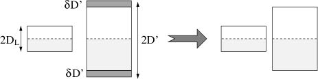
Figure 2: The basic iterative step in the perturbative scaling procedure, for $D>D_{L}$. Suppose that the isospin-down ($B$) bandwidth has already been lowered from its initial value $D$ to some smaller value $D>D^{\prime}>D_{L}$. The bandwidth $D^{\prime}$ is then further reduced to $D^{\prime}-\delta D^{\prime}$ using poor-man’s scaling, while maintaining the isospin-up ($L$) bandwidth at $D_{L}$. This procedure is repeated until $D^{\prime}$ coincides with $D_{L}$, leaving just a single common bandwidth for the two isospin orientations.

To cope with the different bandwidths in Eq. (25), we proceed with perturbative scaling. Using poor-man’s scaling, Anderson70 we successively reduce the larger bandwidth from $D$ down to $D_{L}$, mapping thereby the Hamiltonian of Eq. (25) onto an effective low-energy Hamiltonian with a single joint bandwidth $D_{L}$. The basic iterative step in this procedure is illustrated in Fig. 2. Suppose that the isospin-down ($B$) bandwidth has already been lowered from its initial value $D$ to some value $D^{\prime}=De^{-l}$, $0<l<\ln(D/D_{L})$. Further reducing the bandwidth to $D^{\prime}(1-\delta l)$ produces a renormalization to a new interaction term not present in the original Hamiltonian:

$$\lambda\sum_{\sigma}\int_{-D_{L}}^{D_{L}}d\epsilon\int_{-D_{L}}^{D_{L}}d\epsilon^{\prime}:\!a^{\dagger}_{\epsilon L\sigma}a_{\epsilon^{\prime}L\sigma}\!:S_{z}.$$ (26)

Here $:\!a^{\dagger}_{\epsilon L\sigma}a_{\epsilon^{\prime}L\sigma}\!:=a^{\dagger}_{\epsilon L\sigma}a_{\epsilon^{\prime}L\sigma}\!-\theta(-\epsilon)\delta(\epsilon-\epsilon^{\prime})$ stands for normal ordering with respect to the filled isospin-down ($L$) Fermi sea. Explicitly, $\lambda$ renormalizes according to the scaling equation

$$\frac{d\lambda}{dl}=\frac{1}{2}\tilde{J}_{\perp}^{2},$$ (27)

where $\tilde{J}_{\perp}=(2/\pi)\sqrt{\Gamma_{B}/\Gamma_{L}}$ is the bare isospin-exchange coupling in Eq. (25). Indeed, the $\tilde{J}_{\perp}$ interaction term remains unchanged in Eq. (25) throughout this procedure, apart from the reduced integration range over $\epsilon$. For a nonzero $\epsilon_{d}$, there is an additional renormalization of the “magnetic” field $eV_{B}$, discussed below.

Upon reducing $D$ down to $D_{L}$, the new coupling $\lambda$ grows from zero to $\frac{1}{2}\tilde{J}_{\perp}^{2}\ln(D/D_{L})$. Thus, for $D^{\prime}=D_{L}$ one arrives at the effective Hamiltonian

$${\cal H} = \sum_{\sigma}\sum_{\alpha=L,B}\int_{-D_{L}}^{D_{L}}\epsilon a^{\dagger}_{\epsilon\alpha\sigma}a_{\epsilon\alpha\sigma}d\epsilon-eV_{B}S_{z}$$

$$+ \frac{\tilde{J}_{\perp}}{2}\sum_{\sigma}\int_{-D_{L}}^{D_{L}}\!\!d\epsilon\int_{-D_{L}}^{D_{L}}\!\!d\epsilon^{\prime}\left\{a^{\dagger}_{\epsilon B\sigma}a_{\epsilon^{\prime}L\sigma}S^{+}+{\rm H.c.}\right\}$$

$$+ \frac{\tilde{J}_{z}}{2}\sum_{\sigma}\int_{-D_{L}}^{D_{L}}\!\!d\epsilon\int_{-D_{L}}^{D_{L}}\!\!d\epsilon^{\prime}\left\{a^{\dagger}_{\epsilon L\sigma}a_{\epsilon^{\prime}L\sigma}-a^{\dagger}_{\epsilon B\sigma}a_{\epsilon^{\prime}B\sigma}\right\}S_{z}$$

$$+ \tilde{V}\sum_{\sigma,\alpha}\int_{-D_{L}}^{D_{L}}\!\!d\epsilon\int_{-D_{L}}^{D_{L}}\!\!d\epsilon^{\prime}:\!a^{\dagger}_{\epsilon\alpha\sigma}a_{\epsilon^{\prime}\alpha\sigma}\!:S_{z},$$

where $\tilde{J}_{z}=2\tilde{V}=\frac{1}{2}\tilde{J}_{\perp}^{2}\ln(D/D_{L})$. Here we have separated the interaction term of Eq. (27) into a longitudinal isospin-exchange interaction $\tilde{J}_{z}$, and a $\tilde{V}$ term.

Apart from the extra $\tilde{V}$ term, Eq. (IV.1) has the form of a conventional two-channel Kondo Hamiltonian with an anisotropic spin-exchange interaction. As in the case of a weak tunnel barrier, Matveev91 the indices $L$ and $B$ are identified in such a mapping with isospin-up and isospin-down labels, while the physical spin $\sigma$ serves as a conserved channel index. Contrary to the case of a weak tunnel barrier, though, the Hamiltonian of Eq. (IV.1) contains a longitudinal Kondo coupling $\tilde{J}_{z}$, which can be either smaller or larger than $\tilde{J}_{\perp}$. For $\frac{1}{2}\tilde{J}_{\perp}\ln(D/D_{L})\ll 1$ [i.e., $(1/\pi)\sqrt{\Gamma_{B}/\Gamma_{L}}\ln(D/\Gamma_{L})\ll 1$] one has $\tilde{J}_{z}\ll\tilde{J}_{\perp}$, while for $\frac{1}{2}\tilde{J}_{\perp}\ln(D/D_{L})\gg 1$ the order is reversed. It should be emphasized, however, that $\Gamma_{L}$ (and thus also $\Gamma_{B}\ll\Gamma_{L}$) must be exponentially small in this range in order for $\tilde{J}_{z}$ to become comparable to $\tilde{J}_{\perp}$.

It is straightforward to verify using perturbative renormalization-group (RG) methods that the $\tilde{V}$ term acts much in the same way as ordinary potential scattering: It is a marginal operator, that does not affect (at least not to second order) the Kondo couplings’ flow toward strong coupling. For $V_{B}=0$, the Hamiltonian of Eq. (IV.1) thus flows to the non-Fermi-liquid fixed point of the two-channel Kondo effect, as in the case of a weak tunnel barrier. Matveev91 The corresponding Kondo temperature can be extracted in turn from known results for the anisotropic two-channel Kondo model. In particular, for $\tilde{J}_{z}\ll\tilde{J}_{\perp}$ this can be done quite elegantly by iterating the standard RG equations backwards (i.e., increasing the bandwidth $D_{L}$), to obtain a planner two-channel Kondo Hamiltonian with a bandwidth $D^{\ast}>D_{L}$ and a transverse Kondo coupling $\tilde{J}^{\ast}_{\perp}$, that shares the same $T_{K}$. To leading order in $\tilde{J}_{\perp}$ and $\tilde{J}_{z}/\tilde{J}_{\perp}$ one obtains

$$D^{\ast}=\sqrt{D_{L}D}\;,\;\;\;\;\tilde{J}^{\ast}_{\perp}=\tilde{J}_{\perp}=\frac{2}{\pi}\sqrt{\frac{\Gamma_{B}}{\Gamma_{L}}}.$$ (29)

Substituting the above parameters into the expression for the Kondo temperature of the planner two-channel Kondo Hamiltonian T_K_planner_model yields

$$k_{B}T_{K}=\sqrt{\Gamma_{B}D}\ \exp\left[-\frac{\pi^{2}}{4}\sqrt{\frac{\Gamma_{L}}{\Gamma_{B}}}\right].$$ (30)

Here, as usual, $T_{K}$ is given up to a factor of order unity, which depends both on the precise definition of the Kondo temperature, and on the actual Lorentzian form of $\rho_{L}^{\rm eff}(\epsilon)$.

Two comments should be made about Eqs. (29)–(30). First, as seen in Eq. (29), the effective bandwidth for $\tilde{J}_{z}\ll\tilde{J}_{\perp}$ is neither $D$ nor $D_{L}$, but rather their geometric average, $D^{\ast}$. Therefore, the effect of the narrow resonance that forms on the level is to reduce the effective bandwidth in the problem. Second, similar to the case of a weak tunnel barrier, Matveev91 the exponential dependence in Eq. (30) can be recast in the form $\exp\!\left[-\pi^{2}/2\sqrt{\cal T}\right]$, where ${\cal T}=4\Gamma_{B}/\Gamma_{L}$ is the transmission coefficient through the impurity at the Fermi energy for $\Gamma_{B}\ll\Gamma_{L}$. Hence a resonant level with $\epsilon_{d}=0$ and $\Gamma_{B}\ll\Gamma_{L}$ acts similar to a poorly conducting tunnel barrier with a transmission coefficient equal to ${\cal T}=4\Gamma_{B}/\Gamma_{L}$.

IV.2 Level off resonance with the Fermi energy

Next we consider a level off resonance with the Fermi energy, namely, $|\epsilon_{d}|\gg\Gamma_{L},\Gamma_{B}$. As noted by Gramespacher and Matveev, GM00 tunneling into and out of the quantum box are no longer equivalent for $\epsilon_{d}\neq 0$. Depending on the sign of $\epsilon_{d}$, this has the effect of either pushing down or pulling up the charge plateaus. Using perturbative scaling we show below that a nonzero $\epsilon_{d}$ also shifts the position of the degeneracy point, maintaining the two-channel Kondo effect at the shifted position of degeneracy point.

To devise a perturbative scaling treatment of the case $|\epsilon_{d}|\gg\Gamma_{L},\Gamma_{B}$, one can use either the original Hamiltonian of Eqs. (II)–(8), or the equivalent representation of Eq. (III). In the former representation, one first reduces the bandwidth from its bare value $D$ to an effective bandwidth of the order of $|\epsilon_{d}|$, and then performs a Schrieffer-Wolff transformation SW66 to eliminate the charge fluctuations on the level. These two steps enter the representation of Eq. (III) in a unified fashion through the energy dependence of the coupling $J(\epsilon,\epsilon^{\prime})$, which is sharply peaked as a function of $\epsilon^{\prime}$ at $\epsilon_{d}$.

We have carried out both the perturbative scaling approach based on the Hamiltonian representation of Eqs. (II)–(8), and the scheme based on the Hamiltonian representation of Eq. (III). Both procedures give the same results to leading order in $\Gamma_{L}/|\epsilon_{d}|$ and $\Gamma_{B}/|\epsilon_{d}|$ (note that the Schrieffer-Wolff transformation is designed to capture only the leading order in these parameters). For the sake of consistency with the analysis of the previous subsection, we present below the approach based on the Hamiltonian representation of Eq. (III).

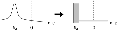
Figure 3: Illustration of the density-of-states substitution $\rho^{\rm eff}_{L}(\epsilon)\to\bar{\rho}_{\rm eff}(\epsilon)$, for $\epsilon_{d}<0$. For $|\epsilon_{d}|\gg\Gamma_{L}$, the Lorentzian $\rho_{L}^{\rm eff}(\epsilon)$ has two prominent features: a narrow peak of width $\sim\Gamma_{L}$ and weight $w\approx 1$ centered about $\epsilon_{d}$, and a shallow tail that crosses the Fermi energy. Each of these features is conveniently mimicked within $\bar{\rho}_{\rm eff}(\epsilon)$ by a rectangular structure, one narrow and sharp centered about $\epsilon_{d}$, and the other broad and shallow centered about the Fermi energy.

Similar to the case of a level at resonance with the Fermi energy, it is convenient to replace $\rho_{L}^{\rm eff}(\epsilon)$ with a simplified density of states that captures the essential features of $\rho_{L}^{\rm eff}(\epsilon)$, and allows for an analytical treatment of the problem. Specifically, $\rho_{L}^{\rm eff}(\epsilon)$ has two prominent features: a narrow resonance of width $\sim\Gamma_{L}$ and weight $1-{\cal O}\left(\Gamma_{L}/|\epsilon_{d}|\right)$ centered about $\epsilon=\epsilon_{d}$, and a shallow tail that crosses the Fermi energy and provides the low-energy excitations for the development of the Kondo effect. To mimic these two features, we replace $\rho_{L}^{\rm eff}(\epsilon)$ with the double-rectangular density of states illustrated in Fig. 3:

$$\bar{\rho}_{\rm eff}(\epsilon)=\frac{w}{2D_{L}}\theta\left(D_{L}-|\epsilon-\epsilon_{d}|\right)+\frac{\Gamma_{L}}{\pi\epsilon_{d}^{2}}\theta\left(D_{m}-|\epsilon|\right).$$ (31)

Here $D_{m}=|\epsilon_{d}|-D_{L}$ is a crude measure of the extent of the tail that crosses the Fermi energy, $D_{L}=\pi\Gamma_{L}/2$ corresponds to half the width of the resonance at $\epsilon=\epsilon_{d}$, and $w=1-2\Gamma_{L}D_{m}/(\pi\epsilon_{d}^{2})\approx 1$ is the effective weight of the resonance.

Obviously, there is some arbitrariness in our choice of $\bar{\rho}_{\rm eff}(\epsilon)$, which differs in details from $\rho_{L}^{\rm eff}(\epsilon)$. In particular, the extent of the tail that crosses the Fermi energy is somewhat exaggerated, while the opposite tail (the one extending away from the Fermi energy) is absent. Nevertheless, this choice of $\bar{\rho}_{\rm eff}(\epsilon)$ is compatible with the approximations made in the Schrieffer-Wolff transformation, and gives the correct results to leading order in $\Gamma_{L}/|\epsilon_{d}|$ and $\Gamma_{B}/|\epsilon_{d}|$. Substituting $\bar{\rho}_{\rm eff}(\epsilon)$ in for $\rho_{L}^{\rm eff}(\epsilon)$, the Hamiltonian of Eq. (III) becomes

$${\cal H} = \sum_{\sigma}\int_{-D_{p}}^{D_{p}}\epsilon a^{\dagger}_{\epsilon L\sigma}a_{\epsilon L\sigma}d\epsilon-eV_{B}S_{z}$$

$$+ \sum_{\sigma}\int_{-D}^{D}\epsilon a^{\dagger}_{\epsilon B\sigma}a_{\epsilon B\sigma}d\epsilon$$

$$+ \sqrt{\frac{\Gamma_{B}}{\pi}}\sum_{\sigma}\int_{-D}^{D}\!\!d\epsilon\int_{-D_{p}}^{D_{p}}\!\!d\epsilon^{\prime}\!\sqrt{\bar{\rho}_{\rm eff}(\epsilon^{\prime})}$$

$$\;\;\;\;\;\;\;\;\;\;\;\;\;\;\;\;\;\;\;\;\;\;\times\left\{a^{\dagger}_{\epsilon B\sigma}a_{\epsilon^{\prime}L\sigma}S^{+}+{\rm H.c.}\right\},$$

where $D_{p}=|\epsilon_{d}|+D_{L}$. Hereafter we assume that $e|V_{B}|\ll|\epsilon_{d}|$.

To treat the Hamiltonian of Eq. (IV.2), we proceed with perturbative scaling. This is done in two stages. First the larger bandwidth is successively reduced from its bare value $D$ down to $D_{p}$, leaving just a single common bandwidth for the two conduction seas. This common bandwidth is subsequently reduced from $D_{p}$ down to $D_{m}$.

The first step in the above scheme is similar to the one implemented in the previous subsection, when treating a level at resonance with the Fermi energy. There are, however, three important modifications. First, the new interaction term generated upon scaling has the form

$$\lambda\sum_{\sigma}\int_{-D_{p}}^{D_{p}}d\epsilon\int_{-D_{p}}^{D_{p}}d\epsilon^{\prime}\sqrt{\bar{\rho}_{\rm eff}(\epsilon)\bar{\rho}_{\rm eff}(\epsilon^{\prime})}:\!a^{\dagger}_{\epsilon L\sigma}a_{\epsilon^{\prime}L\sigma}\!:S_{z},$$ (33)

which differs from Eq. (26) in the extra square roots of $\bar{\rho}_{\rm eff}$ that enter the integrand. Second, the coupling $\lambda$ renormalizes according to the scaling equation

$$\frac{d\lambda}{dl}=\frac{2\Gamma_{B}}{\pi},$$ (34)

which likewise differs from Eq. (27). Lastly, the voltage $V_{B}$ is renormalized at $T=0$ according to

$$\frac{d\tilde{V}_{B}}{dl}={\rm sign}(\epsilon_{d})\frac{2\Gamma_{B}}{\pi}\frac{1}{1+e^{l}|\epsilon_{d}|/D}.$$ (35)

Here we have distinguished the running parameter $\tilde{V}_{B}$ from its bare value $V_{B}$, and omitted higher order corrections in $\Gamma_{L}/|\epsilon_{d}|$. Upon reducing the larger bandwidth from $D$ down to $D_{p}$, the coupling $\lambda$ thus grows from zero to $(2\Gamma_{B}/\pi)\ln(D/D_{p})$, while $e\tilde{V}_{B}$ evolves from $eV_{B}$ to $eV_{B}+{\rm sign}(\epsilon_{d})(2\Gamma_{B}/\pi)\ln\left[\frac{1}{2}+\frac{D}{2|\epsilon_{d}|}\right]$.

Since we are interested in $|\epsilon_{d}|\gg\Gamma_{L}$, one can proceed to eliminate all excitations in the energy range $D_{p}>\epsilon>D_{m}$ in one step, by working with a finite $\delta l=2D_{L}/D_{p}\ll 1$. Within the Hamiltonian representation of Eqs. (II)–(8), this step is equivalent to carrying out the Schrieffer-Wolff transformation. At the end of this procedure one arrives at an effective Hamiltonian of the form of Eq. (IV.1), where $D_{L}$ is replaced with $D_{m}$, plus two additional potential-scattering terms:

$$\tilde{V}_{\pm}\sum_{\sigma}\int_{-D_{m}}^{D_{m}}\!\!d\epsilon\int_{-D_{m}}^{D_{m}}\!\!d\epsilon^{\prime}\left\{:\!a^{\dagger}_{\epsilon L\sigma}a_{\epsilon^{\prime}L\sigma}\!:\pm:\!a^{\dagger}_{\epsilon B\sigma}a_{\epsilon^{\prime}B\sigma}\!:\right\}.$$ (36)

The effective coupling constants entering the resulting Hamiltonian are quite different, however, from those in Eq. (IV.1), and are given by

$$\tilde{J}_{\perp}=\frac{2}{\pi}\frac{\sqrt{\Gamma_{L}\Gamma_{B}}}{|\epsilon_{d}|},$$ (37)

$$\tilde{J}_{z}=\frac{1}{\pi}\frac{\Gamma_{B}}{|\epsilon_{d}|},$$ (38)

$$\tilde{V}=-\frac{1}{2\pi}\frac{\Gamma_{B}}{|\epsilon_{d}|},$$ (39)

$$\tilde{V}_{+}=-\frac{1}{4\pi}\frac{\Gamma_{B}}{|\epsilon_{d}|}{\rm sign}(\epsilon_{d}),$$ (40)

$$\tilde{V}_{-}=\frac{1}{4\pi}\frac{\Gamma_{B}}{|\epsilon_{d}|}{\rm sign}(\epsilon_{d}),$$ (41)

Here we have omitted corrections that are smaller by factors of $\Gamma_{\alpha}/|\epsilon_{d}|$ or $(\Gamma_{\alpha}/\pi|\epsilon_{d}|)\ln(D/|\epsilon_{d}|)$ than the leading-order terms. In addition, the voltage $V_{B}$ is renormalized at $T=0$ according to

$$eV_{B}\to e\tilde{V}_{B}=eV_{B}+{\rm sign}(\epsilon_{d})\frac{2\Gamma_{B}}{\pi}\ln\left(1+\frac{D}{|\epsilon_{d}|}\right).$$ (42)

It is straightforward to verify using either poor-man’s scaling or bosonization (in combination with a canonical transformation) that the $V_{\pm}$ terms are marginal, and do not affect the zero-temperature fixed point of the Hamiltonian other than through an additional shift of $\tilde{V}_{B}$. Specifically, neglecting the renormalization of $\tilde{J}_{z}$, Eq. (42) acquires the additional small correction $e\tilde{V}_{B}\to e\tilde{V}_{B}+D_{p}16\ln(2)\left(\tilde{V}\tilde{V}_{+}+\tilde{J}_{z}\tilde{V}_{-}/2\right)$. Hence the system continues to undergo the two-channel Kondo effect for $|\epsilon_{d}|\gg\Gamma_{L},\Gamma_{B}$, albeit at a shifted position of the degeneracy point, approximately given by

$$eV_{\rm 2CK}=-{\rm sign}(\epsilon_{d})\frac{2\Gamma_{B}}{\pi}\ln\left(1+\frac{D}{|\epsilon_{d}|}\right).$$ (43)

It should be noted, however, that the associated Kondo temperature is quite sensitive to the ratio of $\Gamma_{L}$ to $\Gamma_{B}$, which fixes the ratio of $\tilde{J}_{\perp}$ to $\tilde{J}_{z}$ in Eqs. (37)–(38). For $\Gamma_{L}\gg\Gamma_{B}$, one recovers the exponential form $T_{K}\propto\exp\!\left[-\pi^{2}/2\sqrt{\cal T}\right]$, where ${\cal T}=4\Gamma_{L}\Gamma_{B}/|\epsilon_{d}|^{2}$ is the transmission coefficient through the impurity at the Fermi energy. By contrast, the Kondo temperature depends in a power-law fashion on $\Gamma_{L}$, for $\Gamma_{B}\gg\Gamma_{L}$:

$$T_{K}\propto\left(\frac{\Gamma_{L}}{\Gamma_{B}}\right)^{\pi|\epsilon_{d}|/2\Gamma_{B}}.$$ (44)

Regardless of the ratio $\Gamma_{L}/\Gamma_{B}$, $T_{K}$ decays exponentially with $|\epsilon_{d}|$, for $|\epsilon_{d}|\gg\Gamma_{L},\Gamma_{B}$.

V General coupling

Based on perturbative scaling, our treatment thus far was confined to the weak-coupling regime, $J(0,0)\ll 1$. We now turn to a nonperturbative study of all parameter regimes, ranging from weak to strong coupling. To this end we go back to the Hamiltonian of Eqs. (II)–(8), and employ Wilson’s numerical renormalization-group (NRG) method. Wilson75 Originally developed for treating the single-channel Kondo Hamiltonian, Wilson75 this nonperturbative approach was successfully extended to the Anderson impurity model (both the symmetric KWW80a and asymmetric KWW80b models), the two-channel Kondo Hamiltonian, Cragg_et_al ; PC91 different two-impurity clusters, Jones_et_al ; Sakai_et_al ; IJW92 and a host of related zero-dimensional problems. Below we adapt this approach to the Hamiltonian of Eqs. (II)–(8).

V.1 The Numerical renormalization group

At the heart of the NRG approach is a logarithmic energy discretization of the conduction band around the Fermi energy. The conduction electrons within each energy interval $[-D\Lambda^{-n},-D\Lambda^{-n-1}]$ and $[D\Lambda^{-n-1},D\Lambda^{-n}]$, $n=0,1,2,\cdots$, are replaced by a single degree of freedom per spin orientation, such that all energy intervals contribute equally to the infra-red divergences which are immanent in the problem. Here $\Lambda>1$ is a discretization parameter, with the full Hamiltonian recovered for $\Lambda\to 1^{+}$. Using an appropriate unitary transformation, Wilson75 the conduction band is mapped onto a semi-infinite chain, with the impurity coupled to the open end, and the hopping matrix elements decreasing exponentially along the chain. For the problem at hand there are two separate bands, one for the lead and one for the box. Hence four different Wilson shell operators are required at each point along the chain: $f^{\dagger}_{\alpha\sigma n}$, where $\alpha=L,B$ labels the band (lead or box), $\sigma=\uparrow,\downarrow$ is the spin index, and $n=0,1,2,\cdots$ enumerates the position along the chain. In this manner, the full Hamiltonian of Eqs. (II)–(8) is recast as a double limit of a sequence of dimensionless NRG Hamiltonians:

$${\cal H}=\lim_{\Lambda\rightarrow 1^{+}}\lim_{N\rightarrow\infty}\left\{D_{\Lambda}\Lambda^{-(N-1)/2}{\cal H}_{N}\right\},$$ (45)

with $D_{\Lambda}$ equal to $D(1+\Lambda)^{-1}/2$, and

$${\cal H}_{N} = \Lambda^{\frac{N-1}{2}}\left[\frac{\epsilon_{d}}{D_{\Lambda}}\sum_{\sigma}\hat{n}_{d\sigma}+\frac{U}{D_{\Lambda}}:\!\hat{n}_{d\uparrow}\!\!:\ :\!\hat{n}_{d\downarrow}\!\!:\right.$$

$$+ \sum_{\sigma}\left\{\tilde{t}_{B}f^{\dagger}_{B\sigma 0}d_{\sigma}S^{+}+\tilde{t}_{L}f^{\dagger}_{L\sigma 0}d_{\sigma}+{\rm H.c.}\right\}$$

$$+ \left.\sum_{n=0}^{N-1}\sum_{\alpha\sigma}\Lambda^{-\frac{n}{2}}\xi_{n\alpha}\left\{f^{\dagger}_{\alpha\sigma n+1}f_{\alpha\sigma n}+{\rm H.c.}\right\}\right].$$

Here the $\tilde{t}_{\alpha}$’s are related to the hybridization widths of Eqs. (4)–(5) through $D_{\Lambda}\tilde{t}_{\alpha}=\sqrt{2\Gamma_{\alpha}D/\pi}$, while the prefactor $\Lambda^{(N-1)/2}$ guarantees that the low-lying excitations of ${\cal H}_{N}$ are of order one for all $N$.

Physically, the shell operators $f^{\dagger}_{\alpha\sigma 0}$ represent the localized states in each band, to which the impurity level is directly coupled. The subsequent shell operators $f^{\dagger}_{\alpha\sigma n}$ correspond to wave packets whose spatial extent about the level increases approximately as $\Lambda^{n/2}$. All information on the underlying band structure is contained in the hopping coefficients $\xi_{n\alpha}$, comment_on_xi which are obtained from appropriate integrals of the density of states. BPH97 In this paper we use a symmetric rectangular density of states for both the lead and the quantum box, comment_on_dos for which one has the explicit expression Wilson75

$$\xi_{n\alpha}=\frac{1-\Lambda^{-(n+1)}}{\sqrt{(1-\Lambda^{-(2n+1)})(1-\Lambda^{-(2n+3)})}}.$$ (47)

Although the discretized form of the Hamiltonian is exact only in the limit $\Lambda\to 1^{+}$, in practice one works with a fixed value of $\Lambda>1$. As shown by Wilson, Wilson75 the error introduced by not implementing the limit $\Lambda\to 1^{+}$ is perturbative and small. Starting with the local Hamiltonian ${\cal H}_{0}$, the sequence of NRG Hamiltonians are iteratively diagonalized using the NRG transformation

$${\cal H}_{N+1}=\sqrt{\lambda}{\cal H}_{N}+\sum_{\alpha,\sigma}\xi_{N\alpha}\left\{f^{\dagger}_{\alpha\sigma N+1}f_{\alpha\sigma N}+{\rm H.c.}\right\}.$$ (48)

At each iteration, four new shell operators are introduced, enlarging the Hilbert space by a factor of $2^{4}=16$. Since it is numerically impossible to keep track of such an exponential increase in the number of basis states, only the lowest $N_{s}$ eigenstates of ${\cal H}_{N}$ are retained at each iteration. These $N_{s}$ states are used in turn to construct the eigenstates of ${\cal H}_{N+1}$ using Eq. (48). Thus, two approximations are involved in the NRG algorithm: discretization and truncation. Each of these approximations can be systematically controlled by varying $\Lambda$ and $N_{s}$.

The eigenstates of ${\cal H}_{N}$ so obtained, ${\cal H}_{N}|l\rangle_{N}=E_{l}^{N}|l\rangle_{N}$, are expected to faithfully describe the spectrum of the full Hamiltonian ${\cal H}$ on the scale of $D_{N}=D_{\Lambda}\Lambda^{-(N-1)/2}$. Hence, they can be used to compute thermodynamic averages at the temperature $k_{B}T_{N}=D_{N}/\bar{\beta}$, where $\bar{\beta}$ is a numerical factor of order unity. comment_on_beta_bar Specifically, the thermodynamic average of an observable $\hat{\cal O}$ at the temperature $T_{N}$ is approximated by

$$\langle\hat{\cal O}\rangle_{N}=\sum_{l}\frac{e^{-\bar{\beta}E_{l}^{N}}}{Z_{N}}\ \!_{N}\langle l|\hat{\cal O}|l\rangle_{N},$$ (49)

where

$$Z_{N}=\sum_{l}e^{-\bar{\beta}E_{l}^{N}}.$$ (50)

In this way, one can compute thermodynamic averages at a decreasing sequence of temperatures. Note that the effect of truncation in Eqs. (49)–(50) can be systematically reduced by increasing the number of NRG states retained at each iteration.

Apart from the local Hamiltonian ${\cal H}_{0}$, which involves the extra $d_{\sigma}$ degrees of freedom, the NRG formulation of our problem is equivalent to that of the anisotropic two-channel Kondo Hamiltonian. PC91 It remains so also for an interacting level. Similar to the anisotropic two-channel Kondo Hamiltonian, the Hamiltonian of Eqs. (II)–(8) possesses three underlying symmetries: $SU(2)$ channel symmetry (spin symmetry), conservation of the total electronic charge, and conservation of the $z$ component of the total isospin operator:

$$S^{Total}_{z}=\frac{1}{2}\sum_{k,\sigma}\left(c^{\dagger}_{kL\sigma}c_{kL\sigma}-c^{\dagger}_{kB\sigma}c_{kB\sigma}\right)+\frac{1}{2}\sum_{\sigma}d^{\dagger}_{\sigma}d_{\sigma}+S_{z}.$$ (51)

Each of the NRG Hamiltonians ${\cal H}_{N}$ is block-diagonal in the conserved quantum numbers, enabling a reduction in the size of the matrices to be diagonalized. In our code we exploited only the conservation of the total electronic charge and the $z$ components of the total isospin and physical spin, ignoring the full $SU(2)$ spin symmetry of the problem. This necessitated keeping a larger number of NRG states, typically around $N_{s}=2300$.

Note that it is straightforward to include a finite on-site repulsion $U$ within the NRG, as it only enters the local Hamiltonian ${\cal H}_{0}$. Apart form modifying the eigen-energies and eigenstates of ${\cal H}_{0}$, a finite Coulomb repulsion $U$ has no effect on the formulation of the NRG. Hence treatment of an interacting level is computationally equivalent to that of a noninteracting level.

Figure 4: Smearing of the charge step at different temperatures. Here $\delta Q=\langle Q\rangle+e(n+\frac{1}{2})$ is the excess charge inside the box, measured relative to the mid point between the two charge plateaus, $k_{B}T_{K}/D=0.0014$ is the corresponding two-channel Kondo temperature, and $\Gamma_{L}/D=\Gamma_{B}/D$ equals $0.0039$. The number of NRG states retained is equal to 2300, and $\Lambda=2.3$. At temperature $T$, the charge step is smeared over a range of $eV_{B}\sim{\rm max}\{k_{B}T,k_{B}T_{K}\}$. The slope of the step at $V_{B}=0$ continues to steepen with decreasing temperature (see inset), diverging logarithmically as $T\to 0$.

V.2 Level at resonance with the Fermi energy

V.2.1 Two-channel Kondo effect

We begin with a noninteracting level at resonance with the Fermi energy, i.e., $\epsilon_{d}=U=0$. Due to particle-hole symmetry, the location of the degeneracy point is pinned in this case at $V_{B}=0$.

Figure 4 shows the temperature dependence of the charge step, for $\Gamma_{L}/D=\Gamma_{B}/D=0.0039$. Here and throughout the paper we parameterize the charge step by the excess charge inside the box, measured relative to the mid point between the two charge plateaus:

$$\delta Q(V_{B},T)=\langle Q\rangle+e\left(n+\frac{1}{2}\right).$$ (52)

For $\epsilon_{d}=0$ and equal hybridization widths, $\Gamma_{L}=\Gamma_{B}$, the parameter $J(0,0)$ in Eq. (23) equals $2/\pi\approx 0.64$, which lies beyond the perturbative scaling analysis of sec. IV.

Figure 5: The capacitance $C(V_{B},T)$ versus $T$, for $\Gamma_{L}/D=\Gamma_{B}/D=0.0157$ and different values of $V_{B}$. Here $k_{B}T_{K}/D=0.0063$, $\Lambda=2.3$, and the number of NRG states retained is equal to 2300. The deviation in voltage from the degeneracy point, $eV_{B}=2E_{C}\delta N$, takes the values $eV_{B}/k_{B}T_{K}=0,0.01,0.03,0.1,0.3$, and $1$, according to the labels attached above each individual curve.

As seen in Fig. 4, the charge step at temperature $T$ is smeared over a range of $eV_{B}\sim{\rm max}\{k_{B}T,k_{B}T_{K}\}$. Here $k_{B}T_{K}/D=0.0014$ is a new low-energy scale, the Kondo temperature, whose precise definition is given below. In accordance with Matveev’s scenario for a weak tunnel barrier, Matveev91 the slope at $V_{B}=0$ continues to steepen with decreasing $T$, consistent with the development of a two-channel Kondo effect. Indeed, the line shapes in Fig. 4 are quite similar to those obtained for a weak tunnel barrier using the noncrossing approximation. LSZ01

The emerges of the two-channel Kondo effect for such intermediate coupling is confirmed by the capacitance line shapes, $C(V_{B},T)=-\partial\langle Q\rangle/\partial V_{B}$, which are plotted in Fig. 5 for $\Gamma_{L}/D=\Gamma_{B}/D=0.0157$. comment_on_numerics At the degeneracy point, $V_{B}=0$, the capacitance diverges logarithmically with decreasing temperature, in accordance with the characteristic $\ln(T)$ divergence of the magnetic susceptibility in the two-channel Kondo effect. CZ98 For $e|V_{B}|\ll k_{B}T_{K}$, this logarithmic temperature dependence is cut off about an order of magnitude below the isospin polarization scale

$$T_{sp}=(eV_{B})^{2}/k_{B}^{2}T_{K},$$ (53)

which governs the crossover from non-Fermi-liquid to Fermi-liquid behavior (Pauli-like susceptibility). Thus, the effect of $eV_{B}$ is identical to that of a magnetic field in the two-channel Kondo effect. CZ98 Indeed, the capacitance line shapes of Fig. 5 are very similar to the susceptibility curves obtained by the Bethe ansatz for the isotropic two-channel Kondo model, SS91 with $eV_{B}$ playing the role of an applied magnetic field.

Figure 6: Zero-temperature smearing of the charge step. Open circles are the calculated NRG points; the full line shows the analytic formula of Eq. (55) with $f=1.85$. The latter expression for $\delta Q(V_{B},0)$ relies on the logarithmic fit $C(0,T)=(e^{2}/20k_{B}T_{K})\left[\ln(T_{K}/T)+B\right]$, with $k_{B}T_{K}/D=0.0014$ and $B=2.16$. The quality of this fit for $C(0,T)$ is demonstrated in the inset. Here open circles are the NRG data points, while the full line shows the logarithmic fit. All model and NRG parameters are the same as in Fig. 4.

The close resemblance with the Bethe ansatz curves for the magnetic susceptibility of the two-channel Kondo model provides us with a precise procedure for defining the two-channel Kondo temperature $T_{K}$. Specifically, throughout this paper we define the two-channel Kondo temperature by the Bethe ansatz expression for the slope of the $\ln(T)$ diverging term in the zero-field susceptibility, SS89 which translates in this case to

$$C(0,T)\sim\frac{e^{2}}{20k_{B}T_{K}}\ln(T_{K}/T).$$ (54)

Thus, to extract $T_{K}$ we fitted the capacitance $C(0,T)$ to the form $(e^{2}/20k_{B}T_{K})\left[\ln(T_{K}/T)+B\right]$, where $T_{K}$ and $B$ are fitting parameters. The quality of our fits is demonstrated in the inset to Fig. 6, for the same set of model parameters as used in Fig. 4.

V.2.2 Shape of the charge step

As is evident from the curves of Fig. 5, the saturated zero-temperature capacitance for $0<eV_{B}<k_{B}T_{K}$ closely follows the zero-voltage capacitance $C(0,T)$ at the crossover temperature $T_{sp}$. This suggests that one can approximate $C(V_{B},0)$ at small voltages by $C(0,T=fT_{sp})$, where $T_{sp}$ is defined in Eq. (53), and $f$ is a nonuniversal constant of order unity. Using our logarithmic fit for $C(0,T)$, one can then integrate $C(0,T=fT_{sp})$ with respect to $V_{B}$, to obtain the following analytic expression for the shape of the zero-temperature charge step:

$$\delta Q(V_{B},0)=\frac{e^{2}V_{B}}{20k_{B}T_{K}}\left[2\ln\left(\frac{|eV_{B}|}{k_{B}T_{K}}\right)-B^{\prime}\right]$$ (55)

with $B^{\prime}=B+2-\ln(f)$.

Figure 6 shows a comparison of Eq. (55) with the zero-temperature charge step obtained from the NRG, for the same set of model parameters as used in Fig. 4. The NRG data points were obtained by going to a sufficiently low temperature, such that $\delta Q$ has saturated for each voltage point displayed at its $T\to 0$ value. As seen in Fig. 6, Eq. (55) with $f=1.85$ well describes the shape of the zero-temperature charge step up to $e|V_{B}|\approx k_{B}T_{K}$. For $e|V_{B}|>k_{B}T_{K}$ there are visible deviations from the NRG data points, which stem from the breakdown of the logarithmic approximation for $C(V_{B},0)$.

Figure 7: The Kondo temperature $T_{K}$ versus $\Gamma_{L}/\Gamma_{B}$, for $\Gamma_{L}/D=0.098$ and $\Gamma_{L}>\Gamma_{B}$. Here $\Lambda=2.3$, while the number of NRG states retained is varied from $N_{s}=1400$ to $N_{s}=2300$. For $\Gamma_{B}\ll\Gamma_{L}$, the Kondo temperature is well described by the weak-coupling formula of Eq. (30), with a pre-exponential factor equal to $\sqrt{2}$ (solid line).

V.2.3 Low-energy scale

So far, we have focused our attention on intermediate coupling, $\Gamma_{L}=\Gamma_{B}$. Varying $\Gamma_{L}/\Gamma_{B}$, we confirmed that the two-channel Kondo effect persists for all ratios of $\Gamma_{L}/\Gamma_{B}$, ranging from weak ($\Gamma_{B}\ll\Gamma_{L}$) to strong ($\Gamma_{B}\gg\Gamma_{L}$) coupling. The main effect of $\Gamma_{L}/\Gamma_{B}$ is to modify the Kondo temperature $T_{K}$, as described below.

Figure 8: The Kondo temperature $T_{K}$ versus $\sqrt{\Gamma_{B}}$, for $\Gamma_{L}/D=0.0039$. Here $\Lambda=2.3$, while the number of NRG states retained is equal to 2300. The Kondo temperature monotonically increases with $\Gamma_{B}$, initially rapidly for $\Gamma_{B}<\Gamma_{L}$, and then more moderately for $\Gamma_{B}>\Gamma_{L}$. The value $\Gamma_{B}=\Gamma_{L}$ is marked by an arrow. Inset: Convergence of $T_{K}$ with the number of NRG states retained $N_{s}$, for $\Gamma_{B}=4\Gamma_{L}$. Below $N_{s}=2000$, finite-size effects are relatively large at this point. Above $N_{s}=2100$, the Kondo temperature is converged to within 1%.

Figure 7 shows $T_{K}$ versus $\Gamma_{L}/\Gamma_{B}$ in the weak-coupling regime, $\Gamma_{B}<\Gamma_{L}$. Here $\Gamma_{L}/D$ is kept fixed at $0.098$, while $\Gamma_{B}$ is reduced as to increase $\Gamma_{L}/\Gamma_{B}$. The Kondo temperature was extracted from the Bethe ansatz expression of Eq. (54). For $\Gamma_{B}\ll\Gamma_{L}$, excellent agreement is obtained comment_on_A_Lambda with the perturbative scaling result of Eq. (30), up to a pre-exponential factor equal to $\sqrt{2}$. This confirms the exponential dependence of $T_{K}$ on $\sqrt{\Gamma_{L}/\Gamma_{B}}$. Deviations from Eq. (30) are observed as $\Gamma_{B}$ approaches $\Gamma_{L}$, signaling the crossover to intermediate coupling, and the breakdown of perturbative scaling. Note that the NRG results are practically free of finite-size effects; only small variations are seen upon going from $N_{s}=1400$ to $N_{s}=2300$.

Figure 9: The Kondo temperature $T_{K}$ versus $\sqrt{\Gamma_{L}}$, for $\Gamma_{B}/D=0.0039$. Here $\Lambda=2.3$, while the number of NRG states retained is equal to 2300. Contrary to Fig. 8, where $\Gamma_{L}$ is kept fixed, the Kondo temperature increases with increasing $\Gamma_{L}$ for $\Gamma_{L}<\Gamma_{B}$, but then decays exponentially with $\sqrt{\Gamma_{L}}$ for $\Gamma_{L}>\Gamma_{B}$. In between, $T_{K}$ has a maximum for $\Gamma_{L}\approx\Gamma_{B}$ (the point $\Gamma_{B}=\Gamma_{L}$ is marked by an arrow). Inset: A plot of $T_{K}$ versus $\Gamma_{L}$, for $\Gamma_{L}<\Gamma_{B}$.

An extension of Fig. 7 to intermediate and strong coupling is presented in Fig. 8. Here a smaller value of $\Gamma_{L}/D=0.0039$ was chosen, as to enable larger ratios of $\Gamma_{B}$ to $\Gamma_{L}$, while maintaining $\Gamma_{B}\ll D$. Fixing $\Gamma_{L}$, the Kondo temperature monotonically increases as a function of $\Gamma_{B}$, revealing two distinct regimes. For weak coupling, $\Gamma_{B}\ll\Gamma_{L}$, one recovers the exponential dependence of Eq. (30). For $\Gamma_{B}\gg\Gamma_{L}$, this exponential form crosses over to an approximate linear dependence on $\sqrt{\Gamma_{B}}$. In the latter regime, $T_{K}$ is no longer exponentially small in one over the tunneling matrix elements, as we expand below.

In Fig. 8, the ratio $\Gamma_{L}/D=0.0039$ is kept fixed and $\Gamma_{B}$ is varied. Figure 9 shows the complementary picture, whereby $\Gamma_{B}/D=0.0039$ is kept fixed and $\Gamma_{L}$ is varied. As is clearly seen from comparison of Figs. 8 and 9, the two hybridization widths $\Gamma_{L}$ and $\Gamma_{B}$ have inequivalent roles in the two-channel Kondo effect that develops. In particular, $T_{K}$ increases monotonically as a function of $\Gamma_{B}$ for fixed $\Gamma_{L}$, but depends nonmonotonically on $\Gamma_{L}$ when $\Gamma_{B}$ is kept fixed. In the latter case, $T_{K}$ initially grows with $\Gamma_{L}$ for $\Gamma_{L}<\Gamma_{B}$, but then decays exponentially with $\sqrt{\Gamma_{L}}$ for $\Gamma_{L}\gg\Gamma_{B}$. In between, $T_{K}$ has a characteristic peak for $\Gamma_{L}\approx\Gamma_{B}$.

Experimentally, one can test the predictions of Figs. 8 and 9 by separately tuning $\Gamma_{L}$ and $\Gamma_{B}$ using appropriate gate voltages. Perhaps the most natural parameterization of the combined lead–level–box junction, though, is in terms of the transmission coefficient through the impurity at the Fermi energy: ${\cal T}=4\Gamma_{L}\Gamma_{B}/(\Gamma_{L}+\Gamma_{B})^{2}$. Here we have set $\epsilon_{d}=0$ in the expression for ${\cal T}$, which depends symmetrically on the hybridization widths $\Gamma_{L}$ and $\Gamma_{B}$. Since $\Gamma_{L}$ and $\Gamma_{B}$ have inequivalent roles in determining $T_{K}$, it is clear that the Kondo temperature depends differently on ${\cal T}$, for $\Gamma_{L}>\Gamma_{B}$ and $\Gamma_{L}<\Gamma_{B}$.

Figure 10: The Kondo temperatures of Fig. 8 (where $\Gamma_{L}$ is kept fixed) and Fig. 9 (where $\Gamma_{B}$ is kept fixed), rescaled by the level broadening $\Gamma_{L}+\Gamma_{B}$, and replotted as a function of the transmission through the impurity at the Fermi energy, ${\cal T}=4\Gamma_{L}\Gamma_{B}/(\Gamma_{L}+\Gamma_{B})^{2}$. The left-hand side of the graph corresponds to $\Gamma_{B}<\Gamma_{L}$, while the right-hand side corresponds to $\Gamma_{L}<\Gamma_{B}$. As a function of ${\cal T}$, the ratio $k_{B}T_{K}/(\Gamma_{L}+\Gamma_{B})$ has a peak near perfect transmission. For ${\cal T}\approx 1$, the Kondo scale roughly equals one fifth of the level broadening.

In Fig. 10, we rescaled the Kondo temperatures of Figs. 8 and 9 by the level broadening $\Gamma_{L}+\Gamma_{B}$, and plotted the resulting ratio as a function of ${\cal T}$. Even after separating the regimes $\Gamma_{L}>\Gamma_{B}$ and $\Gamma_{L}<\Gamma_{B}$, the ratio $k_{B}T_{K}/(\Gamma_{L}+\Gamma_{B})$ is not an exclusive function of ${\cal T}$. Rather, it depends on the way in which ${\cal T}$ is tuned. Nevertheless, the resulting ${\cal T}$ dependence has several distinct characteristics. Near perfect transmission, the ratio $k_{B}T_{K}/(\Gamma_{L}+\Gamma_{B})$ is greatly enhanced. For $\Gamma_{B}<\Gamma_{L}$, this ratio is peaked at ${\cal T}=1$, while for $\Gamma_{L}<\Gamma_{B}$ the peak is slightly shifted below ${\cal T}=1$. Most notably, $k_{B}T_{K}$ roughly equals $0.2(\Gamma_{L}+\Gamma_{B})$ near perfect transmission, which is many-fold larger than the Kondo temperature obtained for a tunnel barrier with comparable tunneling matrix elements.

Indeed, while $T_{K}$ is exponentially small in one over the tunneling matrix element in the case of a weak tunnel barrier, Matveev91 for $\Gamma_{L}=\Gamma_{B}$ it depends approximately linearly on the level broadening. This important point is demonstrated in Fig. 11, where $T_{K}$ and $k_{B}T_{K}/(\Gamma_{L}+\Gamma_{B})$ are plotted as a function of $\Gamma_{L}=\Gamma_{B}$. For over two decades in $(\Gamma_{L}+\Gamma_{B})$, the Kondo scale $k_{B}T_{K}$ roughly equals $0.2(\Gamma_{L}+\Gamma_{B})$, establishing the departure from the familiar exponential form of $T_{K}$. This dramatic enhancement of $T_{K}$ should have important implications for the observation of the two-channel Kondo effect in semiconducting devices. Tuning $\Gamma_{L}\approx\Gamma_{B}$ to be smaller than the charging energy yet notably larger than the level spacing inside the box, one can possibly realize a Kondo temperature that significantly exceeds the level spacing, thereby opening the door to the observation of the two-channel Kondo effect in semiconducting devices.

It should be noted that finite-size effects are small in Fig. 11 down to $(\Gamma_{L}+\Gamma_{B})/D\sim 5\times 10^{-4}$ (compare $N_{s}=2300$ with $N_{s}=2500$), but rapidly increase below this value (not shown). Therefore, we are unable to reliably determine whether or not the approximate linear dependence of Fig. 11 persists down to smaller values of $(\Gamma_{L}+\Gamma_{B})/D$.

Figure 11: $k_{B}T_{K}$ versus $\Gamma_{L}+\Gamma_{B}$, for $\Gamma_{L}=\Gamma_{B}$ (i.e., perfect transmission through the impurity at the Fermi energy). For over two decades in $(\Gamma_{L}+\Gamma_{B})/D$, the Kondo scale $k_{B}T_{K}$ depends approximately linearly on $\Gamma_{L}+\Gamma_{B}$, with a proportionality factor roughly equal to $0.2$ (see inset).

V.3 Level off resonance with the Fermi energy

As discussed in sec. IV.2, the position of the degeneracy point is no longer pinned at $V_{B}=0$ for nonzero $\epsilon_{d}$. Specifically, for $\epsilon_{d}\neq 0$ and $k_{B}T<|\epsilon_{d}|$, the average occupation of the level deviates from one-half per spin orientation. Depending on the sign of $\epsilon_{d}$, the level is more available then either for tunneling into ($\epsilon_{d}<0$) or out of ($\epsilon_{d}>0$) the quantum box, which generates a dynamic “magnetic” field acting on the isospin. At the degeneracy point, this dynamic field must be balanced by a nonzero $V_{B}$, causing a shift in the position of the degeneracy point. The resulting low-energy physics at the shifted degeneracy point is that of the two-channel Kondo effect, with a reduced Kondo temperature that decays exponentially with $|\epsilon_{d}|$, for $\Gamma_{L},\Gamma_{B}\ll|\epsilon_{d}|$.

The above picture was established in sec. IV.2 using perturbative scaling. We confirmed its validity using the NRG. In particular, Fig. 12 shows the zero-temperature charge step [i.e., $\delta Q(V_{B},0)$ versus $V_{B}$], for $\Gamma_{L}=\Gamma_{B}$ and different values of $\epsilon_{d}\geq 0$. The corresponding charge steps for $\epsilon_{d}\to-\epsilon_{d}$ are obtained by simultaneously reflecting the curves of Fig. 12 about $V_{B}=0$ and $\delta Q=0$. comment_on_p-h As before, the NRG curves were computed by going to a sufficiently low temperature, such that $\delta Q$ has saturated at its $T\to 0$ value for each voltage point displayed.

With increasing $\epsilon_{d}>0$, the charge step initially shifts toward more negative voltages, before moving back in direction of $V_{B}=0$. The width of the step separating the two adjacent charge plateaus becomes narrower with increasing $\epsilon_{d}$, in accordance with the notion of a decreasing $T_{K}$. This narrowing of the step is particularly transparent for larger values of $\epsilon_{d}$ (exemplified by $\epsilon_{d}/\Gamma_{L}=10$ in Fig. 12), when the underlying Kondo temperature becomes exponentially small in $\epsilon_{d}/\Gamma_{L}$. Also apparent is the development of a slight asymmetry in the shape of the step. As a function of $V_{B}$, the approach to the left charge plateau with $n$ excess electrons in the box is more rapid than the approach to the right charge plateau with $n+1$ excess electrons.

One can understand this asymmetry in the shape of the charge step along the following lines. Consider the limit $\epsilon_{d}>(\Gamma_{L}+\Gamma_{B})$, such that the level is essentially empty. For values of $V_{B}$ sufficiently removed to the right of the step, the box is predominantly in the $n+1$ charge configuration. The weight of the $n$ charge configuration can then be estimated by simple perturbation theory with respect to $t_{B}$, which yields a contribution of order $t_{B}^{2}$. Here we made use of the fact that the empty level is free to absorb a box electron. By contrast, for values of $V_{B}$ sufficiently removed to the left of the step, the empty level has no electron to donate to the box, which blocks any direct matrix element between the $n$ and $n+1$ charge configurations. Hence the level must first be charged with a lead electron before this electron can be passed on to box. This reduces the weight of the $n+1$ charge configuration by an extra factor of order $t_{L}^{2}$, rendering the $n$ charge configuration more stable. Therefore, charge fluctuations are more prominent to the right of the step.

Figure 12: Evolution of the charge step with increasing $\epsilon_{d}$, for $\Gamma_{L}/D=\Gamma_{B}/D=0.01$. Here $\Lambda=2.3$, while the number of NRG states retained is equal to $2300$. With increasing $\epsilon_{d}>0$, the charge step initially shifts toward more negative voltages, before moving back in direction of $V_{B}=0$. As $\epsilon_{d}$ exceeds $\Gamma_{L}$, there is a significant narrowing of the step separating the two adjacent charge plateaus. For $\epsilon_{d}=\Gamma_{L}$, the position of the degeneracy point $V_{\rm 2CK}$ is indicated by an arrow.

A similar effect, albeit more pronounced due to the larger values of $\Gamma$ used, is seen in the second-order perturbation theory of Gramespacher and Matveev, GM00 who found that the charge plateaus are “pushed down” for $\epsilon_{d}>0$. Due to the breakdown of perturbation theory, these authors were unable to access the vicinity of the degeneracy point. Here we can exploit the NRG to quantitatively trace the shift in the position of the charge step. Explicitly, we focus below on the mid-charge point $V^{\ast}$, defined as the voltage for which $\delta Q(V^{\ast},0)=0$.

Figure 13: The capacitance at the shifted degeneracy point, for $\epsilon_{d}=\Gamma_{L}=\Gamma_{B}=0.01D$. Here $k_{B}T_{K}/D=0.0042$, $\Lambda=2.3$, and $N_{s}=2300$. As indicated by the arrow in Fig. 12, the degeneracy point is slightly shifted away from the position of the mid-charge point ($eV_{\rm 2CK}/\Gamma_{L}=-1.4$ versus $eV^{\ast}/\Gamma_{L}=-1.22$). For $V=V_{\rm 2CK}$, the capacitance diverges logarithmically with $T\to 0$, in accordance with the onset of the two-channel Kondo effect. This is demonstrated by the solid line, which shows the logarithmic fit $C(V_{\rm 2CK},T)=(e^{2}/20k_{B}T_{K})\left[\ln(T_{K}/T)+B\right]$ with $k_{B}T_{K}/D=0.0042$ and $B=2.48$. Inset: Temperature dependence of the charge curve near the degeneracy point. The solid, dotted, dotted-dashed, dashed, and thin-solid lines correspond to $T/T_{K}=4\!\times\!10^{-9},0.042,0.15,0.34$, and $0.78$, respectively. The position of $eV_{\rm 2CK}$ is indicated by an arrow.

An important aspect of the asymmetric line shape for $\epsilon_{d}\neq 0$ is a separation between the mid-charge point $V^{\ast}$ and the degeneracy point $V_{\rm 2CK}$, defined as the voltage at which two-channel Kondo physics emerges. In the presence of particle-hole symmetry, $V^{\ast}$ and $V_{\rm 2CK}$ coincide. This is no longer the case away from particle-hole symmetry, as demonstrated in Figs. 12 and 13 for $\epsilon_{d}=\Gamma_{L}=\Gamma_{B}=0.01D$. Here the degeneracy point is shifted further away from $V_{B}=0$ than the mid-charge point ($eV_{\rm 2CK}/\Gamma_{L}=-1.4$ versus $eV^{\ast}/\Gamma_{L}=-1.22$). While the mid-charge point is detected from the condition $\delta Q(V^{\ast},0)=0$, the degeneracy point is identified as the point where the low-temperature charge curves intersect (see inset to Fig. 13). As seen in Fig. 13, the capacitance diverges logarithmically with decreasing temperature at $V_{B}=V_{\rm 2CK}$, confirming the onset of the two-channel Kondo effect. While clearly not that of a local Fermi liquid, the finite-size spectrum at $V_{B}=V_{\rm 2CK}$ deviates from that of the standard two-channel Kondo Hamiltonian, which is likely due to the way in which $\epsilon_{d}\neq 0$ breaks particle-hole symmetry in the Hamiltonian of Eqs. (II)–(8). Although $V^{\ast}$ and $V_{\rm 2CK}$ differ for nonzero $\epsilon_{d}$, they do closely follow one another. We therefore concentrate hereafter on the mid-charge point, which is much easier to trace numerically.

Figure 14 depicts $V^{\ast}$ as a function of $\epsilon_{d}>0$, for $\Gamma_{L}/D=\Gamma_{B}/D=0.01$. As indicated in Fig. 12, $V^{\ast}$ has a minimum at an intermediate energy $\epsilon_{d}\approx 2.5\Gamma_{L}$, reaching a minimal value of roughly $-2\Gamma_{L}$. For $\epsilon_{d}\gg\Gamma_{L}$, $V^{\ast}$ gradually increases to zero according to the analytic formula of Eq. (43). The latter expression (which was derived, strictly speaking, for the degeneracy point $V_{\rm 2CK}$) is shown for comparison by the solid line in Fig. 14. For $\epsilon_{d}\gg\Gamma_{L}$, there is good agreement between the NRG and perturbative scaling. For $\epsilon_{d}\gg D$, the position of the mid-charge point (as well as that of the degeneracy point) once again approaches $V^{\ast}=0$, due to the suppression of charge fluctuations on the level.

Two comments should be made about the predictions of Figs. 12 and 14. First, one can experimentally test these predictions by tuning the gate voltage $V_{i}$ in the setting of Fig. 1, which has the effect of varying $\epsilon_{d}$. Second, these predictions are for zero temperature. In general, the position of the mid-charge point is temperature dependent, shifting from $V_{B}=0$ at $k_{B}T\gg\epsilon_{d}$ to $V_{B}=V^{\ast}$ at $k_{B}T\ll\epsilon_{d}$.

VI Interacting level

Thus far, our discussion was restricted to a noninteracting level. However, any realistic setup is bound to include an on-site repulsion on the level. If the level is realized by a small quantum dot, this on-site repulsion $U$ will in fact exceed the charging energy $E_{C}$, due to the reduced geometry of the smaller dot. From the standpoint of the two-channel Kondo effect, the inclusion of a finite $U$ raises several basic questions. Primarily, does the two-channel Kondo effect persist for an interacting level? Since an on-site repulsion couples the two spin orientations on the level, it is not at all clear whether the physical spin still acts as a passive spectator for the screening of the charge fluctuations inside the quantum box. Let us suppose that it does, what is then the effect of a finite $U$ on the two-channel Kondo temperature? Can one still have a non-exponential $T_{K}$? Finally, as is well known, an on-site repulsion $U$ can itself introduce nontrivial many-body physics by forming a local magnetic moment on the level. Can there be a novel interplay between single-channel screening of the magnetic moment on the level and two-channel overscreening of the charge fluctuations inside the quantum box?

Figure 14: The shifted position of the mid-charge point $V^{\ast}$ versus $\epsilon_{d}$, for $\Gamma_{L}/D=\Gamma_{B}/D=0.01$. Here $\Lambda=2.3$, while the number of NRG states retained is equal to $N_{s}=2300$. Solid line: The weak-coupling formula of Eq. (43). Inset: An enlarged image of the low-$\epsilon_{d}$ regime. The dashed line is merely a guide for the eye.

In this section we answer these questions, first at the qualitative level within the framework of perturbative scaling, and then in a detailed manner using the NRG. Throughout this section we focus on a symmetric level, $\epsilon_{d}=-U/2$, for which the position of the degeneracy point is pinned at $V_{B}=0$ for all $U$. The discussion of the asymmetric case, $\epsilon_{d}\neq-U/2$, is left for a forthcoming publication.

VI.1 Weak coupling

Similar to the case of a noninteracting level, one can exploit the weak-coupling limit $\Gamma_{L}\gg\Gamma_{B},U$ to gain some analytic insight as to the effect of a finite $U$. Starting from the $U=0$ Hamiltonian of Eq. (III), the effect of a nonzero $U$ is to introduce the interaction term

$${\cal H}_{U} = U\int\!\!d\epsilon_{1}\!\!\int\!\!d\epsilon_{2}\!\!\int\!\!d\epsilon_{3}\!\!\int\!\!d\epsilon_{4}\ W(\epsilon_{1},\epsilon_{2},\epsilon_{3},\epsilon_{4})$$

$$\;\;\;\;\;\;\;\;\;\;:\!a^{\dagger}_{\epsilon_{1}L\uparrow}a_{\epsilon_{2}L\uparrow}\!\!:\ :\!a^{\dagger}_{\epsilon_{3}L\downarrow}a_{\epsilon_{4}L\downarrow}\!\!:\ ,$$

where

$$W(\epsilon_{1},\epsilon_{2},\epsilon_{3},\epsilon_{4})=\sqrt{\rho^{\rm eff}_{L}(\epsilon_{1})\rho^{\rm eff}_{L}(\epsilon_{2})\rho^{\rm eff}_{L}(\epsilon_{3})\rho^{\rm eff}_{L}(\epsilon_{4})}.$$ (57)

Here $\rho^{\rm eff}_{L}(\epsilon)$ is the effective isospin-up DOS of Eq. (21), while the normal orderings in Eq. (VI.1) account for the single-particle energy of the level, $\epsilon_{d}=-U/2$ [note that we do not include the latter energy within the Hamiltonian of Eq. (III)]. Replacing $\rho^{\rm eff}_{L}(\epsilon)$ with the symmetric rectangular DOS of Eq. (24), the Hamiltonian of Eq. (III) reduces to that of Eq. (25), while the interaction term of Eq. (VI.1) simplifies to

$${\cal H}_{U} = \frac{U}{(\pi\Gamma_{L})^{2}}\int_{-D_{L}}^{D_{L}}\!\!d\epsilon_{1}\!\!\int_{-D_{L}}^{D_{L}}\!\!d\epsilon_{2}\!\!\int_{-D_{L}}^{D_{L}}\!\!d\epsilon_{3}\!\!\int_{-D_{L}}^{D_{L}}\!\!d\epsilon_{4}\$$ (58)

$$\;\;\;\;\;\;\;\;\;\;\;\;:\!a^{\dagger}_{\epsilon_{1}L\uparrow}a_{\epsilon_{2}L\uparrow}\!\!:\ :\!a^{\dagger}_{\epsilon_{3}L\downarrow}a_{\epsilon_{4}L\downarrow}\!\!:\ .$$

To treat the resulting Hamiltonian, we resort to perturbative scaling. Similar to the case of a noninteracting level, this is done in two stages. First the larger bandwidth of the box is scaled down from $D$ to $D_{L}=\pi\Gamma_{L}/2$, to arrive at an effective Hamiltonian with a single joint bandwidth $D_{L}$. This step is not affected by the presence of a nonzero $U$, reproducing the Hamiltonian of Eq. (IV.1) with the extra interaction term of Eq. (58). Once a single bandwidth is reached, one can proceed with conventional RG. Successively reducing the single bandwidth using poor-man’s scaling, one notes the following properties:

• Of the two isospin Kondo couplings $\tilde{J}_{\perp}$ and $\tilde{J}_{z}$, only the renormalization of $\tilde{J}_{z}$ is directly affected by the interaction term of Eq. (58).

• All interaction terms generated under the RG conserve the physical spin, containing an equal number of creation and annihilation operators for each spin orientation. In particular, aside from the renormalization to $\tilde{J}_{\perp}$ and $\tilde{J}_{z}$, the isospin-exchange interaction retains its original two-channel form.

• The Coulomb interaction $U$ has a scaling dimension of two, and is formally irrelevant. The same is true of all higher order interaction terms generated under the RG, involving four fermion operators or more.

Thus, all higher order interaction terms tend to diminish as the bandwidth is reduced, leaving only the three interaction terms Eq. (IV.1): $\tilde{J}_{\perp}$, $\tilde{J}_{z}$, and $\tilde{V}$. We therefore conclude that the two-channel Kondo effect is robust for $\Gamma_{L}\gg\Gamma_{B}$ against the inclusion of a weak on-site repulsion $U$. The latter has the effect of only weakly modifying the Kondo temperature $T_{K}$.

VI.2 Large on-site repulsion

Another limit largely tractable by analytical means is that of a large repulsion on the level, $U\gg\Gamma_{L},\Gamma_{B},e|V_{B}|$. In this limit, a stable local moment is formed on the level as the temperature is reduced below $U/2$. Therefore, one can resort to a generalized Schrieffer-Wolff transformation, SW66 to eliminate the charge fluctuations on the level. This produces an effective low-energy Hamiltonian, which can be treated in turn using perturbative RG.

To implement this strategy, we go back to the Hamiltonian of Eqs. (II)–(8) and (3), and consider the limit of a large repulsion on the level, $U>D$. Carrying out a Schrieffer-Wolff-type transformation, a host of spin-exchange $\otimes$ isospin-exchange interactions are generated. These are conveniently expressed in terms of two sets of operators, acting as spin-exchange and potential scattering from the standpoint of the physical spin:

$$\hat{O}_{\mu\nu}^{s}=\frac{1}{4}S_{\mu}\!\sum_{\alpha,\beta=L,B}\!\sigma^{\nu}_{\alpha\beta}\sum_{\sigma,\sigma^{\prime}}\!\vec{\tau}\cdot\vec{\sigma}_{\sigma\sigma^{\prime}}\sum_{k,k^{\prime}}:\!c^{\dagger}_{k\sigma\alpha}c_{k^{\prime}\sigma^{\prime}\beta}\!:,$$ (59)

$$\hat{O}_{\mu\nu}^{c}=\frac{1}{4}S_{\mu}\!\sum_{\alpha,\beta=L,B}\!\sigma^{\nu}_{\alpha\beta}\sum_{k,k^{\prime},\sigma}:\!c^{\dagger}_{k\sigma\alpha}c_{k^{\prime}\sigma\beta}\!:$$ (60)

($\mu,\nu=0,x,y,z$). Here we have represented the magnetic moment on the level by the spin-$\frac{1}{2}$ operator

$$\vec{\tau}=\frac{1}{2}\sum_{\sigma,\sigma^{\prime}}\vec{\sigma}_{\sigma\sigma^{\prime}}d^{\dagger}_{\sigma}d_{\sigma^{\prime}}$$ (61)

($\vec{\sigma}$ being the Pauli matrices), and identified the isospin indices $L$ and $B$ with isospin-up and isospin-down labels. Normal ordering of the conduction-electron operators is with respect to the filled Fermi seas of the lead and the box. We further use the notation by which $S_{0}$ is the unity operator in the isospin space, and $\sigma_{0}$ is the $2\!\times\!2$ unity matrix. In terms of the above operators, the resulting Hamiltonian is compactly expressed as

$${\cal H}_{\rm SW} = \sum_{k,\sigma,\alpha}\epsilon_{k\alpha}c^{\dagger}_{k\alpha\sigma}c_{k\alpha\sigma}-eV_{B}S_{z}$$

$$+{\cal J}_{0}\hat{O}^{s}_{00}+{\cal J}_{z}\hat{O}^{s}_{0z}+{\cal J}_{\perp}\left[\hat{O}^{s}_{xx}+\hat{O}^{s}_{yy}\right]$$

$$+V_{z}\hat{O}^{c}_{zz}+V_{0}\hat{O}^{c}_{z0},$$

where

$${\cal J}_{0}=\frac{8t_{L}^{2}+4t_{B}^{2}}{U},$$ (63)

$${\cal J}_{z}=\frac{8t_{L}^{2}-4t_{B}^{2}}{U},$$ (64)

$${\cal J}_{\perp}=16\frac{t_{L}t_{B}}{U},$$ (65)

$$V_{z}=4\frac{t_{B}^{2}}{U},$$ (66)

$$V_{0}=-4\frac{t_{B}^{2}}{U}.$$ (67)

Physically, the spin-exchange interactions $\hat{O}_{00}^{s}$ and $\hat{O}_{0z}^{s}$ do not scatter electrons between the lead and the box, conserving thereby the isospin component $S_{z}$. By contrast, the spin-exchange interaction $\hat{O}_{xx}^{s}+\hat{O}_{yy}^{s}$ involves hopping between the lead and the box. This separation of processes is analogous to that of intra-lead coupling and inter-lead coupling in the conventional two-lead Kondo problem. The additional $\hat{O}_{zz}^{c}$ and $\hat{O}_{zo}^{c}$ terms are equivalent in turn to the $\tilde{J}_{z}$ and $\tilde{V}$ interactions in the Hamiltonian of Eq. (IV.1).

Proceeding with perturbative RG, no new interaction terms are generated to second order as the bandwidth is reduced. Converting to the dimensionless couplings $\tilde{\cal J}_{\mu}=\rho{\cal J}_{\mu}$ and $\tilde{V}_{\nu}=\rho V_{\nu}$ with $\mu=0,z,\perp$ and $\nu=0,z$ (for simplicity we assume a common density of states $\rho$ for the lead and the box), the dimensionless couplings evolve according to the RG equations

$$\frac{d\tilde{\cal J}_{0}}{dl}=\frac{1}{2}\left[\tilde{\cal J}_{0}^{2}+\tilde{\cal J}_{z}^{2}\right]+\frac{1}{4}\tilde{\cal J}_{\perp}^{2},$$ (68)

$$\frac{d\tilde{\cal J}_{z}}{dl}=\tilde{\cal J}_{0}\tilde{\cal J}_{z},$$ (69)

$$\frac{d\tilde{\cal J}_{\perp}}{dl}=\tilde{\cal J}_{0}\tilde{\cal J}_{\perp}+\frac{1}{2}\tilde{V}_{z}\tilde{\cal J}_{\perp},$$ (70)

$$\frac{d\tilde{V}_{z}}{dl}=\frac{3}{8}\tilde{\cal J}_{\perp}^{2},$$ (71)

$$\frac{d\tilde{V}_{0}}{dl}=0.$$ (72)

Here $l$ is equal to $\ln(D/D^{\prime})$, where $D^{\prime}$ is the running bandwidth and $D$ is the bare bandwidth.

Figure 15: The scaled capacitance at the degeneracy point, $C(0,T)k_{B}T_{K}/e^{2}$, versus $T$, for different values of the on-site repulsion $U$. Here $\Gamma_{L}/D=\Gamma_{B}/D=0.0039$, $\Lambda=2.3$, and the number of NRG states retained is equal to $N_{s}=2300$. With increasing $U$, a sharp shoulder develops in $C(0,T)$ just prior to the onset of the characteristic two-channel logarithmic temperature dependence, $C(0,T)\sim(e^{2}/20k_{B}T_{K})\ln(T_{k}/T)$. Concurrent with the development of the sharp shoulder, the onset of the $\ln(T)$ temperature dependence is pushed down in temperature from $T/T_{K}\sim 0.2$ for $U\ll\Gamma_{L}$, to $T/T_{K}\sim 0.02$ for $U\gg\Gamma_{L}$.

Although Eqs. (68)–(72) have no simple analytic solution, one can read off the essential physics from the structure of these equations and the initial conditions of Eqs. (63)–(67). Primarily, the system flows toward strong coupling for any ratio of $\Gamma_{L}$ to $\Gamma_{B}$, indicating the emergence of a Kondo effect for any $\Gamma_{L},\Gamma_{B}\ll U$. For $\Gamma_{L}\sim\Gamma_{B}$, the coupling $\tilde{\cal J}_{\perp}$ is the largest throughout the RG flow, and is the first to become of order unity. Hence the magnetic moment $\vec{\tau}$ and the isospin $\vec{S}$ are simultaneously quenched. By contrast, for either $\Gamma_{L}\gg\Gamma_{B}$ or $\Gamma_{B}\gg\Gamma_{L}$, the couplings $\tilde{\cal J}_{0}$ and $\tilde{\cal J}_{z}$ both grow to order unity at some characteristic temperature $T^{\ast}$, while $\tilde{\cal J}_{\perp}$ and $\tilde{V}_{z}$ remain small at this temperature. In this case, the isospin $\vec{S}$ remains essentially free when the magnetic moment $\vec{\tau}$ is screened either by the lead electrons (for $\Gamma_{L}\gg\Gamma_{B}$) or by the box electrons (for $\Gamma_{B}\gg\Gamma_{L}$). A second-stage quenching of $\vec{S}$ is expected at some lower temperature, yet this low-temperature regime lies beyond the range of validity of Eqs. (68)–(72). Below we confirm the two-stage quenching of $\vec{\tau}$ and $\vec{S}$ using the NRG.

It should be emphasized that, regardless of the ratio $\Gamma_{L}/\Gamma_{B}$, the above analysis is insufficient for determining the precise nature of the low-temperature fixed point, whether the isospin moment is exactly screened or overscreened. As we show below using the NRG, the low-temperature fixed point is indeed that of an overscreened isospin moment, for all values of $\Gamma_{L},\Gamma_{B}\neq 0$.

VI.3 General on-site repulsion

Following the analytic analysis presented above, we now turn to a systematic study of all coupling regimes using the NRG. As emphasized in sec. V.1, it is straightforward to incorporate a nonzero repulsion $U$ within the NRG, as it only enters the local Hamiltonian ${\cal H}_{0}$. The computational effort for treating a nonzero $U$ remains the same as that for a noninteracting level.

Figure 16: The two-channel Kondo temperature $T_{K}$ versus $U$, for $\Gamma_{L}/D=\Gamma_{B}/D=0.0039$. Here $\Lambda=2.3$, while the number of NRG states retained is equal to $N_{s}=2300$. With increasing $U$, the Kondo temperature initially grows, reaching a maximum for $U/\Gamma_{L}\approx 9$, and then decays. For $U\gg\Gamma_{L}+\Gamma_{B}$, when the level is in the local-moment regime, $T_{K}$ can be fitted by the exponential form $k_{B}T_{K}/D=A\exp(-BU/\Gamma_{L})$, where $A=0.055$ and $B=0.19$ (solid line). Inset: Convergence of $T_{K}$ with the number of NRG states retained, for $U/\Gamma_{L}=8.9$ (filled squares) and $U/\Gamma_{L}=16.5$ (empty circles). For $U/\Gamma_{L}=8.9$, $T_{K}$ is converged to within 2% above $2200$ states. For $U/\Gamma_{L}=16.5$, $T_{K}$ still varies by some 25% in going from $N_{s}=2300$ to $N_{s}=2800$.

Analyzing the finite-size spectra generated by the NRG, we find that the low-temperature fixed point remains that of the two-channel Kondo effect, for all values of $U,\Gamma_{L}$, and $\Gamma_{B}$ explored. Accordingly, the capacitance $C(0,T)$ diverges logarithmically with $T\to 0$ for all values of $U$, as demonstrated in Fig. 15 for $\Gamma_{L}=\Gamma_{B}$. The effect of a finite $U$ in Fig. 15 is most clearly seen in the crossover regime, prior to the onset of the characteristic two-channel logarithmic temperature dependence of the capacitance. With increasing $U$, a sharp shoulder develops in $C(0,T)$ just above the onset of the $\ln(T)$ temperature dependence, which in turn is pushed down in temperature from $T/T_{K}\sim 0.2$ for $U\ll\Gamma_{L}$ to $T/T_{K}\sim 0.02$ for $U\gg\Gamma_{L}$. Here $T_{K}$ is the two-channel Kondo temperature, extracted from a logarithmic fit to Eq. (54). As we show below, the sharp shoulder that develops in $C(0,T)$ is a signature of the simultaneous quenching of the isospin $\vec{S}$ and the local magnetic moment $\vec{\tau}$ that forms on the level for a large $U$. It is lost for $\Gamma_{L}\gg\Gamma_{B}$, when $\vec{\tau}$ is quenched well ahead of the isospin $\vec{S}$ (see Fig. 19).

Figure 16 shows the two-channel Kondo temperature $T_{K}$ versus $U$, for $\Gamma_{L}/D=\Gamma_{B}/D=0.0039$. Quite surprisingly, the Kondo temperature initially grows with increasing $U$, reaching a maximum for $U/\Gamma_{L}\approx 9$. This regime of enhanced $T_{K}$ is neither covered by the weak-coupling analysis of sec. VI.1, nor by the large-$U$ treatment of sec. VI.2. Note, however, that despite the three-fold enhancement of $T_{K}$ as compared to the $U=0$ case, the logarithmic temperature dependence of the capacitance sets in at a lower temperature for $U/\Gamma_{L}\approx 9$ than for $U=0$. For a large on-site repulsion, $U\gg\Gamma_{L}+\Gamma_{B}$, the Kondo temperature decays exponentially with $U$.

Figure 17: The two-channel Kondo temperature $T_{K}$ versus $U$, for $\Gamma_{B}/D=0.0039$ and different ratios of $\Gamma_{L}$ to $\Gamma_{B}$. Here $\Lambda=2.3$, while the number of NRG states retained is equal to $N_{s}=2300$. With increasing $\Gamma_{L}/\Gamma_{B}>1$, the peak in $T_{K}$ as a function of $U$ becomes shallower, until it disappears. In particular, no peak is left for $\Gamma_{L}/\Gamma_{B}=4$. By contrast, the peak sharpens with decreasing $\Gamma_{L}/\Gamma_{B}<1$.

Repeating the calculation of $T_{K}$ versus $U$ for different ratios of $\Gamma_{L}$ to $\Gamma_{B}$, we find a qualitative difference between $\Gamma_{L}>\Gamma_{B}$ and $\Gamma_{B}>\Gamma_{L}$. As seen in Fig. 17, the peak in $T_{K}$ as a function of $U$ becomes shallower with increasing $\Gamma_{L}/\Gamma_{B}>1$, until it disappears. For $\Gamma_{L}/\Gamma_{B}=4$, for example, there is no peak left. The slope of $T_{K}$ versus $U$ at $U=0$ also becomes shallower as $\Gamma_{L}/\Gamma_{B}$ is increased, in agreement with the perturbative scaling analysis of sec. VI.1. The latter predicts a weak $U$ dependence of the Kondo temperature for $U,\Gamma_{B}\ll\Gamma_{L}$.

In contrast, the peak in $T_{K}$ versus $U$ becomes sharper and higher as $\Gamma_{L}/\Gamma_{B}<1$ is decreased. For $\Gamma_{L}/\Gamma_{B}=1/4$, $T_{K}$ actually exceeds the conduction-electron bandwidth as one approaches the peak position. In this range of $U$, there is a clear separation (over three orders of magnitude) between the low-temperature scale $T_{K}$, extracted from the slope of the $\ln(T)$ component of $C(0,T)$, and the thermodynamic crossover scale $T_{0}$, below which the $\ln(T)$ temperature dependence sets in. In fact, it becomes increasingly difficult to extract a meaningful $T_{K}$ from the slope of the $\ln(T)$ diverging term as one approaches the peak position, possibly signaling the breakdown of the two-channel Kondo effect at some critical $U$. We emphasize, however, that the low-temperature fixed point revealed by the NRG remains that of the two-channel Kondo effect, for all values of $U$ explored.

Figure 18: The capacitance (unsaturated curves) versus the magnetic susceptibility of the level (saturated curves), for $\Gamma_{L}/D=\Gamma_{B}/D=0.0039$ and different values of the on-site repulsion $U$. Here $\Lambda=2.3$, while the number of NRG states retained is equal to $N_{s}=2300$. Both the capacitance and the magnetic susceptibility are scaled with the two-channel Kondo temperature $T_{K}$, extracted from the slope of the $\ln(T)$ diverging term in the capacitance. Explicitly, $k_{B}T_{K}/D$ is equal to $0.0025$, $0.0047$, and $0.0019$ for $U/D=0.01,0.034$, and $0.07$, respectively. For $U/D=0.01$, the level is on the boarder line between the mixed-valent and local-moment regimes. As $U$ is increased, a stable local moment forms on the level. In this regime, the onset of the $\ln(T)$ temperature dependence of the capacitance and the saturation of the magnetic susceptibility take place roughly at the same crossover temperature.

Up to this point, we focused our discussion on the overscreening of the isospin $\vec{S}$, as probed by the capacitance. However, for a large $U$, a local magnetic moment is formed on the level. To clarify the interplay between the screening of the magnetic moment and the overscreening of the isospin $\vec{S}$, we compare in Figs. 18 and 19 the capacitance (i.e., the isospin susceptibility) with the magnetic susceptibility of the level. To this end, we augment the Hamiltonian of Eqs. (II)–(8) and (3) with the local magnetic field

$${\cal H}_{mag}=-\mu_{B}g_{J}H\tau_{z},$$ (73)

where $\tau_{z}$ is the $z$ component of the spin operator defined in Eq. (61). The magnetic susceptibility of the level is given in turn by the derivative

$$\chi(T)=\mu_{B}g_{J}\frac{\partial\langle\tau_{z}\rangle}{\partial H},$$ (74)

evaluated at zero field.

Figure 18 shows our results for $\Gamma_{L}/D=\Gamma_{B}/D=0.0039$. In the local-moment regime, the magnetic susceptibility saturates at low temperatures, much in the same way as it does in the conventional one-channel Kondo effect. In accordance with the large-$U$ analysis of sec. VI.2, the saturation of $\chi(T)$ occurs at the same temperature range as the onset of the $\ln(T)$ temperature dependence of $C(0,T)$, confirming the simultaneous quenching of the spin $\vec{\tau}$ and the isospin $\vec{S}$. Indeed, the zero-temperature susceptibility $\chi(0)$ is of the order of $(\mu_{B}g_{J})^{2}/T_{K}$, indicating that the same Kondo scale $T_{K}$ underlies both the screening of $\vec{\tau}$ and the overscreening of $\vec{S}$.

Figure 19: The capacitance (dashed lines) versus the magnetic susceptibility of the level (solid lines), for $U/D=0.3$, $\Gamma_{L}/D=0.0157$, and different ratios of $\Gamma_{L}$ to $\Gamma_{B}$. Here $\Lambda=2.3$, while the number of NRG states retained is equal to $N_{s}=2300$. The capacitance is scaled with the two-channel Kondo temperature $T_{K}$, extracted from the slope of its $\ln(T)$ diverging term. The magnetic susceptibility is scaled with its zero-temperature value, which defines yet another Kondo scale $k_{B}T_{\rm 1ch}=(\mu_{B}g)^{2}/4\chi(0)$. For $\Gamma_{L}=\Gamma_{B}$, the magnetic susceptibility saturates at the same temperature range where the $\ln(T)$ temperature dependence of the capacitance sets in. As the ratio $\Gamma_{L}/\Gamma_{B}$ is increased, the impurity moment is quenched well ahead of the isospin $\vec{S}$. Accordingly, a large separation builds up between the associated one-channel and two-channel Kondo scales $k_{B}T_{\rm 1ch}$ and $k_{B}T_{K}$ (marked by the full and dashed arrows, respectively).

As the ratio $\Gamma_{L}/\Gamma_{B}$ is increased, see Fig. 19, two distinct Kondo scales emerge, one associated with the single-channel screening of $\vec{\tau}$, and the other associated with the two-channel overscreening of $\vec{S}$. As before, the two-channel Kondo temperature $T_{K}$ is extracted from a logarithmic fit of the capacitance to Eq. (54), while the one-channel Kondo temperature is defined from the zero-temperature magnetic susceptibility:

$$k_{B}T_{\rm 1ch}=\frac{(\mu_{B}g)^{2}}{4\chi(0)}.$$ (75)

For $\Gamma_{L}=\Gamma_{B}$ (we fix $\Gamma_{L}$ at $\Gamma_{L}/D=0.0157$ and vary $\Gamma_{B}$ in Fig. 19), the two scales $T_{K}$ and $T_{\rm 1ch}$ are essentially the same, differing by a factor of three in favor of $T_{K}$. Upon decreasing $\Gamma_{B}$ by a factor of four, i.e., $\Gamma_{B}=\Gamma_{L}/4$, the order of scales is reversed, and $T_{\rm 1ch}$ becomes twenty-five-fold larger than $T_{K}$. Upon further reducing $\Gamma_{B}$ to $\Gamma_{B}=\Gamma_{L}/16$, the scale $T_{\rm 1ch}$ exceeds $T_{K}$ by four orders of magnitude. Hence the impurity moment $\vec{\tau}$ is quenched well ahead of the isospin $\vec{S}$ for $\Gamma_{L}\gg\Gamma_{B}$, in accordance with the analysis of sec. VI.2. In this limit one can safely speak of two successive Kondo effects: first the impurity spin undergoes one-channel screening by the lead electrons, followed by two-channel overscreening of the charge fluctuations inside the box. A similar qualitative picture is recovered for $\Gamma_{B}\gg\Gamma_{L}$, except that the impurity spin is screened by the box electrons rather than the lead electrons.

Interestingly, the sharp shoulder that characterizes the capacitance for $\Gamma_{L}=\Gamma_{B}$ is lost for $\Gamma_{L}\gg\Gamma_{B}$, and one recovers a capacitance line shape that closely resembles the $U=0$ case. In particular, the onset of the $\ln(T)$ temperature dependence of the capacitance is pushed back to $T/T_{K}\sim 0.2$ in Fig. 19. The sharp shoulder that develops in $C(0,T)$ for $\Gamma_{L}=\Gamma_{B}\ll U$ is therefore a distinct signature of the simultaneous quenching of $\vec{S}$ and $\vec{\tau}$ in this case.

VII Discussion and conclusions

The charging of a quantum box, weakly connected to a lead by a single-mode point contact, is one of the leading scenarios for the realization of the two-channel Kondo effect. Matveev91 The main obstacle hampering the observation of this effect in semiconductor quantum dots stems from the exponential smallness of the Kondo temperature $T_{K}$. In order for a fully developed two-channel Kondo effect to emerge, $k_{B}T_{K}$ must significantly exceed the level spacing inside the box. However, with $T_{K}$ being exponentially smaller than the charging energy $E_{C}$, it is practically impossible to realize a measurable Kondo scale that exceeds the level spacing in present-day semiconducting devices. ZZW00

In this paper we proposed a possible remedy to this problem, by considering a setting in which tunneling between the lead and the box takes place via a single resonant level. The basic idea is to exploit the strong energy dependence of the transmission coefficient through the impurity to achieve nearly perfect transmission at the Fermi energy, but only small transmission away from the Fermi energy. In this manner, the large transmission at the Fermi energy enhances $T_{K}$, while the small transmission away from the Fermi energy insures the emergence of a sharp Coulomb-blockade staircase. GM00 This should be contrasted with the case of an energy-independent transmission coefficient, where the Coulomb staircase is washed out for perfect transmission. Matveev95

As seen in Figs. 10 and 11, the Kondo temperature is indeed dramatically enhanced when the impurity is tuned close to perfect transmission at the Fermi energy. Specifically, $T_{K}$ varies approximately linearly with the level broadening $\Gamma_{L}+\Gamma_{B}$, and is many-fold larger than the exponentially small Kondo scale obtained for a tunnel barrier with comparable tunneling matrix elements. We emphasize that this enhancement of $T_{K}$ is not restricted to perfect alignment of the level with the Fermi energy. Rather, it extends also to a level off resonance with the Fermi energy, provided that the single-particle transmission coefficient is large at the Fermi energy. This point is demonstrated in Fig. 13, where $k_{B}T_{K}/(\Gamma_{L}+\Gamma_{B})$ roughly equals $0.2$, even though $\epsilon_{d}$ is as large as $\Gamma_{L}=\Gamma_{B}$. Note that the corresponding transmission coefficient at the Fermi level is indeed large, being equal to ${\cal T}=0.8$.

For ${\cal T}\ll 1$, the Kondo temperature is again small. However, we find a qualitative difference between $\Gamma_{B}\ll\Gamma_{L}$ and $\Gamma_{B}\gg\Gamma_{L}$. For $\Gamma_{B}\ll\Gamma_{L}$, the quantum box is only weakly coupled to the level, and thus to the lead. Accordingly, the Kondo temperature takes the exponential form $T_{K}\propto\exp\!\left[-\pi^{2}/2\sqrt{\cal T}\right]$, similar to the case of a weak tunnel barrier with a transmission coefficient equal to ${\cal T}$. Matveev91 This result was derived both for a level at resonance with the Fermi energy, Eq. (30), and for a level off resonance with the Fermi energy, see end of sec. IV.2.

By contrast, the Kondo scale deviates from the exponential dependence on $1/\sqrt{\cal T}$, for $\Gamma_{B}\gg\Gamma_{L}$. For $|\epsilon_{d}|\gg\Gamma_{B}\gg\Gamma_{L}$, for example, $T_{K}$ depends in a power-law fashion on $\Gamma_{L}$, as specified in Eq. (44). For a level at resonance with the Fermi energy, the ratio $\Gamma_{B}/\Gamma_{L}$ defines the crossover from weak ($\Gamma_{B}/\Gamma_{L}\ll 1$) to strong ($\Gamma_{B}/\Gamma_{L}\gg 1$) coupling, which emphasizes the inequivalent roles of $\Gamma_{L}$ and $\Gamma_{B}$ in the two-channel Kondo effect that develops.

Any practical realization of a resonant level will necessarily involve an on-site Coulomb repulsion $U$ on the level. Such an interaction couples the two spin orientations, questioning the development of the two-channel Kondo effect. In this paper we focused on a symmetric level, $U+2\epsilon_{d}=0$, which is easier to study numerically since both the degeneracy point and the mid-charge point are pinned at $V_{B}=0$. For an asymmetric level, $U+2\epsilon_{d}\neq 0$, the degeneracy point (assuming it exists) is shifted away from $V_{B}=0$, and is no longer identified with the mid-charge point. For $U=0$, this was explicitly shown to be the case in Figs. 12 and 13.

As seen in Fig. 15, the two-channel Kondo effect is robust against the inclusion of an on-site repulsion, for a symmetric level. For $\Gamma_{L}=\Gamma_{B}$, the Kondo scale extracted from the slope of the $\ln(T)$ diverging term in the capacitance is actually enhanced by a moderately large repulsion $U$ (see Fig. 16), although the onset of the logarithmic temperature dependence is pushed down to lower temperature. For $\Gamma_{L}<\Gamma_{B}$ and intermediate $U$, there are clearly two distinct energy scales governing the low-temperature capacitance: a thermodynamic crossover scale $k_{B}T_{0}$, below which the $\ln(T)$ temperature dependence sets in, and a low-temperature scale $k_{B}T_{K}$, which fixes the slope of the $\ln(T)$ diverging term. This differs from the conventional two-channel Kondo Hamiltonian, where $T_{0}\sim 0.2T_{K}$ and $T_{K}$ are essentially the same.

For a large on-site repulsion, $U\gg\Gamma_{L}+\Gamma_{B}$, the Kondo temperature is again exponentially small, this time in $U/(\Gamma_{L}+\Gamma_{B})$, see Figs. 16 and 17. For $\Gamma_{L}\gg\Gamma_{B}$, one can qualitatively understand this result along the following lines. As seen in Fig. 19, for $\Gamma_{L}\gg\Gamma_{B}$ there is a sequence of Kondo effects: first the local moment on the level undergoes single-channel screening by the lead electrons, followed by two-channel overscreening of the charge fluctuations inside the box. Below the single-channel Kondo temperature $T_{\rm 1ch}\propto\exp\left[-\pi U/8\Gamma_{L}\right]$, the spectral function of the $d$ electrons consists of two high-energy resonances at $\pm U/2$, and a narrow Abrikosov-Suhl resonance of width $T_{\rm 1ch}$ and height $1/\pi\Gamma_{L}$, which is pinned at the chemical potential. Hewson93 It is the latter peak that serves as the effective lead density of states, $\rho^{\rm eff}_{L}(\epsilon)$ of Eq. (22), available for screening the charge fluctuations inside the box. Substituting $T_{\rm 1ch}$ in for $D_{L}$ in Eq. (29), the pre-exponential factor in Eq. (30) is reduced by a factor of $\sqrt{T_{\rm 1ch}/{\Gamma_{L}}}$, yielding a Kondo temperature which is exponentially small in both $U/\Gamma_{L}$ and $\sqrt{\Gamma_{L}/\Gamma_{B}}$. Obviously, the above picture overlooks the possible relevance of higher order interaction terms generated upon the screening of the $d$ local moment.

In semiconducting devices, one can realize a tunable level using an ultrasmall quantum dot, whose charging energy $U$ is bound to exceed that of the quantum box. Since the bandwidth $D$ in the effective Hamiltonian of Eqs. (II)–(8) is of the order of $E_{C}$, this dictates the hierarchy $U>D\gg\Gamma_{L},\Gamma_{B}$. Hence, not much can be gained from a symmetric level, as the associated Kondo temperature $T_{K}$ is exponentially small in $U/(\Gamma_{L}+\Gamma_{B})\gg 1$. Instead, one would like to tune the level to the mixed-valent regime, where $T_{K}$ is expected to be of the order of the level broadening.

As emphasized above, treatment of such an asymmetric level is complicated by the need to accurately locate the position of the degeneracy point, which is no longer pinned at $V_{B}=0$, and does not coincide with the mid-charge point. In fact, one cannot entirely rule out the possibility that the two-channel Kondo effect is unstable against particle-hole asymmetry for an interacting level, as recently implied by Le Hur and Simon. LHS02 Using perturbative RG and an analogy to a related model of two capacitively coupled quantum dots, BZHHvD03 these authors argued that the two-channel Kondo is lost in the local-moment regime, when a stable local moment is formed on the level. comment_on_LHS02 Although no explicit distinction was made between a particle-hole symmetric and an asymmetric level, the analysis of Le Hur and Simon implicitly assumed an asymmetric level, by taking the coupling $V$ to be nonzero (see Ref. LHS02, ). For $V=0$, there are qualitative changes to the RG flow of Le Hur and Simon. Indeed, Figs. 15–19 unambiguously establish the emergence of the two-channel Kondo effect for $2\epsilon_{d}+U=0$, including in the local-moment regime $U\gg\Gamma_{L},\Gamma_{B}$.

For weak coupling, $\Gamma_{L}\gg\Gamma_{B},|\epsilon_{d}|,U$, one can analytically see that particle-hole asymmetry does not play any role in the emergence of the two-channel Kondo effect. To this end, we extend the analysis of sec. VI.1 to an asymmetric level, $2\epsilon_{d}+U\neq 0$. The effect of a nonzero $\Delta\epsilon=\epsilon_{d}+U/2$ is to supplement the Hamiltonian terms of Eqs. (III) and (VI.1) with an additional potential-scattering term for the $a^{\dagger}_{\epsilon L\sigma}$ degrees of freedom:

$${\cal H}_{PS}=\Delta\epsilon\sum_{\sigma}\int\!\!d\epsilon_{1}\!\!\int\!\!d\epsilon_{2}v(\epsilon_{1},\epsilon_{2}):\!a^{\dagger}_{\epsilon_{1}L\sigma}a_{\epsilon_{2}L\sigma}\!\!:$$ (76)

with

$$v(\epsilon_{1},\epsilon_{2})=\sqrt{\rho_{L}^{\rm eff}(\epsilon_{1})\rho_{L}^{\rm eff}(\epsilon_{2})}.$$ (77)

Replacing $\rho^{\rm eff}_{L}(\epsilon)$ with the symmetric rectangular DOS of Eq. (24), the potential-scattering term of Eq. (76) reads

$${\cal H}_{PS}=\frac{\Delta\epsilon}{\pi\Gamma_{L}}\sum_{\sigma}\int_{-D_{L}}^{D_{L}}\!\!d\epsilon_{1}\!\!\int_{-D_{L}}^{D_{L}}\!\!d\epsilon_{2}\!:\!a^{\dagger}_{\epsilon_{1}L\sigma}a_{\epsilon_{2}L\sigma}\!\!:\ ,$$ (78)

which is just the sum of the two Hamiltonian terms of Eq. (36) with $D_{m}\to D_{L}$ and $\tilde{V}_{+}=\tilde{V}_{-}=\Delta\epsilon/(2\pi\Gamma_{L})$. Aside from renormalizing the voltage $V_{B}$, the addition of such a Hamiltonian term does not affect the low-energy physics. The system continues to show the two-channel Kondo effect, albeit at a shifted position of the degeneracy point. This differs from the conclusion of Le Hur and Simon for the local-moment regime.

Away from weak coupling, a full-scale numerical effort is required to resolve the effect of particle-hole asymmetry on the emergence of the two-channel Kondo effect. Such a study is currently under way. Our preliminary results for the mixed-valent regime (setting $\epsilon_{d}$ equal to zero) support the conclusion that the two-channel Kondo effect is robust against particle-hole asymmetry for an interacting level. Moreover, there are indications that $T_{K}$ remains significantly enhanced in the mixed-valent regime also for $U$ several times larger than $D\sim E_{C}$, as is the case in realistic semiconducting devices. A detailed analysis of this physically relevant regime will be presented in a forthcoming publication.

References

- (1) P. Noziéres and A. Blandin, J. Phys. (Paris) 41, 193 (1980).
- (2) A. Zawadowski, Phys. Rev. Lett. 45, 211 (1980).
- (3) For a comprehensive review of the multichannel Kondo effect, see D. L. Cox and A. Zawadowski, adv. Phys. 47, 599 (1998).
- (4) K. A. Matveev, Zh. Eksp. Teor. Fiz. 99, 1598 (1991) [Sov. Phys. JETP 72, 892 (1991)].
- (5) D. Berman, N. B. Zhitenev, R. C. Ashoori, and M. Shayegan, Phys. Rev. Lett. 82, 161 (1999).
- (6) G. Zaránd, G. T. Zimányi, and F. Wilhelm, Phys. Rev. B 62, 8137 (2000).
- (7) T. Gramespacher and K. A. Matveev, Phys. Rev. Lett. 85, 4582 (2000).
- (8) K. A. Matveev, Phys. Rev. B 51, 1743 (1995).
- (9) We use the convention by which is normalized to unity.
- (10) Recall that itself is of the order of the charging energy , which serves as the high-energy cutoff for the mapping of Eqs. (II)–(8).
- (11) P. W. Anderson, J. Phys. C 3, 2436 (1970).
- (12) See, e.g., Eq. (63) of Ref. Matveev91, with . In our notation, and of Ref. Matveev91, correspond to and , respectively.
- (13) J. R. Schrieffer, P. A. Wolff, Phys. Rev. 149, 491 (1966).
- (14) K. G. Wilson, Rev. Mod. Phys. 47, 773 (1975).
- (15) H. R. Krishna-murthy, J. W. Wilkins, and K. G. Wilson, Phys. Rev. B 21, 1003 (1980).
- (16) H. R. Krishna-murthy, J. W. Wilkins, and K. G. Wilson, Phys. Rev. B 21, 1044 (1980).
- (17) D. M. Cragg and P. Lloyd, J. Phys. C 12, 3301 (1979); D. M. Cragg, P. Lloyd, and P. Noziéres, J. Phys. C 13, 803 (1980)
- (18) H. B. Pang and D. L. Cox, Phys. Rev. B 44, 9454 (1991).
- (19) B. A. Jones and C. M. Varma, Phys. Rev. Lett. 58, 843 (1987); B. A. Jones, C. M. Varma, and J. W. Wilkins, Phys. Rev. Lett. 61, 125 (1988).
- (20) O. Sakai, Y. Shimizu, and T. Kasuya, Solid State Comm. 75, 81 (1990); O. Sakai and Y. Shimizu, J. Phys. Soc. Jap. 61, 2333 (1992); O. Sakai and Y. Shimizu, J. Phys. Soc. Jap. 61, 2348 (1992).
- (21) K. Ingersent, B. A. Jones, and J. W. Wilkins, Phys. Rev. Lett. 69, 2594 (1992).
- (22) For a general band structure, the hopping terms are supplemented by diagonal terms of the form .
- (23) For a detailed discussion, see R. Bulla, T. Pruschke and A. C. Hewson, J. Phys.: Condens. Matter 9, 10463 (1997), and references therein.
- (24) One can consider more realistic density of states for the lead and the quantum box. However, apart from a possible shift in the position of the degeneracy point, we do not expect any significant modifications to the physical picture.
- (25) In our calculations we use .
- (26) E. Lebanon, A. Schiller and V. Zevin, Phys. Rev. B 64, 245338 (2001).
- (27) We computed the capacitance by numerically differentiating the calculated excess charge, . This was done in the following manner. At the degeneracy point, , we used , where was taken to be a small voltage of the order of . For temperatures above , this procedure proved very stable, with only minute variations as was lowered from down to . Away from the degeneracy point we used , with .
- (28) P. D. Sacramento and P. Schlottmann, Phys. Rev. B 43, 13294 (1991).
- (29) P. D. Sacramento and P. Schlottmann, Phys. Lett. A 142, 245 (1989).
- (30) When comparing the NRG to expressions derived in the continuum limit, one generally needs to rescale the hybridization widths in the continuum limit according to and , with (see Ref. KWW80a, ). This correction, which accounts for the energy discretization used in the NRG, does not enter the exponent in Eq. (30), as the latter depends on the ratio . The NRG discretization factor only modifies the pre-exponential coefficient in Eq. (30).
- (31) Explicitly, the parameter regime is obtained from by the particle-hole transformation , and , which maps , , and onto , , and , respectively.
- (32) See, e.g., A. Hewson, “The Kondo Problem to Heavy Fermions,” (Cambridge Press, Cambridge, 1993).
- (33) K. Le Hur and P. Simon, Report no. cond-mat/0210342.
- (34) L. Borda, G. Zaránd, W. Hofstetter, B. I. Halperin, and J. von Delft, Phys. Rev. Lett. 90, 026602 (2003).
- (35) The treatment of Le Hur and Simon closely resembles that of sec. VI.2, except that the condition is relaxed. Setting in the expressions of Ref. LHS02, reveals several differences in the effective low-energy Hamiltonian produced by the Schrieffer-Wolff transformation as compared to Eqs. (VI.2)–(67). These differences stem from the fact that we apply the Schrieffer-Wolff transformation to the Hamiltonian of Eqs. (II)–(8) and (3), in which all excited charge configurations in the box have been projected out. By contrast, Le Hur and Simon retain the effect of the excited charge configurations, as is required in the limit where .