Ring–Shaped Andreev Billiards in Quantizing Magnetic Fields

Abstract

We present a detailed semiclassical study of a clean disk–shaped insulator–normal-metal–superconductor hybrid system in a magnetic field. It is based on an exact secular equation that we derived within the microscopic Bogoliubov–de Gennes (BdG) formalism. Results obtained from a classification of electron and hole orbits are in excellent agreement with those from an exact numerical diagonalization of the BdG equation. Our analysis opens up new possibilities for determining thermodynamic properties of mesoscopic hybrid systems.

Mesoscopic hybrid systems consisting of normal metals (N) in contact with superconductors (S) exhibit interesting and sometimes counterintuitive equilibrium and transport properties resulting from the interplay between quantum–mechanical phase coherence and superconducting correlations Hekking et al. (1994); Lambert and Raimondi (1998). A prominent example is the paramagnetic re-entrance effect observed recently in experiments performed by Visani et al. Visani on cylindrical S–N proximity samples. While numerous theoretical works Bruder ; ellenzek ; disord ; andrei have addressed this problem, a fully satisfactory explanation of the origin of the sizable paramagnetic contribution to the susceptibility is still lacking. These previous works have studied the spectrum of Andreev bound states formed in planar normal–metal layers in contact with a bulk superconductor, neglecting the effects of cyclotron motion of electrons and holes due to the external magnetic field. Our work presented here extends these studies, taking into account the experimentally relevant circular geometry and fully accounting for quantum effects due to the applied magnetic field. Solving exactly the microscopic Bogoliubov-de Gennes equation (BdG)BdG-eq , the Andreev levels in a cylindrical NS system are obtained for arbitrary magnetic field. In addition, we give a complete semiclassical description of the spectrum by identifying the possible classical orbits corresponding to the quantum states. This analysis is based on methods developed in our previous work box_disk:cikk which have been adapted to the case of a finite magnetic field following Ref. Ulrich, . Besides being useful for shedding further light on causes for the above–mentioned paramagnetic re-entrance effect, our results are intended to serve as a stimulating guide to the investigation of proximity effects in large magnetic fields, which was the focus of several recent experimental strongBexp and theoretical strongBtheo works.

We consider a superconducting disk of radius $R_{S}$ surrounded by a normal metal region of radius $R_{N}$. (This models the experimentally realized Visani cylindrical geometry because motion along the axis of the cylinder adds only a trivial kinetic–energy term.) The magnetic field is perpendicular to the plane of the disk with a constant value of $B$ in the N region and zero inside the S region. Thus, the non-zero component of the vector potential in polar coordinates $(r,\vartheta)$ with symmetric gauge is given by Solimany $A_{\vartheta}(r,\vartheta)=B\,(r^{2}-R_{S}^{2})\,\Theta(r-R_{S})/(2r^{2})$, where $\Theta(x)$ is the Heaviside function. Excitations in an NS system are described by the BdG equation:

$$\left(\begin{array}[]{cc}H_{0}&\Delta\\ \Delta^{*}&-H_{0}^{*}\end{array}\right)\Psi=E\,\Psi,$$ (1)

where $\Psi$ is a two-component wave function, and $H_{0}={\left({\bf p}-e{\bf A}\right)}^{2}/(2m_{\rm eff})+V-E_{\rm F}$. Fermi energies and effective masses in the S and N region are denoted by $E_{\rm F}=E_{\rm F}^{\left(\rm S\right)},\,\,E_{\rm F}^{\left(\rm N\right)}$ and $m_{\rm eff}=m_{\rm S},\,\,m_{\rm N}$, respectively. $e$ is the electron charge. In the limit $R_{N}-R_{S}\gg\xi_{0}$, the superconducting pair potential can be approximated by a step function $\Delta({\bf r})=\Delta_{0}\Theta(R_{s}-r)$, where $\xi_{0}=\hbar v_{\rm F}/\Delta_{0}$ is the coherence length, and $v_{\rm F}$ is the Fermi velocity. Self-consistency of the pair potential is not taken into account, similar to the treatment given in Ref. BTK, . At $r=R_{N}$, Dirichlet boundary conditions (i.e., an infinite potential barrier) are assumed, while at the NS interface $r=R_{S}$, the presence of a tunnel barrier is modeled by a delta potential $V(r)=U_{0}\,\delta(r-R_{S})$. The energy levels of the system are the positive eigenvalues $E$ of the BdG equation. In what follows, we consider the energy spectrum below the superconducting gap, $0<E<\Delta_{0}$. Rotational symmetry of the system implies a separation ansatz for the wave function as a product of radial and angular parts. We choose for the angular part the appropriate angular–momentum eigenfunctions with quantum number $m$. Then the radial wave functions $f^{\pm}_{m}(r)$ satisfy a one-dimensional BdG eq. in the normal region:

$$h_{0}^{\left(\pm\right)}f^{\pm}_{m}(r)=\varepsilon f^{\pm}_{m}(r),$$ (2)

where $h_{0}^{\left(\pm\right)}=-\frac{\hbar\omega_{c}}{2}\left[2\frac{d}{d\xi}\left(\xi\frac{d}{d\xi}\right)-\frac{m_{\pm}^{2}}{2\xi}-\frac{\xi}{2}+m_{\pm}+\nu_{0}\right]$ with new dimensionless variables $\xi=r^{2}/(2l^{2})$ and $\varepsilon=E/(\hbar\omega_{c})$. The functions $f^{\pm}_{m}(r)$ are, respectively, the electron and hole components of the radial Bogoliubov-de Gennes spinor. Here $\omega_{c}=|eB|/m_{\rm eff}$ is the cyclotron frequency, $l=\sqrt{\hbar c/|eB|}$ the magnetic length, $\nu_{0}=2E_{\rm F}^{\left(\rm N\right)}/(\hbar\omega_{c})$, $m_{\pm}=\xi_{S}\pm m\,\rm{sgn}(eB)$, $\xi_{S}=R_{\rm S}^{2}/(2l^{2})$, and $\rm{sgn}(x)$ denotes the sign function. After transforming the wave functions $f^{\pm}_{m}(\xi)\rightarrow\xi^{m_{\pm}/2}\,e^{-\xi/2}\,f^{\pm}_{m}(\xi)$, Eq. (2) results in a Kummer differential equation Abramowitz , and the ansatz for the wave function in the normal region ($R_{S}<r<R_{N}$) can finally be written as

$$\Psi_{N}(r,\vartheta)\!\!\! = \!\!\!\left(\begin{array}[]{c}a_{+}\,\varphi^{({\rm N},+)}_{m}(r)\\ a_{-}\,\varphi^{({\rm N},-)}_{m}(r)\end{array}\right)e^{im\vartheta},\,\,\,$$ (3c)

$$\varphi^{({\rm N},\pm)}_{m}(r)\!\!\! = \!\!\!\xi^{m_{\pm}/2}\,e^{-\xi/2}\left[M\left(\frac{1}{2}\mp\varepsilon-\frac{\nu_{0}}{2},1+m_{\pm},\xi\right)\right.$$ (3d)

$$\left.-{\left(\frac{\xi_{N}}{\xi}\right)}^{m_{\pm}}M\left(\frac{1}{2}\mp\varepsilon-\frac{\nu_{0}}{2}-m_{\pm},1-m_{\pm},\xi\right)\right.$$

$$\left.\times\frac{M\left(\frac{1}{2}\mp\varepsilon-\frac{\nu_{0}}{2},1+m_{\pm},\xi_{N}\right)}{M\left(\frac{1}{2}\mp\varepsilon-\frac{\nu_{0}}{2}-m_{\pm},1-m_{\pm},\xi_{N}\right)}\right],$$

where $M(a,b,x)$ is Kummer’s function Abramowitz , and $\xi_{N}=R_{N}^{2}/(2l^{2})$. These wave functions satisfy the Dirichlet boundary conditions at $r=~{}R_{\rm N}$, i.e., $\varphi^{({\rm N},\pm)}_{m}(R_{\rm N})=0$, and the following symmetries hold: $\varphi^{({\rm N},-)}_{m}(r,\varepsilon,B)=\varphi^{({\rm N},+)}_{m}(r,-\varepsilon,-B)$ and $\varphi^{({\rm N},\pm)}_{m}(r,\varepsilon,-B)=\varphi^{({\rm N},\pm)}_{-m}(r,\varepsilon,B)$, where the dependencies on $\varepsilon$ and $B$ are emphasized for clarity.

In the superconducting region $r<R_{S}$, the ansatz for BdG wave functions is given by box_disk:cikk :

$$\Psi_{S}(r,\vartheta)=\!\!\left[\!c_{+}\!\!\left(\!\!\begin{array}[]{c}\gamma_{+}\\ 1\end{array}\!\!\right)\!\varphi^{({\rm S},+)}_{m}(r)+\!c_{-}\!\!\left(\!\!\begin{array}[]{c}\gamma_{-}\\ 1\end{array}\!\!\right)\!\varphi^{({\rm S},-)}_{m}(r)\!\right]e^{im\vartheta},$$ (4)

where $\varphi^{({\rm S},\pm)}_{m}(r)=J_{m}(q_{\pm}\,r)$, $q_{\pm}=k_{\rm F}^{({\rm S})}\,\sqrt{1\pm i\eta}$, $\eta=\sqrt{\Delta_{0}^{2}-E^{2}}/E_{\rm{F}}^{\rm{(S)}}$, $\gamma_{\pm}=\Delta_{0}/(E\mp i\sqrt{\Delta_{0}^{2}-E^{2}})$, and $J_{m}(r)$ is a Bessel function of order $m$. These satisfy the symmetries $\varphi^{({\rm S},-)}_{m}(r,\varepsilon)=\left[\varphi^{({\rm S},+)}_{m}(r,-\varepsilon)\right]^{*}$ and $\gamma_{-}=\gamma_{+}^{*}$.

The four coefficients $a_{\pm},c_{\pm}$ in Eqs. (3c) and (4) are determined from matching conditions at the interface of the NS system box_disk:cikk . These yield a secular equation for the eigenvalues $\varepsilon$ of the NS system for fixed mode index $m$. Using the fact that the wave functions $\varphi_{m}^{(N,+)}$ given in Eq. (3c) are real functions and the symmetry relations between the electronic and hole-like component of the BdG eigenspinor, the secular equation can be reduced to

$$\rm{Im}\left\{\gamma_{+}D^{\rm{(+)}}_{m}(\varepsilon,B)\,D^{\rm{(-)}}_{m}(\varepsilon,B)\right\}=0,$$ (5a)

where

$$D^{\rm{(+)}}_{m}(\varepsilon,B)\!=\!\left|\!\!\begin{array}[]{cc}\varphi_{m}^{(N,+)}&\varphi_{m}^{(S,+)}\\ {\left[\varphi_{m}^{(N,+)}\right]}^{\prime}&Z\varphi_{m}^{(S,+)}\!+\!\frac{m_{\rm{N}}}{m_{\rm{S}}}{\left[\varphi_{m}^{(S,+)}\right]}^{\prime}\end{array}\!\!\right|$$ (5b)

and $D^{\rm{(-)}}_{m}(\varepsilon,B)={\left[D^{\rm{(+)}}_{m}(-\varepsilon,-B)\right]}^{*}$. Here $Z=\left(2m_{\rm{N}}/\hbar^{2}\right)\,U_{0}$ is the normalized barrier strength, and the prime denotes the derivative with respect to $r$. All functions are evaluated at $r=R_{\rm S}$. The energy levels of the NS systems can be found by solving the secular equation (5a) for $\varepsilon$ at a given quantum number $m$. The secular equation derived above is exact in the sense that the usual Andreev approximation is not assumed Colin-review . An analogous result was found previously box_disk:cikk for zero magnetic field where the wave functions $\varphi_{m}^{(N,\pm)}$ are different.

We now turn to the semiclassical treatment of the system. For simplicity, we assume a perfect NS interface, i.e., $Z=0$, $E_{\rm F}^{\left(\rm S\right)}=E_{\rm F}^{\left(\rm N\right)}$, $m_{\rm S}=m_{\rm N}$. We follow the method developed in Ref. box_disk:cikk, , i.e., wave functions which appear in Eq. (5b) are approximated semiclassically. To construct these wave functions in the N region, one can use the standard WKB technique (see, e.g., Refs. Klaus, and Klama, ) for the radial Schrödinger equation with radial potential given by $V_{m}^{\left(\pm\right)}(\tau)={\left(\tau^{2}/2-m_{\pm}\right)}^{2}/\tau^{2}$. Here $\tau=r/l$. The four turning points (two each for the electron and the hole) can be obtained from $V_{m}^{\left(\pm\right)}(\tau)=\varepsilon$. This yields

$$\tau_{1,2}^{\pm}=\sqrt{2(\nu_{\pm}+m_{\pm})\mp 2\sqrt{\nu_{\pm}(\nu_{\pm}+2m_{\pm})}}\quad,$$ (6)

where the sign in front of the second term under the square root distinguishes between the first and second turning points for both the electron and the hole, and $\nu_{\pm}=\nu_{0}\pm 2\varepsilon$. Note that $\tau_{1}^{\pm}<\tau_{2}^{\pm}$, and the turning points are real if either $m_{\pm}>0$ or $\nu_{\pm}\geq 2m_{\pm}$ for $m_{\pm}<0$. For the electron and hole parts, the cyclotron radius $\varrho_{\pm}$ and the guiding center $c_{\pm}$ are given Lent by $\varrho_{\pm}=l\,\sqrt{\nu\pm 2\varepsilon}$ and $c_{\pm}=l\,\sqrt{\nu\pm 2\varepsilon+2m_{\pm}}$, respectively.

type of orbits	$A_{1}$	$A_{2}$	$B_{1}$	$B_{2}$	$C_{1}$	$C_{2}$
conditions	$\begin{matrix}\tau_{S}<\tau_{1}^{\pm}\cr\tau_{2}^{\pm}<\tau_{N}\end{matrix}$	$\begin{matrix}\tau_{S}<\tau_{1}^{\pm}\cr\tau_{N}<\tau_{2}^{\pm}\end{matrix}$	$\begin{matrix}\tau_{1}^{\pm}<\tau_{S}\cr\tau_{2}^{\pm}<\tau_{N}\end{matrix}$	$\begin{matrix}\tau_{1}^{\pm}<\tau_{S}\cr\tau_{N}<\tau_{2}^{\pm}\end{matrix}$	$\begin{matrix}\tau_{1}^{\pm}<\tau_{S}\cr\tau_{2}^{-}<\tau_{N}\cr\tau_{N}<\tau_{2}^{+}\end{matrix}$	$\begin{matrix}\tau_{1}^{\pm}<\tau_{S}\cr\tau_{2}^{+}<\tau_{N}\cr\tau_{N}<\tau_{2}^{-}\end{matrix}$

Table 1: Classification of orbits. The solid/dashed lines correspond to the trajectory of an electron/hole. For the value of turning points $\tau_{1,2}^{\pm}$, see Eq. (6).

The relative position of the turning points compared to $\tau_{S}=R_{S}/l$ and $\tau_{N}=R_{N}/l$ enables a classification of possible classical orbits which is summarized in Table 1. Orbits of type $A_{1}$ correspond to the Landau states (or cyclotron orbits), while $A_{2}$ are the so-called skipping orbits (or whispering–gallery modes discussed, e.g., in Ref. Bruder, ). In both cases, the orbits do not touch the superconductor and, hence, electron and hole states are not coupled. The other four types of orbits reach the NS interface. In case of type $B_{1}$, electron and hole alternately Andreev–reflect at the NS interface without ever touching the boundary of the N region. For type $B_{2}$, the orbits reach both the inner and the outer circles delimiting the N region. Finally, for types $C_{1}$ and $C_{2}$, either the electron or the hole reaches the outer circle.

	$\Phi_{m}(\varepsilon)$	$\mu$
$A_{1}$	$S_{m}^{\left(\pm\right)}(\tau_{2}^{\pm},\tau_{1}^{\pm})$	$\frac{1}{2}$
$A_{2}$	$S_{m}^{\left(\pm\right)}(\tau_{N},\tau_{1}^{\pm})$	$\frac{3}{4}$
$B_{1}$	$S_{m}^{\left(+\right)}(\tau_{2}^{+},\tau_{S})-S_{m}^{\left(-\right)}(\tau_{2}^{-},\tau_{S})-\frac{1}{\pi}\arccos\frac{E}{\Delta_{0}}$	$0$
$B_{2}$	$S_{m}^{\left(+\right)}(\tau_{N},\tau_{S})-S_{m}^{\left(-\right)}(\tau_{N},\tau_{S})-\frac{1}{\pi}\arccos\frac{E}{\Delta_{0}}$	$0$
$C_{1}$	$S_{m}^{\left(+\right)}(\tau_{N},\tau_{S})-S_{m}^{\left(-\right)}(\tau_{2}^{-},\tau_{S})-\frac{1}{\pi}\arccos\ \frac{E}{\Delta_{0}}$	$\frac{1}{4}$
$C_{2}$	$S_{m}^{\left(+\right)}(\tau_{2}^{+},\tau_{S})-S_{m}^{\left(-\right)}(\tau_{N},\tau_{S})-\frac{1}{\pi}\arccos\frac{E}{\Delta_{0}}$	$-\frac{1}{4}$

Table 2: Quantization conditions for the different orbits. See also the text.

In the S region, we approximate the wave function in the same way as in Ref. box_disk:cikk, . Substituting the corresponding WKB wave functions and their derivatives into the secular equation (5a) and assuming $R_{S}\gg\xi_{0}$, we obtain, after tedious but straightforward algebra, the following quantization condition for the semiclassically approximated energy levels:

$$\Phi_{m}(\varepsilon)=n+\mu\quad.$$ (7)

Here $n$ is an integer, and the phase $\Phi_{m}(\varepsilon)$ and the Maslov index $\mu$ are given in Table 2. The radial action $S_{m}^{\left(\pm\right)}$ (in units of $\hbar$) of the electron and the hole between $\tau_{1}$ and $\tau_{2}$ reads

$$S_{m}^{\left(\pm\right)}(\tau_{2},\tau_{1})=\Theta_{m}^{\left(\pm\right)}(\nu,\tau_{2})-\Theta_{m}^{\left(\pm\right)}(\nu,\tau_{1})\quad,$$ (8a)

where

$$2\pi\Theta_{m}^{\left(\pm\right)}(\nu,\tau) = \sqrt{\tau^{2}\nu_{\pm}-\left(\frac{\tau^{2}}{2}-m_{\pm}\right)^{2}}$$ (8b)

$$-(\nu_{\pm}+m_{\pm})\arcsin\left(\frac{\nu_{\pm}+m_{\pm}-\tau^{2}/2}{\sqrt{\nu_{\pm}(\nu_{\pm}+2m_{\pm})}}\right)$$

$$-|m_{\pm}|\arcsin\left(\frac{\tau^{2}(\nu_{\pm}+m_{\pm})-2m_{\pm}^{2}}{\tau^{2}\sqrt{\nu_{\pm}(\nu_{\pm}+2m_{\pm})}}\right).$$

Note that the value of the Maslov index comes out directly from our semiclassical calculation. This result can be interpreted as follows. For orbits of type $A_{1}$, the quantization condition can be simplified to $\nu^{\pm}=n+\frac{1}{2}+\frac{1}{2}(m_{\pm}-|m_{\pm}|)$, which coincides with the quantization of the electron/hole cyclotron states of a normal ring in a magnetic field. These are the familiar Landau levels. For orbits of type $A_{2}$, the radial action between the boundaries of the classical allowed region ($\tau_{1}^{\pm}$ and $\tau_{N}$) is equal to $n+\mu$, where $\mu$ has a contribution $\frac{1}{4}$ from the soft turning point (at $\tau=\tau_{1}^{\pm}$), and $\frac{1}{2}$ from the hard turning point (at $\tau=\tau_{N}$), resulting in an overall $\mu=3/4$. For cases $B_{1},B_{2},C_{1},C_{2}$, Andreev reflection takes place at the NS interface, resulting in an additional phase shift $-\frac{1}{\pi}\arccos\frac{E}{\Delta_{0}}$. The action/Maslov index for the hole is $-1$ that of the action/Maslov index of the electron between the same boundaries. The conditions for the appropriate boundaries of these types of orbits can be obtained from Table 1. The Maslov index is zero for cases $B_{1}$ and $B_{2}$ because the hole contribution cancels that of the electron. At the outer boundary for type $C_{1}$, there is a hard turning point for the electron and a soft turning point for the hole, resulting in $\mu=\frac{1}{2}-\frac{1}{4}=\frac{1}{4}$. Similarly, for $C_{2}$, we have $\mu=-\frac{1}{2}+\frac{1}{4}=-\frac{1}{4}$.

In numerical calculations, it is convenient to use the following parameters that are suitable for characterizing the experimental situation: $k_{\rm F}R_{S}$, where $k_{\rm F}$ is the Fermi wave number, $\Phi_{\rm miss}=BR^{2}_{S}\pi$ is the missing flux due to the Meissner effect, $R_{S}/R_{N}$ and $\Delta_{0}/E_{\rm F}$. Fig. 1 shows the comparison of the energy levels from the exact quantum calculation with the semiclassical results for two different systems. One can see that the semiclassical approximation is in excellent agreement with the exact quantum calculations. In Fig. 1b, the magnetic field is high enough for the appearance of Landau levels showing no dispersion as function of $m$. A small difference between quantum and semiclassical calculations occurs at the border of the region of the (cyclotron) orbits $A_{1}$.

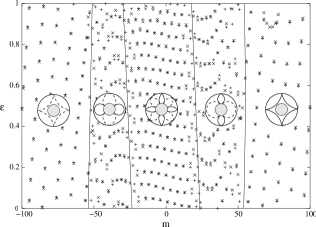
Figure 1: Exact (crosses) and semiclassical (+ signs) energy levels (in units of $\Delta_{0}$) obtained from Eqs. (5a) and (7) as functions of quantum number $m$. In the left/right panel, $k_{\rm F}R_{S}=24.0,18.0$, $\Phi_{\rm miss}=7.2,4.05$, and $R_{S}/R_{N}=0.29981,0.14996$, respectively. For both cases, $\Delta_{0}/E_{\rm F}=0.1$. The solid lines represent the border of regions in the $\varepsilon,m$ plane where the different types of orbits arise. These lines can be obtained from conditions given in Table 1. For easy reference, the different types of orbits are shown in the corresponding regions.

The experimental situation of Ref. Visani, corresponds to the low-magnetic-field limit. There the cyclotron radius is large compared to $R_{N}$, and only orbits of type $A_{2}$ and $B_{2}$ exist in the semiclassical approximation. Therefore, only these two types contribute to the free energy and, ultimately, to the susceptibility. In a simplified model, these orbits have been included in Bruder and Imry’s theoretical study Bruder . Thermodynamical quantities such as the magnetic moment or the susceptibility can be determined from the energy levels of the system Carlo3 . However, to fully explain the experimental results Visani , one needs to extend the work presented in this paper. For example, the Meissner effect can be included in a similar way as in Ref. Uli2, . The energy levels above the bulk superconducting gap ($E>\Delta_{0}$) can be obtained by analytical continuation of the secular equation (5a). One can expect a negligible effect from the roughness of the NS interface if the amplitude of the roughness is less than the wave length of the electrons Klama1-2 ; disord .

In conclusion, we presented a systematic treatment of an experimentally relevant Andreev billiard in a magnetic field using the Bogoliubov-de Gennes formalism. An exact secular equation for Andreev–bound–state levels was derived that we evaluated both numerically and using semiclassical methods. In particular, a classification of possible classical electron and hole orbits in arbitrary magnetic fields was presented. This provides a useful starting point for successive studies of thermodynamic properties because it is possible to obtain the free energy of an NS hybrid system from the quasiparticle energy spectrum. Such an analysis may shed further light on the origin of the recently observed paramagnetic re-entrance effect and opens up a whole arena of new possibilities to study Andreev billiards in magnetic fields.

One of us (J. Cs.) gratefully acknowledges very helpful discussions with C. W. J. Beenakker. This work is supported in part by the European Community’s Human Potential Programme under Contract No. HPRN-CT-2000-00144, Nanoscale Dynamics, the Hungarian-British Intergovernmental Agreement on Cooperation in Education, Culture, Science and Technology, and the Hungarian Science Foundation OTKA TO34832.

References

• (1)
• Hekking et al. (1994) F. W. J. Hekking, G. Schön, and D. V. Averin, eds., Mesoscopic Superconductivity (Elsevier Science, Amsterdam, 1994), special issue of Physica B 203.
• Lambert and Raimondi (1998) C. J. Lambert and R. Raimondi, J. Phys.: Condens. Matter 10, 901 (1998).
• (4) P. Visani, A. C. Mota, and A. Pollini, Phys. Rev. Lett. 65, 1514 (1990); A. C. Mota, P. Visani, A. Pollini, and K. Aupke, Physica B 197, 95 (1994); F. B. Müller-Allinger and A. C. Mota, Phys. Rev. Lett. 84, 3161 (2000).
• (5) C. Bruder and Y. Imry, Phys. Rev. Lett. 80, 5782 (1998).
• (6) A. Fauchère, V. Geshkenbein, and G. Blatter, Phys. Rev. Lett. 82, 1796 (1999); C. Bruder and Y. Imry, ibid. 82, 1797 (1999); A. L. Fauchère, W. Belzig, and G. Blatter, ibid. 82, 3336 (1999); M. Lisowski and E. Zipper, ibid. 86, 1602 (2001); F. Niederer, A. L. Fauchère, and G. Blatter, Phys. Rev. B 65, 132515 (2002).
• (7) S. Pilgram, W. Belzig, and C. Bruder, Phys. Rev. B 62, 12462 (2000).
• (8) A. V. Galaktionov and A. D. Zaikin, cond–mat/0211251 (unpublished).
• (9) P. G. de Gennes, Superconductivity of Metals and Alloys (Benjamin, New York, 1996).
• (10) J. Cserti, A. Bodor, J. Koltai, G. Vattay, Phys. Rev. B 66, 064528 (2002).
• (11) H. Hoppe, U. Zülicke, and G. Schön, Phys. Rev. Lett. 84, 1804 (2000).
• (12) H. Takayanagi and T. Akazaki, Physica B 249-251, 462 (1998); T. D. Moore and D. A. Williams, Phys. Rev. B 59, 7308 (1999); D. Uhlisch et al., ibid. 61, 12463 (2000).
• (13) Y. Takagaki, Phys. Rev. B 57, 4009 (1998); Y. Ishikawa and H. Fukuyama, J. Phys. Soc. Jpn. 68, 954 (1999); Y. Asano, Phys. Rev. B 61, 1732 (2000); N. M. Chtchelkatchev, JETP Lett. 73, 9497 (2001).
• (14) L. Solimany and B. Kramer, Solid State Comm. 96, 471 (1995).
• (15) G. E. Blonder, M. Tinkham, and T. M. Klapwijk, Phys. Rev. B 25, 4515 (1982). Regarding the self-consistency see e.g. references in box_disk:cikk .
• (16) A. Abramowitz and I. A. Stegun, Handbook of Mathematical Functions (Dover Publication, New York, 1972).
• (17) The Andreev approximation amounts to $\Delta_{0}/E_{\rm F}\ll 1$ and quasi particles being incident on/reflected from the interface almost perpendicularly. See, e.g., Ref. Lambert and Raimondi, 1998.
• (18) K. Hornberger and U. Smilansky, Physics Reports 367, 249 (2002); K. Hornberger, Spectral Properties of Magnetic Edge States, Thesis, 2001, München, Germany.
• (19) S. Klama, J. Phys.: Condens. Matter 5, 5609 (1993).
• (20) C. S. Lent, Phys. Rev. B 43, 4179 (1991).
• (21) C. W. J. Beenakker, in Transport Phenomena in Mesoscopic Systems, edited by H. Fukuyama and T. Ando (Springer-Verlag, Berlin, 1992).
• (22) U. Zülicke, H. Hoppe and G. Schön, Physica B 298, 453 (2001).
• (23) L. A. Falkovsky and S. Klama, J. Phys.: Condens. Matter 5, 4491 (1993).