Computing the ground state solution of Bose-Einstein condensates
by a normalized gradient flow

Abstract

In this paper, we prove the energy diminishing of a normalized gradient flow which provides a mathematical justification of the imaginary time method used in physical literatures to compute the ground state solution of Bose-Einstein condensates (BEC). We also investigate the energy diminishing property for the discretization of the normalized gradient flow. Two numerical methods are proposed for such discretizations: one is the backward Euler centered finite difference (BEFD), the other one is an explicit time-splitting sine-spectral (TSSP) method. Energy diminishing for BEFD and TSSP for linear case, and monotonicity for BEFD for both linear and nonlinear cases are proven. Comparison between the two methods and existing methods, e.g. Crank-Nicolson finite difference (CNFD) or forward Euler finite difference (FEFD), shows that BEFD and TSSP are much better in terms of preserving energy diminishing property of the normalized gradient flow. Numerical results in 1d, 2d and 3d with magnetic trap confinement potential, as well as a potential of a stirrer corresponding to a far-blue detuned Gaussian laser beam are reported to demonstrate the effectiveness of BEFD and TSSP methods. Furthermore we observe that the normalized gradient flow can also be applied directly to compute the first excited state solution in BEC when the initial data is chosen as an odd function.

1 Introduction

Since the first experimental realization of Bose-Einstein condensates (BEC) in dilute weakly interacting gases the nonlinear Schrödinger equation (NLS), also called Gross-Pitaevskii equation (GPE) [30, 35], has been used extensively to describe the single particle properties of BECs. The results obtained by solving the NLS showed excellent agreement with most of the experiments (for a review see [5, 17, 16]). In fact, up to now there have been very few experiments in ultracold dilute bosonic gases which could not be described properly by using theoretical methods based on the NLS [25, 28].

There has been a series of recent studies which deal with the numerical solution of the time-independent GPE for ground state and the time-dependent GPE for finding the dynamics of a BEC. For numerical solutions of time-dependent GPE, Bao et al. [6, 7, 9, 10] presented a time-splitting spectral method, Ruprecht et al. [37] used the Crank-Nicolson finite difference method to compute the ground state solution and dynamics of GPE, Cerimele et. al. [14] proposed a particle-inspired scheme. For ground state solution of GPE, Edwards et al. presented a Runge-Kutta type method and used it to solve 1d and 3d with spherical symmetry time-independent GPE [21]. Adhikari [1, 2] used this approach to get the ground state solution of GPE in 2d with radial symmetry. Bao et al. [8] proposed a method by directly minimizing the energy functional. Other approaches include an explicit imaginary-time algorithm used by Chiofalo et al. [15], a direct inversion in the iterated subspace (DIIS) used by Schneider et al. [38], and a simple analytical type method proposed by Dodd [19]. In fact, one of the fundamental problems in numerical simulation of BEC is to compute the ground state solution.

We consider the NLS equation [9, 40]

$$i\;\psi_{t}=-\frac{1}{2}\;\Delta\psi+V({\bf x})\;\psi+\beta|\psi|^{2}\psi,\qquad t>0,\qquad{\bf x}\in\Omega\subseteq{\mathbb{R}}^{d},$$ (1.1)

$$\psi({\bf x},t)=0,\qquad{\bf x}\in\Gamma=\partial\Omega,\quad t\geq 0;$$ (1.2)

where $\Omega$ is a subset of ${\mathbb{R}}^{d}$ and $V({\bf x})$ is a real-valued potential whose shape is determined by the type of system under investigation, and $\beta$ positive/negative corresponds to the defocusing/focusing NLS. (1.1) is known in BEC as the Gross-Pitaevskii equation (GPE) [35] where $\psi$ is the macroscopic wave function of the condensate, $t$ is time, ${\bf x}$ is the spatial coordinate and $V({\bf x})$ is a trapping potential which usually is harmonic and can thus be written as $V({\bf x})=\frac{1}{2}\left(\gamma_{1}^{2}x_{1}^{2}+\cdots+\gamma_{d}^{2}x_{d}^{2}\right)$ with $\gamma_{1},\cdots,\gamma_{d}>0$. Two important invariants of (1.1) are the normalization of the wave function

$$N(\psi)=\int_{\Omega}\;|\psi({\bf x},t)|^{2}\;d{\bf x}=1,\qquad t\geq 0$$ (1.3)

and the energy

$${E_{\beta}}(\psi)=\int_{\Omega}\;\left[\frac{1}{2}|\nabla\psi({\bf x},t)|^{2}+V({\bf x})|\psi({\bf x},t)|^{2}+\frac{\beta}{2}|\psi({\bf x},t)|^{4}\right]\;d{\bf x},\quad t\geq 0.$$ (1.4)

To find a stationary solution of (1.1), we write

$$\psi({\bf x},t)=e^{-i\mu t}\phi({\bf x}),$$ (1.5)

where $\mu$ is the chemical potential of the condensate and $\phi$ a real function independent of time. Inserting into (1.1) gives the following equation for $\phi({\bf x})$

$$\mu\;\phi({\bf x})=-\frac{1}{2}\Delta\phi({\bf x})+V({\bf x})\;\phi({\bf x})+\beta|\phi({\bf x})|^{2}\phi({\bf x}),\qquad{\bf x}\in\Omega,$$ (1.6)

$$\phi({\bf x})=0,\qquad{\bf x}\in\Gamma;$$ (1.7)

under the normalization condition

$$\int_{\Omega}\;|\phi({\bf x})|^{2}\;d{\bf x}=1.$$ (1.8)

This is a nonlinear eigenvalue problem under a constraint and any eigenvalue $\mu$ can be computed from its corresponding eigenfunction $\phi$ by

$$\mu=\mu_{\beta}(\phi) = \int_{\Omega}\left[\frac{1}{2}\left|\nabla\phi({\bf x})\right|^{2}+V({\bf x})\left|\phi({\bf x})\right|^{2}+\beta\left|\phi({\bf x})\right|^{4}\right]d{\bf x}$$ (1.9)

$$= E_{\beta}(\phi)+\int_{\Omega}\;\frac{\beta}{2}\left|\phi({\bf x})\right|^{4}\;d{\bf x}.$$

The non-rotating Bose-Einstein condensate ground state solution $\phi_{g}({\bf x})$ is a real nonnegative function found by minimizing the energy ${E_{\beta}}(\phi)$ under the constraint (1.8) [32]. In physical literatures [3, 13, 15], this minimizer was obtained by applying an imaginary time (i.e. $t\to-it$) in (1.1) and evolving a normalized gradient flow (see details in the next section). In fact, it is easy to show that the minimizer of ${E_{\beta}}(\phi)$ under the constraint (1.8) is an eigenfunction of (1.6).

The aim of this paper is to prove energy diminishing of the normalized gradient flow and present two new numerical methods to discretize the normalized gradient flow. This gives a mathematical justification of the imaginary time method which is widely used in physical literatures to compute the ground state solution of BEC. Energy diminishing of the discretization of the normalized gradient flow is also proven. Extensive numerical results are reported to demonstrate the effectiveness of our new methods.

The paper is organized as follows. In section 2 we prove energy diminishing of the normalized gradient flow and its discretized version. In section 3 we propose two numerical discretizations for the normalized gradient flow. In section 4 numerical comparison between the two methods and existing methods, as well as applications of the two methods for 1d, 2d and 3d ground state solution of BEC, are reported. Finally in section 5 some conclusions are drawn. Throughout we adopt the standard notation for Sobolev spaces.

Before we end the introduction, let us note that the NLS is also used in nonlinear optics, e.g., to describe the propagation of an intense laser beam through a medium with a Kerr nonlinearity [22, 40] where $\psi=\psi({\bf x},t)$ describes the electrical field amplitude, $t$ is the spatial coordinate in the direction of propagation, ${\bf x}=(x_{1},\cdots,x_{d})^{T}$ is the transverse spatial coordinate and $V({\bf x})$ is determined by the index of refraction.

2 Normalized gradient flow

In this section we prove energy diminishing of a normalized gradient flow and its discretized version.

2.1 Energy diminishing

Consider the gradient flow

$$u_{t}=\frac{1}{2}\Delta u-V({\bf x})u-\beta\;|u|^{2}u,\qquad t>0,\quad{\bf x}\in\Omega,$$ (2.1)

$$u({\bf x},0)=u_{0}({\bf x}),\qquad{\bf x}\in\Omega,$$ (2.2)

$$u({\bf x},t)=0,\qquad{\bf x}\in\Gamma,\quad t\geq 0;$$ (2.3)

where $\|u_{0}\|=1$. Here we adopt the norm by $\|\cdot\|=\|\cdot\|_{L^{2}(\Omega)}$ and denote $\|\cdot\|_{L^{m}}=\|\cdot\|_{L^{m}(\Omega)}$ with $m$ an integer. Let

$${\tilde{u}}(\cdot,t)=\frac{u(\cdot,t)}{\|u(\cdot,t)\|},\qquad t\geq 0.$$ (2.4)

Then, it is easy to establish the following basic facts:

Theorem 1.

Suppose $V({\bf x})\geq 0$ for all ${\bf x}\in\Omega$, $\beta\geq 0$ and $\|u_{0}\|=1$, then

(i). $\|u(\cdot,t)\|\leq\|u(\cdot,0)\|=\|u_{0}\|=1$ for $0\leq t<\infty$.

(ii). For any $\beta\geq 0$,

$${E_{\beta}}(u(\cdot,t))\leq{E_{\beta}}(u(\cdot,t^{\prime})),\qquad 0\leq t^{\prime}<t<\infty.$$ (2.5)

(iii). For $\beta=0$,

$${E_{0}}({\tilde{u}}(\cdot,t))\leq{E_{0}}({\tilde{u}}(\cdot,0))={E_{0}}(u_{0}),\qquad 0\leq t<\infty.$$ (2.6)

Proof:  (i). From (2.1) and (2.3), integration by parts, we get

$$\frac{d}{dt}\|u\|^{2} = \frac{d}{dt}\int_{\Omega}u^{2}\;d{\bf x}=\int_{\Omega}2u\;u_{t}\;d{\bf x}=\int_{\Omega}2u\left[\frac{1}{2}\Delta u-V({\bf x})u-\beta|u|^{2}u\right]\;d{\bf x}$$ (2.7)

$$= -2\int_{\Omega}\left[\frac{1}{2}|\nabla u|^{2}+V({\bf x})u^{2}+\beta u^{4}\right]\;d{\bf x}\leq 0,\qquad 0\leq t<\infty.$$

This implies the result in (i).

(ii). From (2.1), (2.3) and (1.4) with $\psi=u$, integration by parts, we get

$$\frac{d}{dt}{E_{\beta}}(u) = 2\int_{\Omega}\left[\frac{1}{2}\nabla u\nabla u_{t}+u_{t}(V({\bf x})u+\beta|u|^{2}u)\right]\;d{\bf x}$$ (2.8)

$$= -2\int_{\Omega}u_{t}\left[\frac{1}{2}\Delta u-V({\bf x})u-\beta|u|^{2}u\right]\;d{\bf x}$$

$$= -2\int_{\Omega}|u_{t}|^{2}\;d{\bf x}\leq 0,\qquad 0\leq t<\infty.$$

This implies the result in (ii).

(iii). From (1.4) with $\psi={\tilde{u}}$ and $\beta=0$, (2.1), (2.3), (2.4), (2.7) and (2.8), integration by parts and Schwartz inequality, we obtain

$$\frac{d}{dt}{E_{0}}({\tilde{u}})=\frac{d}{dt}\int_{\Omega}\left[\frac{|\nabla u|^{2}}{2\|u\|^{2}}+\frac{V({\bf x})u^{2}}{\|u\|^{2}}\right]\;d{\bf x}$$ (2.9)

$$= 2\int_{\Omega}\left[\frac{\nabla u\cdot\nabla u_{t}}{2\|u\|^{2}}+\frac{V({\bf x})u\;u_{t}}{\|u\|^{2}}\right]d{\bf x}-\left(\frac{d}{dt}\|u\|^{2}\right)\;\int_{\Omega}\left[\frac{|\nabla u|^{2}}{2\|u\|^{4}}+\frac{V({\bf x})u^{2}}{\|u\|^{4}}\right]d{\bf x}$$

$$= 2\int_{\Omega}\frac{\left[-\frac{1}{2}\Delta u+V({\bf x})u\right]u_{t}}{\|u\|^{2}}\;d{\bf x}-\left(\frac{d}{dt}\|u\|^{2}\right)\int_{\Omega}\frac{\frac{1}{2}|\nabla u|^{2}+V({\bf x})u^{2}}{\|u\|^{4}}\;d{\bf x}$$

$$= -2\frac{\|u_{t}\|^{2}}{\|u\|^{2}}+\frac{1}{2\|u\|^{4}}\left(\frac{d}{dt}\|u\|^{2}\right)^{2}$$

$$= \frac{2}{\|u\|^{4}}\left[\left(\int_{\Omega}u\;u_{t}\;d{\bf x}\right)^{2}-\|u\|^{2}\|u_{t}\|^{2}\right]$$

$$\leq 0\;,\qquad 0\leq t<\infty.$$

This implies (2.6). $\Box$

Remark 2.1.

The property (2.5) is often referred as the energy diminishing property of the gradient flow. It is interesting to note that (2.6) implies that the energy diminishing property is preserved even in the normalized gradient flow when $\beta=0$, that is, for linear evolution equations.

Remark 2.2.

When $\beta>0$, the solution of (2.1)-(2.2) may not preserve the normalized energy diminishing property

$${E_{\beta}}({\tilde{u}}(\cdot,t))\leq{E_{\beta}}({\tilde{u}}(\cdot,t^{\prime})),\qquad 0\leq t^{\prime}<t<\infty.$$

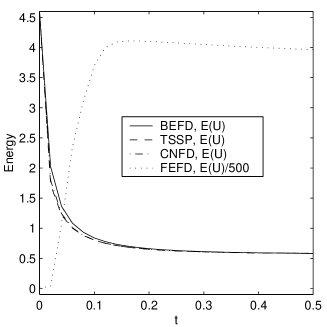
c).   d)

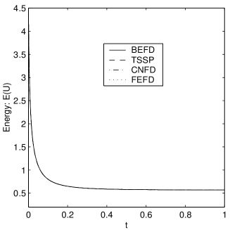
e).   f)

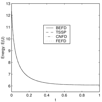
Fig. 1: Energy evolution in Example 1. Left column for case I: a). $k=0.2$, c). $k=0.02$ and e). $k=0.0005$. Right column for case II: b). $k=0.05$, d). $k=0.01$ and f). $k=0.0005$.

In fact, we solve (2.1)-(2.2) in 1d with $\Omega={\mathbb{R}}$ and $V(x)=x^{2}/2$ numerically by the time-splitting spectral method ( see details in the next section) for the initial condition $u_{0}(x)=\displaystyle(\pi/2)^{-1/4}\;e^{-x^{2}}$. Figure 1 shows, for different $\beta$, the energy ${E_{\beta}}({\tilde{u}}(\cdot,t))={E_{\beta}}\left(u(\cdot,t)/\|u(\cdot,t)\|\right)$ under mesh size $h=1/32$ and time step $k=0.0001$. From the figure, we can see that ${E_{\beta}}({\tilde{u}})$ diminishing for $0\leq t<\infty$ when $\beta=0$. But when $\beta>0$, we have ${E_{\beta}}({\tilde{u}})$ diminishing only for $0\leq t\leq t_{0}$ with some finite $t_{0}<\infty$.

Fig. 1: ${E_{\beta}}({\tilde{u}})$ as a function of time in Remark 2.2 for different $\beta$ (labeled as $\delta$).

2.2 Normalized gradient flow

Consider the following continuous normalized gradient flow

$$\phi_{t}=\frac{1}{2}\Delta\phi-V({\bf x})\phi-\beta\;|\phi|^{2}\phi+\mu_{\phi}(t)\phi,\qquad{\bf x}\in\Omega,\quad t\geq 0,$$ (2.10)

$$\phi({\bf x},t)=0,\qquad{\bf x}\in\Gamma,$$ (2.11)

$$\phi({\bf x},0)=\phi_{0}({\bf x}),\qquad{\bf x}\in\Omega.$$ (2.12)

In fact, the right hand side of (2.10) is the same as (1.6) if we view $\mu_{\phi}(t)$ as a Lagrange multiplier for the constraint (1.8). It readily follows that

$$\mu_{\phi}(t)=\frac{1}{\|\phi(\cdot,t)\|^{2}}\int_{\Omega}\left[\frac{1}{2}|\nabla\phi({\bf x},t)|^{2}+V({\bf x})|\phi|^{2}({\bf x},t)+\beta|\phi|^{4}({\bf x},t)\right]d{\bf x}\;.$$ (2.13)

Furthermore for the above normalized gradient flow, as observed in [3, 20], the solution of (2.10) also satisfies the following theorem:

Theorem 2.

Suppose $V({\bf x})\geq 0$ for all ${\bf x}\in\Omega$, $\beta\geq 0$ and $\|\phi_{0}\|=1$. Then the normalized gradient flow (2.10)-(2.12) is normalization conservation and energy diminishing, i.e.

$$\|\phi(\cdot,t)\|^{2}=\int_{\Omega}\phi^{2}({\bf x},t)\;d{\bf x}=\|\phi_{0}\|^{2}=1,\qquad t\geq 0,$$ (2.14)

$$\frac{d}{dt}{E_{\beta}}(\phi)=-2\left\|\phi_{t}(\cdot,t)\right\|^{2}\leq 0\;,\qquad t\geq 0,$$ (2.15)

which in turn implies

$${E_{\beta}}(\phi(\cdot,t_{1}))\geq{E_{\beta}}(\phi(\cdot,t_{2})),\qquad 0\leq t_{1}\leq t_{2}<\infty.$$

Proof:  Multiplying both sides of (2.10) by $\phi$, integrating over $\Omega$, integration by parts and notice (2.13), (2.11), we obtain

$$\frac{1}{2}\frac{d}{dt}\int_{\Omega}|\phi({\bf x},t)|^{2}\;d{\bf x}=\int_{\Omega}\phi\;\phi_{t}\;d{\bf x}$$ (2.16)

$$= \int_{\Omega}\left[\frac{1}{2}\Delta\phi-V({\bf x})\phi-\beta\;\phi^{3}+\mu_{\phi}(t)\phi\right]\phi\;d{\bf x}$$

$$= -\int_{\Omega}\left[\frac{1}{2}|\nabla\phi({\bf x},t)|^{2}+V({\bf x})\phi^{2}({\bf x},t)+\beta\phi^{4}({\bf x},t)\right]d{\bf x}+\mu_{\phi}(t)\|\phi(\cdot,t)\|^{2}$$

$$= 0,\qquad t\geq 0.$$

This implies the normalization conservation (2.14).

Next, direct calculation shows

$$\frac{d}{dt}{E_{\beta}}(\phi) = \int_{\Omega}\left[\frac{1}{2}\nabla\phi\cdot\nabla\phi_{t}+V({\bf x})\phi\phi_{t}+\beta\phi^{3}\phi_{t}\right]d{\bf x}$$ (2.17)

$$= 2\int_{\Omega}\left[-\frac{1}{2}\Delta\phi+V({\bf x})\phi+\beta\phi^{3}\right]\phi_{t}\;d{\bf x}$$

$$= 2\int_{\Omega}\left[-\phi_{t}({\bf x},t)+\mu_{\phi}(t)\phi({\bf x},t)\right]\phi_{t}\;d{\bf x}$$

$$= -2\|\phi_{t}(\cdot,t)\|^{2}+\mu_{\phi}(t)\;\frac{d}{dt}\int_{\Omega}|\phi({\bf x},t)|^{2}\;d{\bf x}$$

$$= -2\|\phi_{t}(\cdot,t)\|^{2}\;,\qquad t\geq 0,$$

since $\mu_{\phi}(t)$ is always real and

$$\frac{d}{dt}\int_{\Omega}|\phi({\bf x},t)|^{2}\;d{\bf x}=0$$

due to the normalization conservation. Thus, we easily get

$${E_{\beta}}(\phi(\cdot,t_{1}))\geq{E_{\beta}}(\phi(\cdot,t_{2})),\qquad 0\leq t_{1}\leq t_{2}<\infty$$

for the solution of (2.10). $\Box$

Remark 2.3.

We see from the above theorem that the energy diminishing property is preserved in the continuous dynamic system (2.10).

Using argument similar to that in [33, 39], we may also get as $t\to\infty$, $\phi$ approaches to a steady state solution which is a critical point of the energy. In non-rotating BEC, it has a unique real valued nonnegative ground state solution $\phi_{g}({\bf x})\geq 0$ for all ${\bf x}\in\Omega$ [32]. We choose the initial data $\phi_{0}({\bf x})\geq 0$ for ${\bf x}\in\Omega$, e.g. the ground state solution of linear Schrödinger equation with a harmonic oscillator potential [8, 9]. Under this kind of initial data, the ground state solution $\phi_{g}$ and its corresponding chemical potential $\mu_{g}$ can be obtained from the steady state solution of the normalized gradient flow (2.10)-(2.12), i.e.

$$\phi_{g}({\bf x})=\lim_{t\to\infty}\phi({\bf x},t),\quad{\bf x}\in\Omega,\qquad\mu_{g}=\mu_{\beta}(\phi_{g})={E_{\beta}}(\phi_{g})+\frac{\beta}{2}\int_{\Omega}\phi_{g}^{4}({\bf x})\;d{\bf x}.$$ (2.18)

2.3 Normalized gradient flow via splitting

Various algorithms for computing the steady state solutions of the normalized gradient flows have been studied in the literature. For instance, second order in time discretization scheme that preserves the norm normalization and energy diminishing properties were presented in [3, 20]. Perhaps one of the more popular technique for dealing with the normalization constraint is through the following construction: choose a time sequence $0=t_{0}<t_{1}<t_{2}<\cdots<t_{n}<\cdots$ with $\Delta t_{n}=t_{n+1}-t_{n}>0$ and $k=\max_{n\geq 0}\;\Delta t_{n}$. To adapt an algorithm for the solution of the usual gradient flow to the case of normalized gradient flow, it is natural to consider the following splitting (or projection) scheme which was widely used in physical literatures [20, 15, 13] for computing the ground state solution of BEC:

$$\phi_{t}=\frac{1}{2}\Delta\phi-V({\bf x})\phi-\beta\;|\phi|^{2}\phi,\qquad{\bf x}\in\Omega,\quad t_{n}<t<t_{n+1},\quad n\geq 0,$$ (2.19)

$$\phi({\bf x},t)=0,\qquad{\bf x}\in\Gamma,$$ (2.20)

$$\phi(x,t_{n+1})\stackrel{{\scriptstyle\triangle}}{{=}}\phi({\bf x},t_{n+1}^{+})=\frac{\phi({\bf x},t_{n+1}^{-})}{\|\phi(\cdot,t_{n+1}^{-})\|},\qquad{\bf x}\in\Omega,\quad n\geq 0,$$ (2.21)

$$\phi({\bf x},0)=\phi_{0}({\bf x}),\qquad{\bf x}\in\Omega;$$ (2.22)

where $\phi({\bf x},t_{n}^{\pm})=\lim_{t\to t_{n}^{\pm}}\phi({\bf x},t)$ and $\|\phi_{0}\|=1$. In fact, (2.19) is the same as the original gradient flow (2.1) which can thus be solved via traditional techniques. The normalization of the gradient flow is simply achieved by a normalization at each discrete time step.

From Theorem 1, we get immediately

Theorem 3.

Suppose $V({\bf x})\geq 0$ for all ${\bf x}\in\Omega$ and $\|\phi_{0}\|=1$. For $\beta=0$, the normalized gradient flow is energy diminishing under any time step $k$ and initial data $\phi_{0}$, i.e.

$${E_{0}}(\phi(\cdot,t_{n+1}))\leq{E_{0}}(\phi(\cdot,t_{n}))\leq\cdots\leq{E_{0}}(\phi(\cdot,0))={E_{0}}(\phi_{0}),\;\;n=0,1,2,\cdots.$$ (2.23)

In fact, the normalized step (2.21) is equivalent to solve the following ODE exactly

$$\phi_{t}({\bf x},t)=\mu_{\phi}(t,k)\phi({\bf x},t),\qquad{\bf x}\in\Omega,\quad t_{n}<t<t_{n+1},\quad n\geq 0,$$ (2.24)

$$\phi({\bf x},t_{n}^{+})=\phi({\bf x},t_{n+1}^{-}),\qquad{\bf x}\in\Omega;$$ (2.25)

where

$$\mu_{\phi}(t,k)\equiv\mu_{\phi}(t_{n+1},\Delta t_{n})=-\frac{1}{2\;\Delta t_{n}}\ln\|\phi(\cdot,t_{n+1}^{-})\|^{2},\qquad t_{n}\leq t\leq t_{n+1}.$$ (2.26)

Thus the normalized gradient flow can be viewed as a first-order splitting method for gradient flow with discontinuous coefficients:

$$\phi_{t}=\frac{1}{2}\Delta\phi-V({\bf x})\phi-\beta\;|\phi|^{2}\phi+\mu_{\phi}(t,k)\phi,\qquad{\bf x}\in\Omega,\quad t\geq 0,$$ (2.27)

$$\phi({\bf x},t)=0,\qquad{\bf x}\in\Gamma,$$ (2.29)

$$\phi({\bf x},0)=\phi_{0}({\bf x}),\qquad{\bf x}\in\Omega.$$

Let $k\to 0$, we see that

$$\lim_{k\to 0^{+}}\mu_{\phi}(t,k)=\mu_{\phi}(t)=\frac{1}{\|\phi(\cdot,t)\|^{2}}\int_{\Omega}\left[\frac{1}{2}|\nabla\phi({\bf x},t)|^{2}+V({\bf x})\phi^{2}({\bf x},t)+\beta\phi^{4}({\bf x},t)\right]d{\bf x},$$ (2.30)

which implies that the problem of (2.27)-(2.29) collapses to (2.10) as $k\to 0$.

Remark 2.4.

As we noted earlier, the energy diminishing property in general does not hold uniformly for all $\phi_{0}$ and all step size $k$. Thus, we propose to consider a modified splitting step which simplifies the computation and yet guarantees the monotonicity when it is discretized by BEFD further.

2.4 Semi-implicit time discretization

To further discretize the equation, we here consider the following semi-implicit time discretization scheme:

$$\frac{{\tilde{\phi}}^{n+1}-\phi^{n}}{k}=\frac{1}{2}\Delta{\tilde{\phi}}^{n+1}-V({\bf x}){\tilde{\phi}}^{n+1}-\beta\;|\phi^{n}|^{2}{\tilde{\phi}}^{n+1}\;,\qquad{\bf x}\in\Omega,$$ (2.31)

$${\tilde{\phi}}^{n+1}({\bf x})=0,\qquad{\bf x}\in\Gamma,$$ (2.32)

$$\phi^{n+1}({\bf x})={\tilde{\phi}}^{n+1}({\bf x})/\|{\tilde{\phi}}^{n+1}\|\;,\qquad{\bf x}\in\Omega\;.$$ (2.33)

Notice that since the equation (2.31) becomes linear, the solution at the new time step becomes relatively simple.

By defining

$${\tilde{V}_{n}({\bf x})}=V({\bf x})+\beta|\phi^{n}({\bf x})|^{2}\;,\qquad{\bf x}\in\Omega,$$

we may rewrite (2.31) as

$$\frac{{\tilde{\phi}}^{n+1}-\phi^{n}}{k}=\frac{1}{2}\Delta{\tilde{\phi}}^{n+1}-{\tilde{V}_{n}({\bf x})}{\tilde{\phi}}^{n+1}\;.$$ (2.34)

In other words, in each discrete time interval, we may view (2.31) as a discretization of a linear gradient flow with a modified potential ${\tilde{V}_{n}({\bf x})}$.

We now first present the following lemma:

Lemma 4.

Suppose ${\tilde{V}_{n}({\bf x})}\geq 0$ for all ${\bf x}\in\Omega$ and $\|\phi^{n}\|=1$. Then,

$$\int_{\Omega}|{\tilde{\phi}}^{n+1}|^{2}\;d{\bf x} \leq \int_{\Omega}\phi^{n}\;{\tilde{\phi}}^{n+1}\;d{\bf x},$$ (2.35)

$$\int_{\Omega}|{\tilde{\phi}}^{n+1}|^{4}\;d{\bf x} \leq \int_{\Omega}|\phi^{n}|^{2}\;|{\tilde{\phi}}^{n+1}|^{2}\;d{\bf x}.$$ (2.36)

Proof:  Multiplying both sides of (2.31) by ${\tilde{\phi}}^{n+1}$, integrating over $\Omega$, and applying integration by parts, we obtain

$$\int_{\Omega}\left(|{\tilde{\phi}}^{n+1}|^{2}-\phi^{n}{\tilde{\phi}}^{n+1}\right)d{\bf x}=-k\int_{\Omega}\left[\frac{1}{2}|\nabla{\tilde{\phi}}^{n+1}|^{2}+{\tilde{V}_{n}({\bf x})}|{\tilde{\phi}}^{n+1}|^{2}\right]d{\bf x}\leq 0\;,$$

which leads to (2.35). Similarly,

$$\int_{\Omega}|{\tilde{\phi}}^{n+1}|^{2}|\phi^{n}|^{2}d{\bf x} = \int_{\Omega}|{\tilde{\phi}}^{n+1}|^{2}\left|{\tilde{\phi}}^{n+1}-\frac{k}{2}\Delta{\tilde{\phi}}^{n+1}+k{\tilde{V}_{n}({\bf x})}{\tilde{\phi}}^{n+1}\right|^{2}d{\bf x}$$ (2.37)

$$= \int_{\Omega}|{\tilde{\phi}}^{n+1}|^{2}\left[|{\tilde{\phi}}^{n+1}|^{2}-2\;\frac{k}{2}{\tilde{\phi}}^{n+1}\Delta{\tilde{\phi}}^{n+1}+2k{\tilde{V}_{n}({\bf x})}|{\tilde{\phi}}^{n+1}|^{2}\right]d{\bf x}$$

$$\qquad+\int_{\Omega}|{\tilde{\phi}}^{n+1}|^{2}\left|\frac{k}{2}\Delta{\tilde{\phi}}^{n+1}-k{\tilde{V}_{n}({\bf x})}{\tilde{\phi}}^{n+1}\right|^{2}d{\bf x}$$

$$= \int_{\Omega}|{\tilde{\phi}}^{n+1}|^{2}\left[|{\tilde{\phi}}^{n+1}|^{2}+3k|\nabla{\tilde{\phi}}^{n+1}|^{2}+2k{\tilde{V}_{n}({\bf x})}|{\tilde{\phi}}^{n+1}|^{2}\right]d{\bf x}$$

$$\qquad+\int_{\Omega}|{\tilde{\phi}}^{n+1}|^{2}\left|\frac{k}{2}\Delta{\tilde{\phi}}^{n+1}-k{\tilde{V}_{n}({\bf x})}{\tilde{\phi}}^{n+1}\right|^{2}d{\bf x}$$

$$\geq \int_{\Omega}|{\tilde{\phi}}^{n+1}|^{4}d{\bf x}\;.$$

This implies (2.36). $\Box$

Given a linear self-adjoint operator $A$ in a Hilbert space $H$ with inner product $(\cdot,\cdot)$, and assume that $A$ is positive definite in the sense that for some positive constant $c$, $(u,Au)\geq c(u,u)$ for any $u\in H$. We now present a simple lemma:

Lemma 5.

For any $k>0$, and $(I+kA)u=v$, we have

$$\frac{(u,Au)}{(u,u)}\leq\frac{(v,Av)}{(v,v)}\;.$$ (2.38)

Proof:  Since $A$ is self-adjoint and positive definite, by Hölder inequality, we have for any $p,q\geq 1$ with $p+q=pq$

$$\left(u,Au\right)\leq\left(u,u\right)^{1/p}\left(u,A^{q}u\right)^{1/q}\;,$$

which leads to

$$\left(u,Au\right)\leq\left(u,u\right)^{1/2}\left(u,A^{2}u\right)^{1/2}\;$$

and

$$\left(u,Au\right)\left(u,A^{2}u\right)\leq\left(u,u\right)\left(u,A^{3}u\right)\;.$$

Direct calculation then gives

$$\left(u,Au\right)\;\left((I+kA)u,(I+kA)u\right)$$ (2.39)

$$= \left(u,Au\right)\;\left(u,u\right)+2k\left(u,Au\right)^{2}+k^{2}\left(u,Au\right)\left(u,A^{2}u\right)$$

$$\leq \left(u,Au\right)\;\left(u,u\right)+2k\left(u,u\right)\;\left(u,A^{2}u\right)+k^{2}\left(u,u\right)\;\left(u,A^{3}u\right)$$

$$= \left(u,u\right)\left((I+kA)u,A(I+kA)u\right).$$

$\Box$

Let us defined a modified energy ${\tilde{E}}_{\phi^{n}}$ as

$${\tilde{E}}_{\phi^{n}}(u)=\int_{\Omega}\left[\frac{1}{2}|\nabla u|^{2}+{\tilde{V}_{n}({\bf x})}|u|^{2}\right]\;d{\bf x}=\int_{\Omega}\left[\frac{1}{2}|\nabla u|^{2}+V({\bf x})|u|^{2}+\beta|\phi^{n}|^{2}|u|^{2}\right]\;d{\bf x}\,,$$

we then get from the above lemma that

Lemma 6.

Suppose $V({\bf x})\geq 0$ for all ${\bf x}\in\Omega$, $\beta\geq 0$ and $\|\phi^{n}\|=1$. Then,

$${\tilde{E}}_{\phi^{n}}({\tilde{\phi}}^{n+1})\leq\frac{{\tilde{E}}_{\phi^{n}}({\tilde{\phi}}^{n+1})}{\|{\tilde{\phi}}^{n+1}\|}={\tilde{E}}_{\phi^{n}}\left(\frac{{\tilde{\phi}}^{n+1}}{\|{\tilde{\phi}}^{n+1}\|}\right)={\tilde{E}}_{\phi^{n}}(\phi^{n+1})\leq{\tilde{E}}_{\phi^{n}}(\phi_{n})\;.$$ (2.40)

Using the inequality (2.36), this in turn implies:

Lemma 7.

Suppose $V({\bf x})\geq 0$ for all ${\bf x}\in\Omega$ and $\beta\geq 0$, then,

$${\tilde{E}_{\beta}}({\tilde{\phi}}^{n+1})\leq{\tilde{E}_{\beta}}(\phi^{n}),$$

where

$${\tilde{E}_{\beta}}(u)=\int_{\Omega}\left[\frac{1}{2}|\nabla u|^{2}+V({\bf x})|u|^{2}+\beta|u|^{4}\right]\;d{\bf x}\,.$$

Remark 2.5.

For $\beta=0$, the energy diminishing property is preserved in the normalized gradient flow via splitting (2.19)-(2.22) and semi-implicit time discretization (2.31)-(2.33). For $\beta>0$, we could only justify the energy diminishing on a modified energy in two adjacent steps.

2.5 Discretized normalized gradient flow

Consider a discretization for the normalized gradient glow (2.31)-(2.33) (or a fully discretization of (2.10)-(2.12))

$$\frac{\tilde{U}^{n+1}-U^{n}}{k}=-A\tilde{U}^{n+1},\qquad U^{n+1}=\frac{\tilde{U}^{n+1}}{\|\tilde{U}^{n+1}\|},\qquad n=0,1,2,\cdots;$$ (2.41)

where $U^{n}=(u_{1}^{n},u_{2}^{n},\cdots,u_{M-1}^{n})^{T}$, $k>0$ is time step and $A$ is an $(M-1)\times(M-1)$ symmetric positive definite matrix. We adopt the inner product, norm and energy of vectors $U=(u_{1},u_{2},\cdots,u_{M-1})^{T}$ and $V=(v_{1},v_{2},\cdots,v_{M-1})^{T}$ as

$$(U,V)=U^{T}V=\sum_{j=1}^{M-1}u_{j}\;v_{j},\quad\|U\|^{2}=U^{T}U=(U,U),\quad{E_{0}}(U)=U^{T}AU=(U,AU),$$ (2.42)

respectively. Using the finite dimensional version of the lemmas given in the previous subsection, we have

Theorem 8.

Suppose $\|U^{0}\|=1$ and $A$ is symmetric positive definite. Then the discretized normalized gradient flow (2.41) is energy diminishing, i.e.

$${E_{0}}\left(U^{n+1}\right)\leq{E_{0}}\left(U^{n}\right)\leq\cdots\leq{E_{0}}\left(U^{0}\right),\qquad n=0,1,2,\cdots.$$ (2.43)

Furthermore if $I+kA$ is an $M$-matrix [24], then $(I+kA)^{-1}$ is a nonnegative matrix (i.e. every entry in it is nonnegative). Thus the flow is monotone, i.e. if $U^{0}$ is a non-negative vector, then $U^{n}$ is also a non-negative vector for all $n\geq 0$.

Remark 2.6.

If a discretization for the normalized gradient flow (2.31)-(2.33) reads

$$\frac{\tilde{U}^{n+1}-U^{n}}{k}=-BU^{n},\qquad U^{n+1}=\frac{\tilde{U}^{n+1}}{\|\tilde{U}^{n+1}\|},\qquad n=0,1,2,\cdots.$$ (2.44)

Suppose $B$ is symmetric and positive definite and $\rho(kB)<1$ where $\rho(B)$ refers to the spectral radius of the matrix $B$. Then (2.43) is satisfied by choosing

$$A=\frac{1}{k}\left(\left(I-kB\right)^{-1}-I\right)=\left(I-kB\right)^{-1}B.$$

Remark 2.7.

If a discretization for the normalized gradient flow (2.31)-(2.33) reads

$$\tilde{U}^{n+1}=BU^{n},\qquad U^{n+1}=\frac{\tilde{U}^{n+1}}{\|\tilde{U}^{n+1}\|},\qquad n=0,1,2,\cdots.$$ (2.45)

Suppose $B$ is symmetric and positive definite and $\rho(B)<1$. Then (2.43) is satisfied by choosing

$$A=\frac{1}{k}\left(B^{-1}-I\right).$$

Remark 2.8.

If a discretization for the normalized gradient flow (2.31)-(2.33) reads

$$\frac{\tilde{U}^{n+1}-U^{n}}{k}=-B\tilde{U}^{n+1}-CU^{n},\quad U^{n+1}=\frac{\tilde{U}^{n+1}}{\|\tilde{U}^{n+1}\|},\quad n=0,1,2,\cdots.$$ (2.46)

Suppose $B$ and $C$ are symmetric, positive definite and $\rho(kC)<1$. Then (2.43) is satisfied by choosing

$$A=\left(I-kC\right)^{-1}(B+C).$$

3 Numerical methods and energy diminishing

In this section, we will present two numerical methods to discretize the normalized gradient flow (2.19)-(2.22). For simplicity of notation we shall introduce the methods for the case of one spatial dimension $(d=1)$ with homogeneous periodic boundary conditions. Generalizations to $d>1$ are straightforward for tensor product grids and the results remain valid without modifications. For $d=1$, the problem becomes

$$\phi_{t}=\frac{1}{2}\phi_{xx}-V(x)\phi-\beta\;|\phi|^{2}\phi,\quad x\in\Omega=(a,b),\ t_{n}<t<t_{n+1},\ n\geq 0,\qquad$$ (3.1)

$$\phi(x,t_{n+1})\stackrel{{\scriptstyle\triangle}}{{=}}\phi(x,t_{n+1}^{+})=\frac{\phi(x,t_{n+1}^{-})}{\|\phi(\cdot,t_{n+1}^{-})\|},\qquad a\leq x\leq b,\quad n\geq 0,$$ (3.2)

$$\phi(x,0)=\phi_{0}(x),\qquad a\leq x\leq b,$$ (3.3)

$$\phi(a,t)=\phi(b,t)=0,\qquad t\geq 0;$$ (3.4)

with

$$\|\phi_{0}\|^{2}=\int_{a}^{b}\phi_{0}^{2}(x)\;dx=1.$$

3.1 Numerical methods

We choose the spatial mesh size $h=\Delta x>0$ with $h=(b-a)/M$ and $M$ an even positive integer, the time step is given by $k=\Delta t>0$ and define grid points and time steps by

$$x_{j}:=a+j\;h,\qquad t_{n}:=n\;k,\qquad j=0,1,\cdots,M,\qquad n=0,1,2,\cdots$$

Let $\phi^{n}_{j}$ be the numerical approximation of $\phi(x_{j},t_{n})$ and $\phi^{n}$ the solution vector at time $t=t_{n}=nk$ with components $\phi_{j}^{n}$.

Backward Euler finite difference (BEFD) We use backward Euler for time discretization and second-order centered finite difference for spatial derivatives. The detail scheme is:

$$\frac{\phi_{j}^{*}-\phi_{j}^{n}}{k}=\frac{1}{2h^{2}}\left[\phi_{j+1}^{*}-2\phi_{j}^{*}+\phi_{j-1}^{*}\right]-V(x_{j})\phi_{j}^{*}-\beta\left(\phi_{j}^{n}\right)^{2}\phi_{j}^{*},\quad j=1,\cdots,M-1,$$

$$\phi_{0}^{*}=\phi_{M}^{*}=0,$$

$$\phi_{j}^{n+1}=\frac{\phi_{j}^{*}}{\|\phi^{*}\|},\qquad j=0,\cdots,M,\qquad n=0,1,\cdots,$$ (3.5)

$$\phi_{j}^{0}=\phi_{0}(x_{j}),\qquad j=0,1,\cdots,M;$$

where the norm is defined as

$$\|\phi^{*}\|^{2}=h\sum_{j=1}^{M-1}\left(\phi_{j}^{*}\right)^{2}.$$

Time-splitting sine-spectral method (TSSP) From time $t=t_{n}$ to time $t=t_{n+1}$, the equation (3.1) is solved in two steps. One solves

$$\phi_{t}=\frac{1}{2}\phi_{xx},$$ (3.6)

for one time step of length $k$, followed by solving

$$\phi_{t}(x,t)=-V(x)\phi(x,t)-\beta|\phi|^{2}\phi(x,t),\qquad t_{n}\leq t\leq t_{n+1},$$ (3.7)

again for the same time step. Equation (3.6) is discretized in space by the sine-spectral method and integrated in time exactly. For $t\in[t_{n},t_{n+1}]$, multiplying the ODE (3.7) by $\phi(x,t)$, one obtains with $\rho(x,t)=\phi^{2}(x,t)$

$$\rho_{t}(x,t)=-2V(x)\rho(x,t)-2\beta\rho^{2}(x,t),\qquad t_{n}\leq t\leq t_{n+1}.$$ (3.8)

The solution of the ODE (3.8) can be expressed as

$$\rho(x,t)=\left\{\begin{array}[]{ll}\displaystyle\frac{V(x)\rho(x,t_{n})}{\left(V(x)+\beta\rho(x,t_{n})\right)e^{2V(x)(t-t_{n})}-\beta\rho(x,t_{n})}&\qquad V(x)\neq 0,\\ \\ \displaystyle\frac{\rho(x,t_{n})}{1+2\beta\rho(x,t_{n})(t-t_{n})},&\qquad V(x)=0.\end{array}\right.$$ (3.9)

Combining the splitting step via the standard second-order Strang splitting for solving the normalized gradient flow (3.1)-(3.4), in detail, the steps for obtaining $\phi_{j}^{n+1}$ from $\phi_{j}^{n}$ are given by

$$\phi^{*}_{j}=\left\{\begin{array}[]{ll}\displaystyle\sqrt{\frac{V(x_{j})e^{-kV(x_{j})}}{V(x_{j})+\beta(1-e^{-kV(x_{j})})|\phi_{j}^{n}|^{2}}}\ \phi_{j}^{n}&\qquad V(x_{j})\neq 0,\\ \\ \displaystyle\frac{1}{\sqrt{1+\beta k|\phi_{j}^{n}|^{2}}}\ \phi_{j}^{n},&\qquad V(x_{j})=0,\end{array}\right.$$ (3.13)

$$\phi_{j}^{**}=\sum_{l=1}^{M-1}e^{-k\mu_{l}^{2}/2}\;\widehat{\phi}^{*}_{l}\;\sin(\mu_{l}(x_{j}-a)),\qquad j=1,2,\cdots,M-1,$$

$$\phi^{***}_{j}=\left\{\begin{array}[]{ll}\displaystyle\sqrt{\frac{V(x_{j})e^{-kV(x_{j})}}{V(x_{j})+\beta(1-e^{-kV(x_{j})})|\phi_{j}^{**}|^{2}}}\ \phi_{j}^{**}&\qquad V(x_{j})\neq 0,\\ \\ \displaystyle\frac{1}{\sqrt{1+\beta k|\phi_{j}^{**}|^{2}}}\ \phi_{j}^{**},&\qquad V(x_{j})=0,\end{array}\right.$$ (3.17)

$$\phi_{j}^{n+1}=\frac{\phi_{j}^{***}}{\|\phi^{***}\|},\qquad j=0,\cdots,M,\qquad n=0,1,\cdots;$$ (3.18)

where $\widehat{U}_{l}$ are the sine-transform coefficients of a real vector $U=(u_{0},u_{1},\cdots,u_{M})^{T}$ with $u_{0}=u_{M}=0$ which are defined as

$$\mu_{l}=\frac{\pi l}{b-a},\quad\widehat{U}_{l}=\frac{2}{M}\sum_{j=1}^{M-1}u_{j}\;\sin(\mu_{l}(x_{j}-a)),\quad l=1,2,\cdots,M-1$$ (3.19)

and

$$\phi^{0}_{j}=\phi(x_{j},0)=\phi_{0}(x_{j}),\qquad j=0,1,2,\cdots,M.$$

Note that the only time discretization error of TSSP is the splitting error, which is second order in $k$.

For comparison purposes we review a few other numerical methods which are currently used for solving the normalized gradient flow. One is the Crank-Nicolson finite difference (CNFD) scheme [23]:

$$\frac{\phi_{j}^{*}-\phi_{j}^{n}}{k}=\frac{1}{4h^{2}}\left[\phi_{j+1}^{*}-2\phi_{j}^{*}+\phi_{j-1}^{*}+\phi_{j+1}^{n}-2\phi_{j}^{n}+\phi_{j-1}^{n}\right]$$

$$\qquad\qquad-\frac{V(x_{j})}{2}\left[\phi_{j}^{*}+\phi_{j}^{n}\right]-\frac{\beta\left|\phi_{j}^{n}\right|^{2}}{2}\left[\phi_{j}^{*}+\phi_{j}^{n}\right],\qquad j=1,\cdots,M-1,$$

$$\phi_{0}^{*}=\phi_{M}^{*}=0,$$

$$\phi_{j}^{n+1}=\frac{\phi_{j}^{*}}{\|\phi^{*}\|},\qquad j=0,\cdots,M,\qquad n=0,1,\cdots,$$ (3.20)

$$\phi_{j}^{0}=\phi_{0}(x_{j}),\qquad j=0,1,\cdots,M.$$

Another one is the forward Euler finite difference (FEFD) method [15]:

$$\frac{\phi_{j}^{*}-\phi_{j}^{n}}{k}=\frac{1}{2h^{2}}\left[\phi_{j+1}^{n}-2\phi_{j}^{n}+\phi_{j-1}^{n}\right]-V(x_{j})\phi_{j}^{n}-\beta\left|\phi_{j}^{n}\right|^{2}\phi_{j}^{n},\qquad j=1,\cdots,M-1,$$

$$\phi_{0}^{*}=\phi_{M}^{*}=0,$$

$$\phi_{j}^{n+1}=\frac{\phi_{j}^{*}}{\|\phi^{*}\|},\qquad j=0,\cdots,M,\qquad n=0,1,\cdots,$$ (3.21)

$$\phi_{j}^{0}=\phi_{0}(x_{j}),\qquad j=0,1,\cdots,M;$$

3.2 Energy diminishing

First we analyze the energy diminishing of the different numerical methods for linear case, i.e. $\beta=0$ in (3.1). Introducing

$$\Phi^{n}=\left(\phi_{1}^{n},\;\phi_{2}^{n},\;\cdots,\;\phi_{M-1}^{n}\right)^{T},$$

$$D=\left(d_{jl}\right)_{(M-1)\times(M-1)},\quad\hbox{with}\ d_{jl}=\frac{1}{2h^{2}}\left\{\begin{array}[]{ll}2&j=l,\\ -1&|j-l|=-1,\\ 0&\hbox{otherwise},\end{array}\right.\quad j,l=1,\cdots,M-1,$$

$$E={\rm diag}\left(V(x_{1}),\;V(x_{2}),\;\cdots,\;V(x_{M-1})\right),$$

$$F(\Phi)={\rm diag}\left(\phi_{1}^{2},\;\phi_{2}^{2},\;\cdots,\;\phi_{M-1}^{2}\right),\qquad\hbox{with}\quad\Phi=\left(\phi_{1},\;\phi_{2},\;\cdots,\;\phi_{M-1}\right)^{T},$$

$$G=\left(g_{jl}\right)_{(M-1)\times(M-1)},\qquad\hbox{with}\ g_{jl}=\frac{2}{M}\sum_{m=1}^{M-1}\sin\frac{\pi mj}{M}\;\sin\frac{\pi ml}{M}\;e^{-k\mu_{m}^{2}/2},$$

$$H={\rm diag}\left(e^{-kV(x_{1})/2},\;e^{-kV(x_{2})/2},\;\cdots,\;e^{-kV(x_{M-1})/2}\right).$$

Then the BEFD discretization (3.5) (called BEFD normalized flow) with $\beta=0$ can be expressed as

$$\frac{\Phi^{*}-\Phi^{n}}{k}=-(D+E)\Phi^{*},\quad\Phi^{n+1}=\frac{\Phi^{*}}{\|\Phi^{*}\|},\qquad n=0,1,\cdots.$$ (3.23)

The TSSP discretization (3.17) (called TSSP normalized flow) with $\beta=0$ can be expressed as

$$\Phi^{***}=H\Phi^{**}=HG\Phi^{*}=HGH\Phi^{n},\qquad\Phi^{n+1}=\frac{\Phi^{*}}{\|\Phi^{*}\|},\qquad n=0,1,\cdots.$$ (3.24)

The CNFD discretization (3.20) (called CNFD normalized flow) with $\beta=0$ can be expressed as

$$\frac{\Phi^{*}-\Phi^{n}}{k}=-\frac{1}{2}(D+E)\Phi^{*}-\frac{1}{2}(D+E)\Phi^{n},\quad\Phi^{n+1}=\frac{\Phi^{*}}{\|\Phi^{*}\|},\qquad n=0,1,\cdots.$$ (3.25)

The FEFD discretization (3.21) (called FEFD normalized flow) with $\beta=0$ can be expressed as

$$\frac{\Phi^{*}-\Phi^{n}}{k}=-(D+E)\Phi^{n},\quad\Phi^{n+1}=\frac{\Phi^{*}}{\|\Phi^{*}\|},\qquad n=0,1,\cdots.$$ (3.26)

It is easy to see that $D$ and $G$ are symmetric positive definite matrices. Furthermore $D$ is also an $M$-matrix and $\rho(D)=\left(1+\cos\frac{\pi}{M}\right)/h^{2}<2/h^{2}$ and $\rho(G)=e^{-k\mu_{1}^{2}/2}<1$. Applying Theorem 8 and Remarks 2.6,2.7&2.8, we have

Theorem 9.

Suppose $V(x)\geq 0$ and $\beta=0$. We have that

(i). The BEFD normalized flow (3.5) is energy diminishing and monotone for any $k>0$.

(ii). The TSSP normalized flow (3.17) is energy diminishing for any $k>0$.

(iii). The CNFD normalized flow (3.20) is energy diminishing and monotone provided that

$$k\leq\frac{2}{2/h^{2}+\max_{j}V(x_{j})}=\frac{2h^{2}}{2+h^{2}\;\max_{j}V(x_{j})}.$$ (3.27)

(iv). The FEFD normalized flow (3.21) is energy diminishing and monotone provided that

$$k\leq\frac{1}{2/h^{2}+\max_{j}V(x_{j})}=\frac{h^{2}}{2+h^{2}\;\max_{j}V(x_{j})}.$$ (3.28)

For nonlinear case, i.e. $\beta>0$, we only analyze the energy between two steps of BEFD flow (3.5). In this case, consider

$$\frac{\tilde{\Phi}^{n+1}-\Phi^{n}}{k}=-\left(D+E+\beta F(\Phi^{n})\right)\tilde{\Phi}^{n+1},\qquad\Phi^{n+1}=\frac{\tilde{\Phi}^{n+1}}{\|\tilde{\Phi}^{n+1}\|}.$$ (3.29)

Lemma 10.

Suppose $V(x)\geq 0$, $\beta>0$ and $\|\Phi^{n}\|=1$. Then for the flow (3.29), we have

$${\tilde{E}_{\beta}}\left(\tilde{\Phi}^{n+1}\right)\leq{\tilde{E}_{\beta}}\left(\Phi^{n}\right),\qquad\tilde{E}_{\Phi^{n}}\left(\Phi^{n+1}\right)\leq\tilde{E}_{\Phi^{n}}\left(\Phi^{n}\right)$$ (3.30)

where

$${\tilde{E}_{\beta}}\left(\Phi\right) = (\Phi,(D+E+\beta F(\Phi))\Phi)=\Phi^{T}(D+E)\Phi+\beta\sum_{j=1}^{M-1}\phi_{j}^{4},$$ (3.31)

$$\tilde{E}_{\Phi^{n}}\left(\Phi\right) = (\Phi,(D+E+\beta F(\Phi^{n}))\Phi)=\Phi^{T}(D+E)\Phi+\beta\sum_{j=1}^{M-1}\phi_{j}^{2}\;\left(\phi^{n}_{j}\right)^{2}\;.\qquad$$ (3.32)

Proof:  Combining (3.29), (2.41) and Theorem 8, we have

$$\left(\tilde{\Phi}^{n+1},\;(D+E+\beta F(\Phi^{n}))\tilde{\Phi}^{n+1}\right)\leq\frac{\left(\tilde{\Phi}^{n+1},\;(D+E+\beta F(\Phi^{n}))\tilde{\Phi}^{n+1}\right)}{\left(\tilde{\Phi}^{n+1},\tilde{\Phi}^{n+1}\right)}$$ (3.33)

$$\qquad\leq\frac{\left(\Phi^{n},\;(D+E+\beta F(\Phi^{n}))\Phi^{n}\right)}{\left(\Phi^{n},\Phi^{n}\right)}={\tilde{E}_{\beta}}\left(\Phi^{n}\right).$$

Similar to the proof of (2.36), we have

$$\sum_{j=1}^{M-1}\left(\phi_{j}^{n}\right)^{2}\left(\tilde{\phi}_{j}^{n+1}\right)^{2}\geq\sum_{j=1}^{M-1}\left(\tilde{\phi}_{j}^{n+1}\right)^{4}.$$ (3.34)

The required result (3.30) is a combination of (3.34), and (3.33). $\Box$

4 Numerical results

In this section we compare the four different numerical discretizations for normalized gradient flow and report numerical results of the ground state solutions of BEC in 1d, 2d and 3d with magnetic trap confinement potential. We also compute the ground state solutions with the potential of a stirrer corresponding a far-blue detuned Gaussian laser beam and central vortex state by the methods BEFD or TSSP.

Due to the ground state solution $\phi_{g}({\bf x})\geq 0$ for ${\bf x}\in\Omega$ in non-rotating BEC [32], in our computations, the initial condition (2.22) is always chosen such that $\phi_{0}({\bf x})\geq 0$ and decays to zero sufficiently fast as $|{\bf x}|\to\infty$. We choose an appropriately large interval, rectangle and box in 1d, 2d and 3d, respectively, to avoid that the homogeneous periodic boundary condition (3.4) introduce a significant (aliasing) error relative to the whole space problem. To quantify the ground state solution $\phi_{g}({\bf x})$, we define the radius mean square

$$\alpha_{\rm rms}=\|\alpha\phi_{g}\|_{L^{2}(\Omega)}=\sqrt{\int_{\Omega}\alpha^{2}\phi_{g}^{2}({\bf x})\;d{\bf x}},\qquad\alpha=x,y,\ {\rm or}\ z.$$ (4.1)

4.1 Comparisons of different methods

Example 1 Normalized gradient flow in 1d, i.e. $d=1$ in (2.19)-(2.22). We consider two cases:

I. Linear case ($\beta=0$) with a double-well potential,

$$V(x)=\frac{1}{2}(1-x^{2})^{2},\qquad\beta=0,\quad\phi_{0}(x)=\frac{1}{(4\pi)^{1/4}}e^{-x^{2}/8},\quad x\in{\mathbb{R}}.$$

II. Nonlinear case ($\beta>0$) with a harmonic oscillator potential,

$$V(x)=\frac{x^{2}}{2},\qquad\beta=60,\quad\phi_{0}(x)=\frac{1}{(\pi)^{1/4}}e^{-x^{2}/2},\quad x\in{\mathbb{R}}.$$

The case I is solved on $\Omega=[-16,16]$ and the case II on $\Omega=[-8,8]$ with mesh size $h=\frac{1}{32}$. Figure 4.1 shows the evolution of the energy ${E_{\beta}}(\phi)$ for different time step $k$ and different numerical methods.

From Figure 4.1, the following observations can be made:

(1). BEFD is an implicit method and energy diminishing is observed for both linear and the nonlinear case under any time step $k>0$. The error in the ground state solution is only due to the second order spatial discretization.

(2). TSSP is an explicit method and energy diminishing is observed for linear case under any time step $k>0$. For nonlinear case, our numerical experiments show that $k<\frac{1}{\beta}$ guarantees energy diminishing. The error in the ground state solution is caused by both the spatial discretization which is spectral accuracy and time splitting which is second-order accuracy. From accuracy point of view, large values of $k$ should be prohibited.

(3). CNFD is an implicit method and FEFD is an explicit method. For both schemes, energy diminishing is observed only when the time step $k$ satisfies the condition (3.27) and (3.28), respectively.

To summarize briefly, in general, BEFD is much better than CNFD for computing the ground state solution because BEFD is monotone for any $k>0$ and CNFD is not. TSSP is much better than FEFD. In practice, one can use either BEFD or TSSP. BEFD allows the use of much bigger time step $k$ which does not depend on $\beta\geq 0$, but the scheme has only second order accuracy in space. At each time step, a linear system is solved. In the appendix, we give the detailed BEFD discretization in 2d and 3d when the potential $V({\bf x})$ and the initial data $\phi_{0}({\bf x})$ have symmetry with/without a central vortex state in the condensate. TSSP is explicit, easy to program, less demanding on memory and spectrally accurate in space, but it needs a small time step $k$ which depends on the accuracy required and the value of $\beta>0$, but not on the mesh size $h$. Based on our numerical experiments given in the next subsection, both methods work very well for computing the ground state solution of BEC.

4.2 Applications to ground state solutions

Example 2 Ground state solution of BEC in 1d with harmonic oscillator potential, i.e.

$$V(x)=\frac{x^{2}}{2},\qquad\phi_{0}(x)=\frac{1}{(\pi)^{1/4}}e^{-x^{2}/2},\quad x\in{\mathbb{R}}.$$

The normalized gradient flow (2.19)-(2.22) with $d=1$ is solved on $\Omega=[-16,16]$ with mesh size $h=\frac{1}{8}$ and time step $k=0.001$ by using TSSP. The steady state solution is reached when $\max\left|\Phi^{n+1}-\Phi^{n}\right|<\varepsilon=10^{-6}$. Figure 4.2 shows the ground state solution $\phi_{g}(x)$ and energy evolution for different $\beta$. Table 1 displays the values of $\phi_{g}(0)$, radius mean square $x_{\rm rms}$, energy ${E_{\beta}}(\phi_{g})$ and chemical potential $\mu_{g}$.

Table 1: Maximum value of the wave function $\phi_{g}(0)$, root mean square size $x_{\rm rms}$, energy ${E_{\beta}}(\phi_{g})$ and ground state chemical potential $\mu_{g}$ versus the interaction coefficient $\beta$ in 1d.

$\beta$	$\phi_{g}(0)$	$x_{\rm rms}$	${E_{\beta}}(\phi_{g})$	$\mu_{g}=\mu_{\beta}(\phi_{g})$
0	0.7511	0.7071	0.5000	0.5000
3.1371	0.6463	0.8949	1.0441	1.5272
12.5484	0.5301	1.2435	2.2330	3.5986
31.371	0.4562	1.6378	3.9810	6.5587
62.742	0.4067	2.0423	6.2570	10.384
156.855	0.3487	2.7630	11.464	19.083
313.71	0.3107	3.4764	18.171	30.279
627.42	0.2768	4.3757	28.825	48.063
1254.8	0.2467	5.5073	45.743	76.312

The results in Figure 4.2 and Table 1 agree very well with the ground state solutions of BEC obtained by a direct minimization the energy functional [8]. BEFD gives the same results with $k=0.1$.

Example 3 Ground state solution of BEC in 2d. Two cases are considered:

I. With a harmonic oscillator potential [8, 9, 21], i.e.

$$V(x,y)=\frac{1}{2}\left(\gamma_{x}^{2}x^{2}+\gamma_{y}^{2}y^{2}\right).$$

II. With a harmonic oscillator potential and a potential of a stirrer corresponding a far-blue detuned Gaussian laser beam [27] which is used to generate vortices in BEC [11], i.e.

$$V(x,y)=\frac{1}{2}\left(\gamma_{x}^{2}x^{2}+\gamma_{y}^{2}y^{2}\right)+w_{0}e^{-\delta((x-r_{0})^{2}+y^{2})}.$$

The initial condition is chosen as

$$\phi_{0}(x,y)=\frac{(\gamma_{x}\gamma_{y})^{1/4}}{\pi^{1/2}}e^{-(\gamma_{x}x^{2}+\gamma_{y}y^{2})/2}.$$

For case I, we choose $\gamma_{x}=1$, $\gamma_{y}=4$, $w_{0}=\delta=r_{0}=0$, $\beta=200$ and solve the problem by TSSP on $\Omega=[-8,8]\times[-4,4]$ with mesh size $h_{x}=\frac{1}{8}$, $h_{y}=\frac{1}{16}$ and time step $k=0.001$. We get the following results from the ground state solution $\phi_{g}$:

$$x_{\rm rms}=2.2734,\ y_{\rm rms}=0.6074,\ \phi_{g}^{2}(0)=0.0808,\ {E_{\beta}}(\phi_{g})=11.1563,\ \mu_{g}=16.3377.$$

For case II, we choose $\gamma_{x}=1$, $\gamma_{y}=1$, $w_{0}=4$, $\delta=r_{0}=1$, $\beta=200$ and solve the problem by TSSP on $\Omega=[-8,8]^{2}$ with mesh size $h=\frac{1}{8}$ and time step $k=0.001$. We get the following results from the ground state solution $\phi_{g}$:

$$x_{\rm rms}=1.6951,\ y_{\rm rms}=1.7144,\ \phi_{g}^{2}(0)=0.034,\ {E_{\beta}}(\phi_{g})=5.8507,\ \mu_{g}=8.3269.$$

In addition, Figure 4.3 shows surface plots of the ground state solution $\phi_{g}$. BEFD gives similar results with $k=0.1$.

Example 4 Ground state solution of BEC in 3d. Two cases are considered:

I. With a harmonic oscillator potential [8, 9, 21], i.e.

$$V(x,y,z)=\frac{1}{2}\left(\gamma_{x}^{2}x^{2}+\gamma_{y}^{2}y^{2}+\gamma_{z}^{2}z^{2}\right).$$

II. With a harmonic oscillator potential and a potential of a stirrer corresponding a far-blue detuned Gaussian laser beam [27, 12] which is used to generate vortex in BEC [12], i.e.

$$V(x,y,z)=\frac{1}{2}\left(\gamma_{x}^{2}x^{2}+\gamma_{y}^{2}y^{2}+\gamma_{z}^{2}z^{2}\right)+w_{0}e^{-\delta((x-r_{0})^{2}+y^{2})}.$$

The initial condition is chosen as

$$\phi_{0}(x,y,z)=\frac{(\gamma_{x}\gamma_{y}\gamma_{z})^{1/4}}{\pi^{3/4}}e^{-(\gamma_{x}x^{2}+\gamma_{y}y^{2}+\gamma_{z}z^{2})/2}.$$

For case I, we choose $\gamma_{x}=1$, $\gamma_{y}=2$, $\gamma_{z}=4$, $w_{0}=\delta=r_{0}=0$, $\beta=200$ and solve the problem by TSSP on $\Omega=[-8,8]\times[-6,6]\times[-4,4]$ with mesh size $h_{x}=\frac{1}{8}$, $h_{y}=\frac{3}{32}$, $h_{z}=\frac{1}{16}$ and time step $k=0.001$. The ground state solution $\phi_{g}$ gives:

$$x_{\rm rms}=1.67,\ y_{\rm rms}=0.87,\ z_{\rm rms}=0.49,\ \phi_{g}^{2}(0)=0.052,\ {E_{\beta}}(\phi_{g})=8.33,\ \mu_{g}=11.03.$$

For case II, we choose $\gamma_{x}=1$, $\gamma_{y}=1$, $\gamma_{z}=2$, $w_{0}=4$, $\delta=r_{0}=1$, $\beta=200$ and solve the problem by TSSP on $\Omega=[-8,8]^{3}$ with mesh size $h=\frac{1}{8}$ and time step $k=0.001$. The ground state solution $\phi_{g}$ gives:

$$x_{\rm rms}=1.37,\ y_{\rm rms}=1.43,\ z_{\rm rms}=0.70,\ \phi_{g}^{2}(0)=0.025,\ {E_{\beta}}(\phi_{g})=5.27,\ \mu_{g}=6.71.$$

Furthermore, Figure 4.4 shows surface plots of the ground state solution $\phi_{g}^{2}(x,0,z)$. BEFD gives similar results with $k=0.1$.

Example 5 2d central vortex states in BEC, i.e.

$$V(x,y)=V(r)=\frac{1}{2}\left(\frac{m^{2}}{r^{2}}+r^{2}\right),\ \phi_{0}(x,y)=\phi_{0}(r)=\frac{1}{\sqrt{\pi m!}}\;r^{m}\;e^{-r^{2}/2},\ 0\leq r.$$

The normalized gradient flow is solved in polar coordinate with $\Omega=[0,8]$ with mesh size $h=\frac{1}{64}$ and time step $k=0.1$ by using BEFD (see detail in Appendix A3). Figure 4.5a shows the ground state solution $\phi_{g}(r)$ with $\beta=200$ for different index of the central vortex $m$. Table 2 displays the values of $\phi_{g}(0)$, radius mean square $r_{\rm rms}$, energy ${E_{\beta}}(\phi_{g})$ and chemical potential $\mu_{g}$.

Table 2: Numerical results for 2d central vortex states in BEC.

Index $m$	$\phi_{g}(0)$	$r_{\rm rms}$	${E_{\beta}}(\phi_{g})$	$\mu_{g}=\mu_{\beta}(\phi_{g})$
1	0.0000	2.4086	5.8014	8.2967
2	0.0000	2.5258	6.3797	8.7413
3	0.0000	2.6605	7.0782	9.3160
4	0.0000	2.8015	7.8485	9.9772
5	0.0000	2.9438	8.6660	10.6994
6	0.0000	3.0848	9.5164	11.4664

4.3 Application to compute the first excited state

Suppose the eigenfunctions of the nonlinear eigenvalue problem (1.6), (1.7) under the constraint (1.8) are

$$\pm\phi_{g}({\bf x}),\ \pm\phi_{1}({\bf x}),\ \pm\phi_{2}({\bf x}),\ \cdots,$$

whose energies satisfy

$${E_{\beta}}(\phi_{g})<{E_{\beta}}(\phi_{1})<{E_{\beta}}(\phi_{2})<\cdots\;.$$

Then $\phi_{j}$ is called as the $j$-th excited state solution. In fact, $\phi_{g}$ and $\phi_{j}$ ($j=1,2,\cdots$) are critical points of the energy functional $E_{\beta}(\phi)$ under the constraint (1.8). In 1d, when $V(x)=\frac{x^{2}}{2}$ is chosen as the harmonic oscillator potential, the first excited state solution $\phi_{1}(x)$ is a real odd function, and $\phi_{1}(x)=\frac{\sqrt{2}}{(\pi)^{1/4}}\;x\;e^{-x^{2}/2}$ when $\beta=0$ [31]. We observe numerically that the normalized gradient flow (2.19)-(2.22) and its BEFD discretization (3.5) can also be applied directly to compute the first excited state solution, i.e. $\phi_{1}(x)$, provided that the initial data $\phi_{0}(x)$ in (2.22) is chosen as an odd function. Here we only present a preliminary numerical example in 1d. Extensions to 2d and 3d are straightforward.

Example 6 First excited state solution of BEC in 1d with a harmonic oscillator potential, i.e.

$$V(x)=\frac{x^{2}}{2},\qquad\phi_{0}(x)=\frac{\sqrt{2}}{(\pi)^{1/4}}\;x\;e^{-x^{2}/2},\quad x\in{\mathbb{R}}.$$

The normalized gradient flow (2.19)-(2.22) with $d=1$ is solved on $\Omega=[-16,16]$ with mesh size $h=\frac{1}{64}$ and time step $k=0.1$ by using BEFD. Figure 4.5b shows the first excited state solution $\phi_{1}(x)$ for different $\beta$. Table 3 displays the radius mean square $x_{\rm rms}=\|x\phi_{1}\|_{L^{2}(\Omega)}$, ground state and first excited state energies ${E_{\beta}}(\phi_{g})$ and ${E_{\beta}}(\phi_{1})$, ratio ${E_{\beta}}(\phi_{1})/{E_{\beta}}(\phi_{g})$, chemical potentials $\mu_{g}=\mu_{\beta}(\phi_{g})$ and $\mu_{1}=\mu_{\beta}(\phi_{1})$, ratio $\mu_{1}/\mu_{g}$.

Table 3: Numerical results for the first excited state solution in 1d in Example 6.

$\beta$	$x_{\rm rms}$	${E_{\beta}}(\phi_{g})$	${E_{\beta}}(\phi_{1})$	$\frac{{E_{\beta}}(\phi_{1})}{{E_{\beta}}(\phi_{g})}$	$\mu_{g}$	$\mu_{1}$	$\frac{\mu_{1}}{\mu_{g}}$
0	1.2247	0.500	1.500	3.000	0.500	1.500	3.000
3.1371	1.3165	1.044	1.941	1.859	1.527	2.357	1.544
12.5484	1.5441	2.233	3.037	1.360	3.598	4.344	1.207
31.371	1.8642	3.981	4.743	1.192	6.558	7.279	1.110
62.742	2.2259	6.257	6.999	1.119	10.38	11.089	1.068
156.855	2.8973	11.46	12.191	1.063	19.08	19.784	1.037
313.71	3.5847	18.17	18.889	1.040	30.28	30.969	1.023
627.42	4.4657	28.82	29.539	1.025	48.06	48.733	1.014
1254.8	5.5870	45.74	46.453	1.016	76.31	76.933	1.008

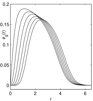
(a).   (b).

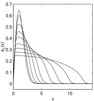
Fig. 5: (a). 2d central vortex states $\phi_{g}(r)$ in Example 5. $\beta=200$. For $m=1,\;2,\;3,\;4,\;5,\;6$ (in the order of decreasing peak). (b). First excited state solution $\phi_{1}(x)$ (an odd function) in Example 6. For $\beta=0,\;3.1371,\;12.5484,\;31.371,\;62.742,\;156.855,\;313.71,\;627.42,\;1254.8$ (in the order of decreasing peak).

From the results in Table 3 and Figure 5b, we can see that the BEFD can be applied directly to compute the first excited states in BEC. Furthermore, we have

$$\lim_{\beta\to+\infty}\ \frac{{E_{\beta}}(\phi_{1})}{{E_{\beta}}(\phi_{g})}=1,\qquad\lim_{\beta\to+\infty}\ \frac{\mu_{1}}{\mu_{g}}=1.$$

These results are confirmed with the results in [8] where the ground and first excited states are computed by directly minimizing the energy functional through the finite element discretization.

5 Conclusions

Energy diminishing of a normalized gradient flow and its discretization are examined, which provides some mathematical justification of the imaginary time integration method used in physical literatures to compute the ground state solution of Bose-Einstein condensation (BEC). Backward Euler centered finite difference (BEFD) and time-splitting sine-spectral (TSSP) method are proposed to discretize the normalized gradient flow. Comparison between the two proposed methods and existing methods shows that BEFD and TSSP are much better for the computation of the BEC ground state solution. Numerical results in 1d, 2d and 3d with different types of potentials used in BEC are reported to demonstrate the effectiveness of the BEFD and TSSP methods. Furthermore, extension of the normalized gradient flow and its BEFD discretization to compute higher excited states with an orthonormalization technique is on-going.

Appendix: BEFD discretization in BEC when $V({\bf x})$ has symmetry

In this appendix, we present detailed BEFD discretizations for the normalized gradient flows in BEC in 2d and 3d when the potential $V({\bf x})$ and the initial data $\phi_{0}({\bf x})$ have symmetry with/without a central vortex state in the condensate. Choose $R>0$, $a<b$ and time step $k>0$ with $|a|$, $b$, $R$ sufficiently large. Denote the mesh size $h_{r}=(R-0)/M$ and $h_{z}=(b-a)/N$ with $M$ and $N$ two positive integers, time steps $t_{n}=n\;k$, $n=0,1,\cdots$, and grid points $r_{j}=j\,h_{r}$, $j=0,1,\cdots,M$ and $r_{j-\frac{1}{2}}=\left(j-\frac{1}{2}\right)h_{r}$, $j=0,1,\cdots,M+1$, $z_{l}=a+l\,h_{z}$, $l=0,1,\cdots,N$.

A1. 2d with radial symmetry and 3d with spherical symmetry, i.e. $V({\bf x})=V(r)$ and $\phi_{0}({\bf x})=\phi_{0}(r)$ with $r=|{\bf x}|$ and $\Omega={\mathbb{R}}^{d}$ with $d=2,3$ in (2.19)-(2.22). In this case, the solution $\phi({\bf x},t)=\phi(r,t)$ and the normalized gradient flow collapses to a 1d problem:

$$\phi_{t}=\frac{1}{2r^{d-1}}\frac{\partial}{\partial r}\left(r^{d-1}\frac{\partial\phi}{\partial r}\right)-V(r)\phi-\beta|\phi|^{2}\phi,\quad 0<r<\infty,\ t_{n}<t<t_{n+1},\qquad$$ (E.1)

$$\phi_{r}(0,t)=0,\qquad\lim_{r\to\infty}\phi(r,t)=0,\qquad t\geq 0,$$ (E.2)

$$\phi(r,t_{n+1})\stackrel{{\scriptstyle\triangle}}{{=}}\frac{\phi(r,t_{n+1}^{-})}{\|\phi(\cdot,t_{n+1}^{-})\|},\qquad 0<r<\infty,\quad n\geq 0,$$ (E.3)

$$\phi(r,0)=\phi_{0}(r)\geq 0,\qquad 0<r<\infty;$$ (E.4)

where $\|\phi_{0}\|=1$ and the norm $\|\cdot\|$ is defined as

$$\|\phi\|^{2}=C_{d}\int_{0}^{\infty}\phi^{2}(r,t)r^{d-1}\;dr.$$

with

$$C_{d}=\left\{\begin{array}[]{ll}2\pi,&\qquad d=2,\\ 4\pi,&\qquad d=3.\\ \end{array}\right.$$

The BEFD discretization of (E.1)-(E.4) is:

$$\frac{\phi_{j-\frac{1}{2}}^{*}-\phi_{j-\frac{1}{2}}^{n}}{k}=\frac{1}{2\;h_{r}^{2}\;r_{j-\frac{1}{2}}^{d-1}}\left[r_{j}^{d-1}\;\phi_{j+\frac{1}{2}}^{*}-\left(r_{j}^{d-1}+r_{j-1}^{d-1}\right)\phi_{j-\frac{1}{2}}^{*}+r_{j-1}^{d-1}\;\phi_{j-\frac{3}{2}}^{*}\right]$$

$$\qquad\qquad-V(r_{j-\frac{1}{2}})\;\phi_{j-\frac{1}{2}}^{*}-\beta\left(\phi_{j-\frac{1}{2}}^{n}\right)^{2}\phi_{j-\frac{1}{2}}^{*},\quad j=1,\cdots,M-1,$$

$$\phi_{-\frac{1}{2}}^{*}=\phi_{\frac{1}{2}}^{*},\qquad\phi_{M-\frac{1}{2}}^{*}=0,$$

$$\phi_{j-\frac{1}{2}}^{n+1}=\frac{\phi_{j-\frac{1}{2}}^{*}}{\|\phi^{*}\|},\qquad j=0,\cdots,M,\qquad n=0,1,\cdots,$$ (E.5)

$$\phi_{j-\frac{1}{2}}^{0}=\phi_{0}(r_{j}),\qquad j=1,\cdots,M,\qquad\phi_{-\frac{1}{2}}^{0}=\phi_{\frac{1}{2}}^{0},$$

where the norm is defined as

$$\|\phi^{*}\|^{2}=h_{r}C_{d}\sum_{j=1}^{M}\left(\phi_{j-\frac{1}{2}}^{*}\right)^{2}\;r_{j-\frac{1}{2}}^{d-1}.$$

A2. 3d with cylindrical symmetry, i.e. $V({\bf x})=V(r,z)$ and $\phi_{0}({\bf x})=\phi_{0}(r,z)$ with $r=\sqrt{x^{2}+y^{2}}$ and $\Omega={\mathbb{R}}^{d}$ with $d=3$ in (2.19)-(2.22). This is the most popular case in the setup of current BEC experiments. In this case, the solution $\phi({\bf x},t)=\phi(r,z,t)$ and the normalized gradient flow collapses to a 2d problem with $0<r<\infty$ and $-\infty<z<\infty$:

$$\phi_{t}=\frac{1}{2}\left[\frac{1}{r}\frac{\partial}{\partial r}\left(r\frac{\partial\phi}{\partial r}\right)+\frac{\partial^{2}\phi}{\partial z^{2}}\right]-V(r,z)\phi-\beta|\phi|^{2}\phi,\quad t_{n}<t<t_{n+1},\qquad$$ (E.6)

$$\phi_{r}(0,z,t)=0,\quad\lim_{r\to\infty}\phi(r,z,t)=0,\quad\lim_{z\to\pm\infty}\phi(r,z,t)=0,\qquad t\geq 0,$$ (E.7)

$$\phi(r,z,t_{n+1})\stackrel{{\scriptstyle\triangle}}{{=}}\frac{\phi(r,z,t_{n+1}^{-})}{\|\phi(\cdot,t_{n+1}^{-})\|},\quad n\geq 0,$$ (E.8)

$$\phi(r,z,0)=\phi_{0}(r,z)\geq 0;$$ (E.9)

where $\|\phi_{0}\|=1$ and the norm $\|\cdot\|$ is defined as

$$\|\phi\|^{2}=2\pi\int_{0}^{\infty}\int_{-\infty}^{\infty}\phi^{2}(r,z,t)r\;dzdr.$$

The BEFD discretization of (E.6)-(E.9) is:

$$\frac{\phi_{j-\frac{1}{2}\,l}^{*}-\phi_{j-\frac{1}{2}\,l}^{n}}{k}=\frac{1}{2\;h_{r}^{2}\;r_{j-\frac{1}{2}}}\left[r_{j}\;\phi_{j+\frac{1}{2}\,l}^{*}-\left(r_{j}+r_{j-1}\right)\phi_{j-\frac{1}{2}\,l}^{*}+r_{j-1}\;\phi_{j-\frac{3}{2}\,l}^{*}\right]$$

$$\qquad\qquad+\frac{1}{2h_{z}^{2}}\left[\phi_{j-\frac{1}{2}\,l+1}^{*}-2\phi_{j-\frac{1}{2}\,l}^{*}+\phi_{j-\frac{1}{2}\,l-1}^{*}\right]-V(r_{j-\frac{1}{2}},z_{l})\;\phi_{j-\frac{1}{2}\,l}^{*}$$

$$\qquad\qquad-\beta\left(\phi_{j-\frac{1}{2}\,l}^{n}\right)^{2}\;\phi_{j-\frac{1}{2}\,l}^{*},\quad j=1,\cdots,M-1,\quad l=1,2\cdots,N-1,$$

$$\phi_{-\frac{1}{2}\,l}^{*}=\phi_{\frac{1}{2}\,l}^{*},\quad\phi_{M-\frac{1}{2}\,l}^{*}=0,\quad l=1,2,\cdots,N-1,$$

$$\phi_{j-\frac{1}{2}\,0}^{*}=\phi_{j-\frac{1}{2}\,M}^{*}=0,\quad j=0,1,\cdots,M.$$

$$\phi_{j-\frac{1}{2}\,l}^{n+1}=\frac{\phi_{j-\frac{1}{2}\,l}^{*}}{\|\phi^{*}\|},\quad j=0,\cdots,M,\quad l=0,1,\cdots,N,\quad n=0,1,\cdots,\qquad$$ (E.10)

$$\phi_{j-\frac{1}{2}\,l}^{0}=\phi_{0}(r_{j-\frac{1}{2}},z_{l}),\qquad j=1,\cdots,M,\quad l=0,\cdots,N,$$

$$\phi_{-\frac{1}{2}\,l}^{0}=\phi_{\frac{1}{2}\,l}^{0},\quad l=0,1,\cdots,N,$$

where the norm is defined as

$$\|\phi^{*}\|^{2}=2\pi h_{r}h_{z}\sum_{j=1}^{M}\sum_{l=1}^{N-1}\left(\phi_{j-\frac{1}{2}\,l}^{*}\right)^{2}\;r_{j-\frac{1}{2}}.$$

In finding a stationary solution of (1.1) with a central vortex state, one plugs the ansatz

$$\psi({\bf x},t)=\left\{\begin{array}[]{ll}e^{-i\mu t}\;e^{im\theta}\;\phi(r),&\qquad d=2,\\ e^{-i\mu t}\;e^{im\theta}\;\phi(r,z),&\qquad d=3,\\ \end{array}\right.\qquad r=\sqrt{x^{2}+y^{2}}$$

into (1.1) instead of (1.5), where $m>0$ an integer corresponding to the index of the vortex. For more details related to central vortex states in BEC, we refer [18, 29, 34, 36].

A3. 2d central vortex states in BEC, i.e. $V({\bf x})=V(r)=\frac{1}{2}\left(\frac{m^{2}}{r^{2}}+r^{2}\right)$ and $\phi_{0}({\bf x})=\phi_{0}(r)with\phi_{0}(0)=0$, $r=\sqrt{x^{2}+y^{2}}$ and $\Omega={\mathbb{R}}^{2}$ in (2.19)-(2.22). In this case, the solution $\phi({\bf x},t)=\phi(r,t)$ and the normalized gradient flow collapses to a 1d problem:

$$\phi_{t}=\frac{1}{2r}\frac{\partial}{\partial r}\left(r\frac{\partial\phi}{\partial r}\right)-V(r)\phi-\beta|\phi|^{2}\phi,\quad 0<r<\infty,\quad t_{n}<t<t_{n+1},\qquad$$ (E.11)

$$\phi(0,t)=0,\qquad\lim_{r\to\infty}\phi(r,t)=0,\qquad t\geq 0,$$ (E.12)

$$\phi(r,t_{n+1})\stackrel{{\scriptstyle\triangle}}{{=}}\frac{\phi(r,t_{n+1}^{-})}{\|\phi(\cdot,t_{n+1}^{-})\|},\qquad 0<r<\infty,\quad n\geq 0,$$ (E.13)

$$\phi(r,0)=\phi_{0}(r)\geq 0,\quad 0<r<\infty,\qquad\left({\rm e.g.}=\frac{1}{\sqrt{\pi m!}}\;r^{m}\;e^{-r^{2}/2}\right);$$ (E.14)

where $\phi(0)=0$, $\|\phi_{0}\|=1$ and the norm $\|\cdot\|$ is defined as

$$\|\phi\|^{2}=2\pi\int_{0}^{\infty}\phi^{2}(r,t)r\;dr.$$

The BEFD discretization of (E.11)-(E.14) is:

$$\frac{\phi_{j}^{*}-\phi_{j}^{n}}{k}=\frac{1}{2\;h_{r}^{2}\;r_{j}}\left[r_{j+\frac{1}{2}}\;\phi_{j+1}^{*}-\left(r_{j+\frac{1}{2}}+r_{j-\frac{1}{2}}\right)\phi_{j}^{*}+r_{j-\frac{1}{2}}\;\phi_{j-1}^{*}\right]$$

$$\qquad\qquad-V(r_{j})\;\phi_{j}^{*}-\beta\left(\phi_{j}^{n}\right)^{2}\phi_{j}^{*},\quad j=1,\cdots,M-1,$$

$$\phi_{0}^{*}=\phi_{M}^{*}=0,$$

$$\phi_{j}^{n+1}=\frac{\phi_{j}^{*}}{\|\phi^{*}\|},\qquad j=0,\cdots,M,\qquad n=0,1,\cdots,$$ (E.15)

$$\phi_{j}^{0}=\phi_{0}(r_{j}),\qquad j=0,1,\cdots,M,$$

where the norm is defined as

$$\|\phi^{*}\|^{2}=2\pi h_{r}\sum_{j=1}^{M-1}r_{j}\;\left(\phi_{j}^{*}\right)^{2}.$$

A4. 3d central vortex states in BEC, i.e. $V({\bf x})=V(r,z)=\frac{1}{2}\left(\frac{m^{2}}{r^{2}}+\gamma_{r}^{2}r^{2}+\gamma_{z}^{2}z^{2}\right)$ and $\phi_{0}({\bf x})=\phi_{0}(r,z)$ with $\phi_{0}(0,z)=0$ for $z\in{\mathbb{R}}$, $\gamma_{r}>0$, $\gamma_{z}>0$ constants, $r=\sqrt{x^{2}+y^{2}}$ and $\Omega={\mathbb{R}}^{3}$ in (2.19)-(2.22). In this case, the solution $\phi({\bf x},t)=\phi(r,z,t)$ and the normalized gradient flow collapses to a 2d problem with $0<r<\infty$ and $-\infty<z<\infty$:

$$\phi_{t}=\frac{1}{2}\left[\frac{1}{r}\frac{\partial}{\partial r}\left(r\frac{\partial\phi}{\partial r}\right)+\frac{\partial^{2}\phi}{\partial z^{2}}\right]-V(r,z)\phi-\beta\phi^{3},\quad t_{n}<t<t_{n+1},\qquad$$ (E.16)

$$\phi(0,z,t)=0,\quad\lim_{r\to\infty}\phi(r,z,t)=0,\quad\lim_{z\to\pm\infty}\phi(r,z,t)=0,\qquad t\geq 0,$$ (E.17)

$$\phi(r,z,t_{n+1})\stackrel{{\scriptstyle\triangle}}{{=}}\frac{\phi(r,z,t_{n+1}^{-})}{\|\phi(\cdot,t_{n+1}^{-})\|},\quad n\geq 0,$$ (E.18)

$$\phi(r,z,0)=\phi_{0}(r,z)\geq 0,\qquad\left({\rm e.g.}=\frac{\gamma_{z}^{1/4}\gamma_{r}^{(m+1)/2}}{\pi^{3/4}(m!)^{1/2}}r^{m}\;e^{-(\gamma_{r}r^{2}+\gamma_{z}z^{2})/2}\right);\qquad\quad$$ (E.19)

where $\phi_{0}(0,z)=0$ for $z\in{\mathbb{R}}$, $\|\phi_{0}\|=1$ and the norm $\|\cdot\|$ is defined as

$$\|\phi\|^{2}=2\pi\int_{0}^{\infty}\int_{-\infty}^{\infty}\phi^{2}(r,z,t)r\;dzdr.$$

The BEFD discretization of (E.16)-(E.19) is:

$$\frac{\phi_{j\,l}^{*}-\phi_{j\,l}^{n}}{k}=\frac{1}{2\;h_{r}^{2}\;r_{j}}\left[r_{j+\frac{1}{2}}\;\phi_{j+1\,l}^{*}-\left(r_{j+\frac{1}{2}}+r_{j-\frac{1}{2}}\right)\phi_{j\,l}^{*}+r_{j-\frac{1}{2}}\;\phi_{j-1\,l}^{*}\right]$$

$$\qquad\qquad+\frac{1}{2h_{z}^{2}}\left[\phi_{j\,l+1}^{*}-2\phi_{j\,l}^{*}+\phi_{j\,l-1}^{*}\right]-V(r_{j},z_{l})\;\phi_{j\,l}^{*}-\beta\left(\phi_{j\,l}^{n}\right)^{2}\phi_{j\,l}^{*},$$

$$\qquad\qquad\quad j=1,\cdots,M-1,\ l=1,2\cdots,N-1,$$

$$\phi_{0\,l}^{*}=\phi_{M\,l}^{*}=0,\quad l=0,1,\cdots,N,\quad\phi_{j\,0}^{*}=\phi_{j\,M}^{*}=0,\quad j=1,1,\cdots,M-1.$$

$$\phi_{j\,l}^{n+1}=\frac{\phi_{j\,l}^{*}}{\|\phi^{*}\|},\quad j=0,\cdots,M,\quad l=0,1,\cdots,N,\quad n=0,1,\cdots,\qquad$$ (E.20)

$$\phi_{j\,l}^{0}=\phi_{0}(r_{j},z_{l}),\qquad j=0,\cdots,M,\quad l=0,\cdots,N,$$

where the norm is defined as

$$\|\phi^{*}\|^{2}=2\pi h_{r}h_{z}\sum_{j=1}^{M-1}\sum_{l=1}^{N-1}\left(\phi_{j\,l}^{*}\right)^{2}\;r_{j}.$$

The linear system at every time step in A1 and A3 can be solved by the Thomas algorithm and in A2 and A4 can be solved by Gauss-Seidel iterative method.

a).   b)

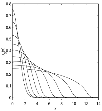
a).   b).

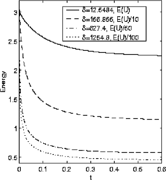
Fig. 2: Ground state solution $\phi_{g}(x)$ (labeled as $u_{g}$) in Example 2. (a). For $\beta=0,\;3.1371,\;12.5484,\;31.371,\;62.742,\;156.855,\;313.71,\;627.42,\;1254.8$ (in the order of decreasing peak). (b). Energy evolution for different $\beta$ (labeled as $\delta$).

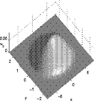
(a).   (b).

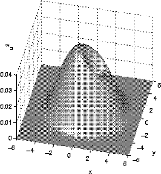
Fig. 3: Surface plots of the ground state solutions $\phi_{g}^{2}(x,y)$ (labeled as $u^{2}$) in Example 3, case I (a), and case II (b).

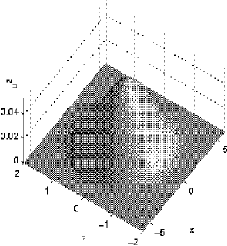
a).   b).

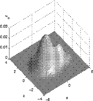
Fig. 4: Surface plots of the ground state solutions $\phi_{g}^{2}(x,0,z)$ (labeled as $u^{2}$) in Example 4. (a). For case I. (b). For case II.

References

- [1] S.K. Adhikari, Numerical solution of the two-dimensional Gross-Pitaevskii equation for trapped interacting atoms, Phys. Lett. A, 265(2000), pp. 91-96.
- [2] S.K. Adhikari, Numerically study of the spherically symmetric Gross-Pitaevskii equation in two space dimensions, Phys. Rev. E, 62(2000), pp. 2937-2944.
- [3] A. Aftalion A, and Q. Du, Vortices in a rotating Bose-Einstein condensate: Critical angular velocities and energy diagrams in the Thomas-Fermi regime, Phys. Rev. A, 64(2001), pp. 063603.
- [4] M.H. Anderson, J.R. Ensher, M.R. Matthews, C.E. Wieman, and E.A. Cornell, Observation of Bose-Einstein condensation in a dilute atomic vapor, Science, 269(1995), pp. 198-201.
- [5] J.R. Anglin and W. Ketterle, Bose-Einstein condensation of atomic gases, Nature, 416(2002), pp. 211-218.
- [6] W. Bao, S. Jin and P.A. Markowich, On time-splitting spectral approximations for the Schrödinger equation in the semiclassical regime, J. Comput. Phys., 175(2002), pp. 487-524.
- [7] W. Bao, S. Jin and P.A. Markowich, Numerical study of time-splitting spectral discretizations of nonlinear Schrödinger equations in the semi-clasical regimes, SIAM J. Sci. Comp., to appear.
- [8] W. Bao and W. Tang, Ground state solution of trapped interacting Bose-Einstein condensate by directly minimizing the energy functional, J. Comput. Phys., to appear.
- [9] W. Bao, D. Jaksch and P.A. Markowich, Numerical solution of the Gross-Pitaevskii equation for Bose-Einstein condensation, J. Comput. Phys., to appear.
- [10] W. Bao, D. Jaksch, An explicit unconditionally stable numerical methods for solving damped nonlinear Schrodinger equations with a focusing nonlinearity, SIAM J. Numer. Anal., to appear.
- [11] B.M. Caradoc-Davis, R.J. Ballagh and K. Burnett, Coherent dynamics of vortex formation in trapped Bose-Einstein condensates, Phys. Rev. Lett., 83(1999), pp. 895.
- [12] B.M. Caradoc-Davis, R.J. Ballagh and P.B. Blakie, Three-dimensional vortex dynamics in Bose-Einstein condensates, Phys. Rev. A, 62(2000), pp. 011602.
- [13] M.M. Cerimele, M.L. Chiofalo, F. Pistella, S. Succi and M.P. Tosi, Numerical solution of the Gross-Pitaevskii equation using an explicit finite-difference scheme: An application to trapped Bose-Einstein condensates, Phys. Rev. E, 62(2000), pp. 1382-1389.
- [14] M.M. Cerimele, F. Pistella and S. succi, Particle-inspired scheme for the Gross-Pitaevski equation: An application to Bose-Einstein condensation, Comput. Phys. Comm., 129(2000), pp. 82-90.
- [15] M.L. Chiofalo, S. Succi and M.P. Tosi, Ground state of trapped interacting Bose-Einstein condensates by an explicit imaginary-time algorithm, Phys. Rev. E, 62(2000), pp. 7438-7444.
- [16] E. Cornell, Very cold indeed: The nanokelvin physics of Bose-Einstein condensation, J. Res. Natl. Inst. Stan., 101(1996), pp. 419-434.
- [17] F. Dalfovo, S. Giorgini, L.P. Pitaevskii and S. Stringari, Rev. Mod. Phys., 71(1999), 463.
- [18] F. Dalfovo and S. Stringari, Bosons in anisotropic traps: Ground state and vortices, Phys. Rev. A, 53(1996), pp. 2477-2485.
- [19] R.J. Dodd, Approximate solutions of the nonlinear Schrödinger equation for ground and excited states of Bose-Einstein condensates, J. Res. Natl. Inst. Stan., 101(1996), pp. 545-552.
- [20] Q. Du, Numerical computations of quantized vortices in Bose-Einstein condensate, in Recent Progress in computational and applied PDEs, edited by T. Chan et. al., Kluwer Academic Publisher, pp.155-168, 2002.
- [21] M. Edwards and K. Burnett, Numerical solution of the nonlinear Schrödinger equation for small samples of trapped neutral atoms, Phys. Rev. A, 51(1995), pp. 1382-1386.
- [22] G. Fibich and G. Papanicolaou, Self-focusing in the perturbed and unperturbed nonlinear Schrödinger equation in critical dimension, SIAM J. Appl. Math., 60(2000), pp. 183-240.
- [23] A. Gammal, T. Frederico and L. Tomio, Improved numerical approach for the time-independent Gross-Pitaevskii nonlinear Schrödinger equation, Phys. Rev. E, 60(1999), pp. 2421-2424.
- [24] G.H. Golub and C.F. Van Loan, Matrix computations, Johns Hopkins University Press, 1989.
- [25] M. Greiner, O. Mandel, T. Esslinger, T.W. Hänsch, and I. Bloch, Quantum phase transition from a superfluid to a mott insulator in a gas of ultracold atoms, Nature, 415(2002), pp. 39-45.
- [26] E.P. Gross, Nuovo. Cimento., 20(1961), pp. 454.
- [27] B. Jackson, J.F. McCann and C.S. Adams, Vortex formation in dilute inhomogeneous Bose-Einstein condensates, Phys. Rev. Lett., 80 (1998), pp. 3903-3906.
- [28] D. Jaksch, C. Bruder, J. I. Cirac, C. W. Gardiner, and P. Zoller, Cold bosonic atoms in optical lattices, Phys. Rev. Lett., 81(1998), pp. 3108-3111.
- [29] V. V. Konotop and V. M.Pérez-García, Solutions of Gross-Pitaevskii equations beyond the hydrodynamics approximation: Applicaiton to the vortex problem, Pyhs. Rev. A, 62(2000), pp. 033610: 1-7.
- [30] L. Landau and E. Lifschitz, Quantum Mechanics: non-relativistic theory, Pergamon Press, New York, 1977.
- [31] I. N. Levine, Quantum Chemistry (Fifth Edition) (Prentice Hall International, Inc., New York, 1991).
- [32] E.H. Lieb, R. Seiringer and J. Yngvason, Bosons in a Trap: A Rigorous Derivation of the Gross-Pitaevskii Energy Functional, Phys. Rev. A, 61(2000), pp. 3602.
- [33] F. Lin and Q. Du, Ginzburg-Landau vortices: dynamics, pinning, and hysteresis, SIAM J. Math. Anal., 28(1997), pp. 1265-1293.
- [34] E. Lundh, C.J. Pethick and H. Smith, Vortics in Bose-Einetein-condensated atomic clouds, Phys. Rev. A, 59 (1998), pp. 4816-4823.
- [35] L.P. Pitaevskii, Zh. Eksp. Teor. Fiz., 40(1961), pp. 646. (Sov. Phys. JETP, 13(1961), pp. 451).
- [36] D.S. Rokhsar, Vortex stability and persistent currents in trapped Bose gas, Phys. Rev. Lett., 79(1997), pp 2164-2167.
- [37] P.A. Ruprecht, M.J. Holland, K. Burrett and M. Edwards, Time-dependent solution of the nonlinear Schrödinger equation for Bose-condensed trapped neutral atoms, Phys. Rev. A, 51(1995), pp. 4704-4711.
- [38] B.I. Schneider and D.L. Feder, Numerical approach to the ground and excited states of a Bose-Einstein condensated gas confined in a completely anisotropic trap, Phys. Rev. A, 59(1999), pp. 22332-2242.
- [39] L. Simon, Asymptotics for a class of nonlinear evolution equations, with applications to geometric problems, Annals of Math., 118(1983), pp. 525-571.
- [40] C. Sulem and P.L. Sulem, The Nonlinear Schrödinger Equation: Self-focusing and Wave Collapse, Springer, New York, 1999.
a). b)
b)
c). d)
d)
e). f)
f)
a). b).
b).
(a). (b).
(b).
a). b).
b).
(a).  (b).
(b).