Upper critical field in dirty two-band superconductors: breakdown of the anisotropic Ginzburg-Landau theory

Abstract

We investigate the upper critical field in a dirty two-band superconductor within quasiclassical Usadel equations. The regime of very high anisotropy in the quasi-2D band, relevant for MgB₂, is considered. We show that strong disparities in pairing interactions and diffusion constant anisotropies for two bands influence the in-plane $H_{c2}$ in a different way at high and low temperatures. This causes temperature-dependent $H_{c2}$ anisotropy, in accordance with recent experimental data in MgB₂. The three-dimensional band most strongly influences the in-plane $H_{c2}$ near $T_{c}$, in the Ginzburg-Landau (GL) region. However, due to a very large difference between the c-axis coherence lengths in the two bands, the GL theory is applicable only in an extremely narrow temperature range near $T_{c}$. The angular dependence of $H_{c2}$ deviates from a simple effective-mass law even near $T_{c}$.

I Introduction

There is a strong evidence of the multigap nature of superconducting state in the recently discovered Akimitsu compound MgB₂. The concept of multiband superconductivity was introduced in Suhl ; Moskal for the case of large disparity of the electron-phonon interaction for the different Fermi-surface sheets. For MgB₂, first-principles calculations of the electronic structure and the electron-phonon interaction Kortus ; An ; LiuPRL01 ; Shulga ; Kong ; Yildirim have revealed two distinct groups of bands, namely strongly superconducting quasi-two-dimensional $\sigma$-bands and weakly superconducting three-dimensional $\pi$-bands. Quantitative predictions for various thermodynamic and transport properties of MgB₂ were made in the framework of the two-band model. Choi ; Golub ; Brink ; Mazin02

A large number of experimental data, in particular tunneling, GiubileoPRL01 ; IavaronePRL02 point contact measurements,SzaboPRL01 ; SchmidtPRL01 ; Gonnelli and heat capacity measurements,BouquetPRL01 directly support the concept of a double gap MgB₂. Intraband impurity scattering in both bands may vary in large limits, while interband scattering is always weak due to the disparity of $\sigma$- and $\pi$-band wave functions.Mazin02 This explains the extremely weak suppression of $T_{c}$ by impurities and the weak correlation between $T_{c}$ and the resistivity. Therefore, a unique feature of the MgB₂ is that the two-gap nature of superconductivity persists even in the dirty limit for the intraband scattering rates.

Superconductivity in the two bands is characterized by different energy and length scales which show up in several properties of a superconductor. Particularly interesting are the properties of the mixed state. The c-axis Abrikosov vortex structure in MgB₂ was studied by STM in Ref. Eskildsen02, , which probes mainly the weakly superconducting $\pi$-band. A large vortex core size compared to estimates based on $H_{c2}$ and the rapid suppression of the apparent tunneling gap by small magnetic fields has been reported. These observations can be naturally explained within the two-band model.Nakai ; KG

One of the most spectacular consequences of the two-band superconductivity is the unusual behavior of anisotropy factors for different physical parameters.KoganBudko It was demonstrated that in clean MgB₂ samples the anisotropy of the London penetration depth,Kogan_lam ; Golub_lam $\gamma_{\lambda}$, has to be very different from the anisotropy of the upper critical field,Kogan ; Dahm $\gamma_{c2}$. Both anisotropy factors should strongly depend on temperature and have opposite temperature dependencies: $\gamma_{\lambda}$ is expected to increase and $\gamma_{c2}$ is expected to decrease with temperature. Strong temperature dependence of $\gamma_{c2}$ has been reliably confirmed by experiment.Sologub ; Budko ; Angst ; Eltsev ; Lyard ; WelpPRB03 Typically, $\gamma_{c2}$ drops from 5-6 at low temperatures down to $\sim$ 2 near $T_{c}$.

In this paper we consider in detail the behavior of the upper critical field for different field orientations for the case of a dirty two-band superconductor with weak interband scattering. The model is based on the multiband generalization of the quasiclassical Usadel equations.Usadel The same model has been used recently to describe vortex core structure in MgB₂.KG The general equations for determination of the upper critical field within this model have been derived in recent paper Gurevich, . However, calculations in this paper have been done only for the case of small band anisotropies. In this paper we address the case of very high anisotropy in the quasi-2D band, more suitable for MgB₂.

We demonstrate that the strong temperature dependence of the $H_{c2}$-anisotropy exists also in the dirty case and therefore represents a general property of a two-band superconductor. The main reason for this dependence is the strong reduction of the in-plane upper critical field by the weak $\pi$-band in the very narrow temperature region near $T_{c}$. This also leads to the significant upward curvature of the temperature dependence of the in-plane upper critical field near $T_{c}$. This behavior illustrates breakdown of the anisotropic Ginzburg-Landau (GL) theory for description of this superconductor. We demonstrate that, due to the large difference between microscopic coherence lengths in the c-direction for the two bands, the anisotropic GL theory is applicable only within the extremely narrow temperature range near $T_{c}$.

We analyze the angular dependence of the upper critical field and show that it strongly deviates from the standard “effective-mass” dependence predicted by the anisotropic GL theory. Contrary to naive expectations, these deviations are strongest for temperatures quite close to $T_{c}$ (at $T\sim 0.9T_{c}$) and vanish only for temperatures extremely close to $T_{c}$ (for $(T_{c}-T)/T_{c}\lesssim 1\%$). In the past the angular dependence of the upper critical field have been studied in Ref. Langmann, for a clean two-band superconductor. It was shown that for the case of two weakly deformed spherical Fermi surfaces with opposite anisotropies the angular dependence also strongly deviates from the “effective-mass” law.

The paper is organized as follows. In section II we present Usadel equations for a two-band superconductor and introduce parameters relevant for MgB₂. In section III we derive equation for the upper critical field in the c-direction and obtain the exact asymptotics at small and high temperatures. In section IV we consider the in-plane upper critical field. We derive general equations for determination of this field and study solutions of these equations in different regimes. We demonstrate that the GL result for the in-plane $H_{c2}$ is valid only within a very narrow range of temperatures. We also numerically calculate in-plane $H_{c2}$ and the anisotropy parameter $\gamma_{c2}$ in the whole temperature range. In section V we study the angular dependence of the upper critical field and analyze quantitatively the deviations from the effective-mass law.

II The model: Usadel equations for a two-band superconductor

We consider a two-band superconductor with weak interband impurity scattering and rather strong intraband scattering rates exceeding the corresponding energy gaps (dirty limit). In this case the quasiclassical Usadel equations Usadel are applicable within each band. The mixed state in this case is described by the system of coupled Usadel equations Usadel ; KG

$$\omega F_{\alpha}\! -\!\sum_{j}\frac{\mathcal{D}_{\alpha,j}}{2}\left[G_{\alpha}(\nabla_{j}\!-\!\frac{2\pi i}{\Phi_{0}}A_{j})^{2}F_{\alpha}\!-\!F_{\alpha}\nabla_{j}^{2}G_{\alpha}\right]$$

$$=\Delta_{\alpha}G_{\alpha},$$ (1a)

$$\Delta_{\alpha} =2\pi T\sum_{\beta,n}\Lambda_{\alpha\beta}F_{\beta},$$ (1b)

where $\alpha=1,2$ is the band index, $j=x,y,z$ is the coordinate index, $\hat{\Lambda}$ is the matrix of effective coupling constants, $\mathcal{D}_{\alpha,j}$ are diffusion constants, which determine the coherence lengths $\xi_{\alpha,j}=\sqrt{\mathcal{D}_{\alpha,j}/2\pi T_{c}}$, $G_{\alpha},$ $F_{\alpha}$ and $\Delta_{\alpha}$ are normal and anomalous Green’s functions and the pair potential, respectively, and $\omega=2\pi T(s+1/2)$ are Matsubara frequencies. Bearing in mind the application to MgB₂, in our notations index 1 corresponds to $\sigma$-bands and index 2 to $\pi$-bands. All bands are isotropic in the $xy$ plane, $\mathcal{D}_{\alpha x}=\mathcal{D}_{\alpha y}$ and anisotropic in the $xz$ plane with the anisotropy ratios $\gamma_{\alpha}=\sqrt{\mathcal{D}_{\alpha x}/\mathcal{D}_{\alpha z}}$. The multigap Usadel equations for general case, taking into account also interband scattering, have been recently derived in Ref. Gurevich, .

The selfconsistency equation can be rewritten in the form

$$\!W_{1}\Delta_{1}\!-W_{12}\Delta_{2}\!= 2\pi T\!\sum_{\omega>0}\!\left(F_{1}\!-\frac{\Delta_{1}}{\omega}\right)\!+\Delta_{1}\ln\frac{T_{c}}{T},$$ (2a)

$$\!-W_{21}\Delta_{1}\!+\!W_{2}\Delta_{2}\!\!= 2\pi T\!\sum_{\omega>0}\!\left(F_{2}\!-\frac{\Delta_{2}}{\omega}\!\right)\!+\!\Delta_{2}\ln\frac{T_{c}}{T},$$ (2b)

with the following matrix $$W_{\alpha\beta}$$

$$W_{1} \!=\frac{-A+\sqrt{A^{2}+\Lambda_{12}\Lambda_{21}}}{\mathrm{Det}},\ W_{2}\!=\frac{A+\sqrt{A^{2}+\Lambda_{12}\Lambda_{21}}}{\mathrm{Det}},$$

$$W_{12} =\Lambda_{12}/\mathrm{Det},\ W_{21}=\Lambda_{21}/\mathrm{Det,}$$ (3)

$A=(\Lambda_{11}-\Lambda_{22})/2,$ $\mathrm{Det}=\Lambda_{11}\Lambda_{22}-\Lambda_{12}\Lambda_{21}$, $W_{1}W_{2}=W_{12}W_{21}$.

The electron-phonon interaction in MgB₂ was calculated from first principles in a number of papers.LiuPRL01 ; Choi ; Golub Here we use the effective coupling constants $\Lambda_{ij}$ from Ref. Golub, : $\!\Lambda_{11}\!\approx 0.81,\ \Lambda_{22}\!\approx 0.278,\ \Lambda_{12}\!\approx 0.115,\ \Lambda_{21}\!\approx 0.091,$ from which we obtain values of $W_{\alpha\beta}$ used in numerical calculations,

$$\!W_{1}\!\approx 0.088,\ W_{2}\!\approx 2.56,\ W_{12}\!\approx 0.535,\ W_{21}\!\approx 0.424.$$ (4)

The relative role of the weak band is characterized by the ratio $S_{12}\equiv W_{1}\!/W_{2}$,Parameters which in the case of MgB₂ is rather small, $S_{12}\approx 0.034$. This ratio will be used below as a small parameter in our model to derive various approximations for the upper critical field. Another important small parameter is the ratio of diffusion coefficients in the $\sigma$-band, $\mathcal{D}_{1z}/\mathcal{D}_{1x}$. We will show in this paper that these two parameters, $S_{12}$ and $\mathcal{D}_{1z}/\mathcal{D}_{1x},$ influence differently $H_{c2}$ for parallel field at high and low temperatures thus causing the temperature dependence of the anisotropy.

In the following we consider separately the cases when the field is parallel and perpendicular to the ab-plane.

III Field in the $c$-direction

Let us first study the case when the magnetic field is oriented along c-axis. The upper critical field is determined by the linearized Usadel equation

$$\omega F_{\alpha}+\frac{\mathcal{D}_{\alpha x}}{2}\left(-\nabla_{x}^{2}F_{\alpha}+\left(\frac{2\pi Hx}{\Phi_{0}}\right)^{2}F_{\alpha}\right)=\Delta_{\alpha}$$ (5)

and selfconsistency equations (2). Solving these equations, we arrive at the equation for $H_{c2}^{\perp}$ (symbol $\perp$ denotes the field direction perpendicular to the (ab)- plane)

$$\ln\frac{1}{t}-g\left(\frac{H_{c2}^{\perp}}{tH_{1}}\right)=-\frac{W_{1}\left(\ln\frac{1}{t}-g\left(\frac{H_{c2}^{\perp}}{tH_{2}}\right)\right)}{W_{2}-\left(\ln\frac{1}{t}-g\left(\frac{H_{c2}^{\perp}}{tH_{2}}\right)\right)},$$ (6)

where $t=T/T_{c}$, $H_{\alpha}\equiv 2T_{c}\Phi_{0}/\mathcal{D}_{\alpha x}$, $g(x)=\psi(1/2+x)-\psi(1/2)$, and $\psi(x)$ is a digamma function. We also obtain a relation between $\Delta_{01}$ and $\Delta_{02}$ near $H_{c2}^{\perp}$

$$\Delta_{02}=\frac{W_{21}\Delta_{01}}{W_{2}-\ln\frac{1}{t}+g\left(\frac{H_{c2}^{\perp}}{tH_{2}}\right)}.$$ (7)

In the absence of coupling to the weak $\pi$-band ($W_{1}=0$) or in the case of identical diffusion constants ($\mathcal{D}_{1x}=\mathcal{D}_{2x}$), the upper critical field $H_{c2}^{s}$ is given by the standard Maki - de Gennes equation MakiHc2 ; deGennesHc2

$$\ln(1/t)=g\left[H_{c2}^{s}/(tH_{1})\right].$$ (8)

The well-known asymptotic solutions of this equation at low and high temperatures are respectively

$$\frac{H_{c2}^{s}(t)}{H_{1}}=\left\{\begin{array}[c]{c}e^{-\gamma_{E}}/4\approx 0.140,\text{ }t\ll 1,\\ 2(1-t)/\pi^{2}\approx 0.203(1-t),\text{ }1-t\ll 1,\end{array}\right.$$ (9)

where $\gamma_{E}\approx 0.577$ is Euler constant. In the temperature range near $T_{c}$ one can obtain from Eq. (6) the following simple expression for $H_{c2}^{\perp}$ for arbitrary ratio $S_{12}\equiv W_{1}/W_{2}$:

$$\frac{H_{c2}^{\perp}}{H_{1}}=\frac{2\left(1+S_{12}\right)(1-t)}{\pi^{2}\left(1+S_{12}\mathcal{D}_{2x}/\mathcal{D}_{1x}\right)}.$$ (10)

At small temperatures, $T\ll T_{c}$, Eq. (6) also has an exact solution (see also Ref. Gurevich, )

$$H_{c2}(0)=H_{c2}^{s}(0)\exp\left(-\frac{W_{1}+W_{2}-\ln\left(r_{x}\right)}{2}+\sqrt{\frac{\left(W_{1}+W_{2}-\ln\left(r_{x}\right)\right)^{2}}{4}+W_{1}\ln\left(r_{x}\right)}\right)$$ (11)

with $r_{x}\equiv\mathcal{D}_{1x}/\mathcal{D}_{2x}$. For MgB₂ the parameter $W_{1}$ is small and typically the inequality $W_{1}\ln\left(r_{x}\right)\ll\left(W_{2}-\ln\left(r_{x}\right)\right)^{2}/4$ is valid. In this case we can expand Eq. (11) with respect to $W_{1}$ and obtain a much simpler result

$$H_{c2}(0)\approx H_{c2}^{s}(0)\left(1+\frac{W_{1}\ln\left(\mathcal{D}_{1x}/\mathcal{D}_{2x}\right)}{W_{2}-\ln\left(\mathcal{D}_{1x}/\mathcal{D}_{2x}\right)}\right).$$ (12)

The $\pi$-band strongly influences the upper critical field only if it is very dirty, $\mathcal{D}_{2x}\ll\mathcal{D}_{1x}\exp(-W_{2})$. In this limit we obtain GurevichError

$$H_{c2}(0)\approx H_{c2}^{(2)}(0)\exp\left(-W_{2}\right)$$

with $H_{c2}^{(2)}(0)\equiv(\exp(-\gamma_{E})/4)H_{2}$.

For the case $W_{1}\ll W_{2}$ realized in MgB₂, the upper critical field is typically determined by the strong band (except for the limit of very small diffusivity $\mathcal{D}_{2x}$ in the second band). A small correction due to the weak band can be found from Eq. (6) using an expansion with respect to the small parameter $S_{12}\equiv W_{1}/W_{2}$. In particular, we found very simple expressions for the slope of $H_{c2}$ at $T_{c}$ and $H_{c2}(0)$:

$$\frac{dH_{c2}}{dT} \approx\frac{dH_{c2}^{s}}{dT}\left(1+S_{12}\frac{\mathcal{D}_{1x}-\mathcal{D}_{2x}}{D_{1x}}\right),$$ (13a)

$$H_{c2}(0) \approx H_{c2}^{s}(0)\left(1+S_{12}\ln\frac{\mathcal{D}_{1x}}{\mathcal{D}_{2x}}\right).$$ (13b)

The signs of the above corrections to the universal curve following from Eq. (8) are positive if $$D_{2x}<D_{1x} D_{2x}>D_{1x}$$ and negative for .

IV Field in the $a$ -direction

IV.1 General relations

The upper critical field in the $a$-direction ($\equiv y$-direction) is determined by the linear equations for the Green’s functions $F_{\alpha}$ in two bands

$$\omega F_{\alpha}-\frac{\mathcal{D}_{\alpha x}}{2}\nabla_{x}^{2}F_{\alpha}+\frac{\mathcal{D}_{\alpha z}}{2}\left(\frac{2\pi Hx}{\Phi_{0}}\right)^{2}F_{\alpha}=\Delta_{\alpha}$$ (14)

with $\omega=2\pi T(s+1/2)$ and the self-consistency conditions (2). A technical difficulty of this problem is that, due to the difference in the anisotropy factors for the two bands, $\gamma_{\alpha}$, the harmonic oscillator operators in Eq. (14) have unmatching sets of eigenstates. We will use an expansion with respect to the eigenfunctions (Landau levels) of the strong [1st] band, $\Psi_{n}(x)$, which are defined as solutions of the oscillator equation

$$\frac{\mathcal{D}_{1z}}{2}\left(\frac{2\pi H}{\Phi_{0}}\right)^{2}x^{2}\Psi_{n}-\frac{\mathcal{D}_{1x}}{2}\nabla_{x}^{2}\Psi_{n}=\varepsilon_{n}\Psi_{n}.$$ (15)

In particular, the eigenvalues $\varepsilon_{n}$ and ground state eigenfunction are given by

$$\varepsilon_{n} =\sqrt{\mathcal{D}_{1z}\mathcal{D}_{1x}}\frac{2\pi H}{\Phi_{0}}\left(n+1/2\right),\$$ (16)

$$\Psi_{0}(x) =\left(\frac{2H}{\gamma_{1}\Phi_{0}}\right)^{1/4}\exp\left(-\frac{\pi Hx^{2}}{\gamma_{1}\Phi_{0}}\right),$$ (17)

where $\gamma_{\alpha}=\sqrt{\mathcal{D}_{\alpha x}/\mathcal{D}_{\alpha z}}$ are the band anisotropies. In the case of MgB₂ the first band is quasi-two-dimensional, i.e.,$\ \gamma_{1}\gg 1,\gamma_{2}$. Substituting expansions

$$\Delta_{\alpha}(x)=\sum_{n}\Delta_{\alpha,n}\Psi_{n}(x);\ F_{\alpha}=\sum_{n}F_{\alpha,n}\Psi_{n}(x)$$

into Eq. (14), we obtain

$$F_{1,n} =\frac{\Delta_{1,n}}{\omega+\varepsilon_{n}},$$ (18a)

$$\omega F_{2,n}+\sum_{m=0}^{\infty}\epsilon_{nm}F_{2,m} =\Delta_{2,n}$$ (18b)

with $$\epsilon_{nm}=\left\langle\frac{\mathcal{D}_{2z}}{2}\left(\frac{2\pi H}{\Phi_{0}}\right)^{2}x^{2}-\frac{\mathcal{D}_{2x}}{2}\nabla_{x}^{2}\right\rangle_{nm} \epsilon_{nm} m=n m=n\pm 2$$. The only nonzero matrix elements are at and :

$$\epsilon_{nn} =\frac{\pi H}{\Phi_{0}}\sqrt{\mathcal{D}_{2x}\mathcal{D}_{2z}}\left(n+\frac{1}{2}\right)\left(\frac{\gamma_{2}}{\gamma_{1}}+\frac{\gamma_{1}}{\gamma_{2}}\right),$$ (19a)

$$\epsilon_{n-2,n} =\epsilon_{n,n-2}=\frac{\pi H\sqrt{\mathcal{D}_{2x}\mathcal{D}_{2z}}}{\Phi_{0}}\frac{\sqrt{n(n-1)}}{2}\left(\frac{\gamma_{2}}{\gamma_{1}}-\frac{\gamma_{1}}{\gamma_{2}}\right).$$ (19b)

Neglecting the small ratio $$\gamma_{1}/\gamma_{2} \gamma_{2}/\gamma_{1}$$ in comparison with we obtain

$$\epsilon_{nn} \approx\left(n+\frac{1}{2}\right)w_{2},$$ (20a)

$$\epsilon_{n-2,n} =\epsilon_{n,n-2}\approx-\frac{\sqrt{n(n-1)}}{2}w_{2}$$ (20b)

with $$w_{2}\equiv(\pi H/\Phi_{0})\mathcal{D}_{2z}\gamma_{1} F \pi F_{2n}$$. This approximation for the matrix elements is equivalent to the local approximation for the -function in the -band described in Appendix A. Therefore, we can rewrite the equation for as

$$\omega F_{2n}+\epsilon_{n,n-2}F_{2,n-2}+\epsilon_{n,n}F_{2,n}+\epsilon_{n,n+2}F_{2,n}=\Delta_{2,n}.$$ (21)

At $n=0$ the term $\epsilon_{n,n-2}F_{2,n-2}$ has to be skipped. This means that even Landau levels, $n=2i$, do not mix with the odd Landau level, $n=2i+1$. For calculation of the upper critical field it is sufficient to consider only even Landau levels. The self-consistency equations in terms of the expansion coefficients are given by

$$W_{1}\Delta_{1,n}-W_{12}\Delta_{2,n} =2\pi T\sum_{\omega>0}\left(\frac{1}{\omega+\varepsilon_{n}}-\frac{1}{\omega}\right)\Delta_{1,n}+\Delta_{1,n}\ln\frac{1}{t},$$ (22a)

$$-W_{21}\Delta_{1,n}+W_{2}\Delta_{2,n} =2\pi T\sum_{\omega>0}\left(F_{2,n}-\frac{\Delta_{2,n}}{\omega}\right)+\Delta_{2,n}\ln\frac{1}{t}.$$ (22b)

To simplify further analysis we introduce the reduced variables

$$z=\omega/w_{2}=t_{2}(s+1/2),\ \tilde{F}_{2,i}=w_{2}F_{2,2i}$$

with $t_{2}\equiv 2\pi T/w_{2}\equiv 2\Phi_{0}T/(H\mathcal{D}_{2z}\gamma_{1})$ and $s$ is the Matsubara index. Then equations for $\tilde{F}_{2,i}(z)$ are given by

$$\left(z+\frac{1}{2}\right)\tilde{F}_{2,0}-(1/\sqrt{2})\tilde{F}_{2,1} =\Delta_{2,0},$$ (23a)

$$-\sqrt{i(i-1/2)}\tilde{F}_{2,i-1}+\left(z+2i+1/2\right)\tilde{F}_{2,i}-\sqrt{(i+1)(i+1/2)}\tilde{F}_{2,i+1} =\Delta_{2,2i}.$$ (23b)

The formal solution of Eq. (23) is given by

$$\tilde{F}_{2,i}(z)=\sum_{j=0}^{\infty}A_{i,j}(z)\Delta_{2,2j},$$

where the matrix $A_{i,j}(z)$ is defined as solution of equations

$$\left(z+\frac{1}{2}\right)A_{0,j}-\sqrt{1/2}A_{1,j} =\delta_{0,j},$$ (24a)

$$-\sqrt{i(i-1/2)}A_{i-1,j}+\left(z+2i+1/2\right)A_{i,j}-\sqrt{(i+1)(i+1/2)}A_{i+1,j} =\delta_{i,j}.$$ (24b)

Using this solution we represent the self-consistency conditions for even Landau levels in the form

$$W_{1}\Delta_{1,2i}\!-W_{12}\Delta_{2,2i} \!=\Delta_{1,2i}\left(\ln\frac{1}{t}-g\left(\frac{H(4i+1)}{tH_{1}^{\parallel}}\right)\right),$$ (25a)

$$-W_{21}\Delta_{1,2i}\!+W_{2}\Delta_{2,2i} \!=\sum_{j=0}^{\infty}U_{i,j}(t_{2})\Delta_{2,2j}+\Delta_{2,2i}\ln\frac{1}{t}$$ (25b)

with

$$H_{1}^{\parallel}\equiv\frac{2T_{c}\Phi_{0}}{\sqrt{\mathcal{D}_{1z}\mathcal{D}_{1x}}},$$ (26)

where symbol $\parallel$ denotes the field direction parallel to the (ab)- plane, and

$$U_{i,j}(t_{2})\!=\!t_{2}\!\sum_{s=0}^{\infty}\left(A_{i,j}\left[t_{2}(s+1/2)\right]\!-\!\frac{\delta_{i,j}}{t_{2}(s+1/2)}\right).$$ (27)

We again used notations $t=T/T_{c}$ and $g(x)\equiv\psi\left(1/2+x\right)-\psi(1/2)$. We show in Appendix A that $U_{i,j}(t_{2})$ can also be related with the oscillator matrix element of the function $g\left[x^{2}/t_{2}\right]$

$$U_{i,j}(t_{2}) =\int_{-\infty}^{\infty}dx\psi_{2i}(x)\psi_{2j}(x)g\left[x^{2}/t_{2}\right],$$

$$\psi_{n}(x) =\frac{\exp\left(-x^{2}/2\right)H_{n}(x)}{\pi^{1/4}\sqrt{2^{n}n!}},$$

where $H_{n}(x)$ are Hermite polynomials.

IV.2 Temperatures not close to $T_{c}$. High-field approximation in the $\pi$-band

The overall behavior is determined by the value of dimensionless parameter $t_{2}$, which depends on field and temperature. To evaluate this parameter we represent it in the form

$$t_{2}=\frac{\mathcal{D}_{1z}}{\mathcal{D}_{2z}}\frac{tH_{1}^{\parallel}}{H}.$$ (28)

Because $\mathcal{D}_{1z}\ll\mathcal{D}_{2z}$ and at low temperatures $H\lesssim H_{1}^{\parallel}$, the parameter $t_{2}$ is much smaller than unity almost in the whole temperature range except a very narrow region near $T_{c}$. The parameter $t_{2}$ becomes of the order of one only at $(T_{c}-T)/T_{c}\sim\mathcal{D}_{1z}/\mathcal{D}_{2z}\ll 1$. Outside this region one can replace summation with respect to the Matsubara index $s$ in Eq. (27) by integration, which allows us to reduce it to the following form

$$U_{i,j}(t_{2})\approx f_{i,j}+\left(\ln t_{2}-\gamma_{E}-2\ln 2\right)\delta_{i,j},$$

where

$$f_{i,j} =\int_{0}^{\infty}dz\left(A_{i,j}(z)-\frac{\delta_{i,j}}{z+1}\right)$$ (29)

$$=-4\int_{0}^{\infty}dx\psi_{2i}(x)\psi_{2j}(x)\ln(x)$$ (30)

is the universal matrix of constants (in particular, $f_{0,0}=\gamma_{E}+2\ln 2\approx 1.96$). Using this representation, we transform Eq. (25b) to the form

$$-W_{21}\Delta_{1,2i}+W_{2}\Delta_{2,2i}=\sum_{j=0}^{\infty}f_{i,j}\Delta_{2,2j}-\left(\ln\left(\frac{H}{H_{1}^{\parallel}}\frac{\mathcal{D}_{2z}}{\mathcal{D}_{1z}}\right)+\gamma_{E}+2\ln 2\right)\Delta_{2,2i}.$$ (31)

We refer to this approximation as the high-field regime in the $\pi$-band. The last equation in combination with Eq. (25a ) determines the upper critical field along $a$-direction within the ”high-field in the $\pi$-band” regime, at $(T_{c}-T)/T_{c}\gg\mathcal{D}_{1z}/\mathcal{D}_{2z}$. Note that in this approximation the temperature dependence exists only in Eq. (25a). Therefore, once computed, matrix $f_{i,j}$ allows us to calculate the temperature dependence of $H_{c2}^{\parallel}$ in a wide temperature range.

Excluding $\Delta_{1,2i}$

$$\Delta_{1,2i}=\frac{W_{12}}{W_{1}-\left[\ln\frac{1}{t}-g\left(\frac{H(4i+1)}{tH_{1}^{\parallel}}\right)\right]}\Delta_{2,2i},$$ (32)

we also derive equations containing only $\Delta_{2,2i}$

$$\left(\ln\left(\frac{H}{H_{1}^{\parallel}}\frac{\mathcal{D}_{2z}}{\mathcal{D}_{1z}}\right)+\gamma_{E}+2\ln 2+\frac{-W_{2}\left(\ln\frac{1}{t}-g\left(\frac{H(4i+1)}{tH_{1}^{\parallel}}\right)\right)}{W_{1}-\left(\ln\frac{1}{t}-g\left(\frac{H(4i+1)}{tH_{1}^{\parallel}}\right)\right)}\right)\Delta_{2,2i}-\sum_{j=0}^{\infty}f_{i,j}\Delta_{2,2j}=0.$$ (33)

The upper critical field $H=H_{c2}^{\parallel}$ is given by the maximum root of the determinant of this linear system. An approximate solution can be obtained neglecting coupling to the higher Landau levels in the self-consistency equations leading to the following equation for $H_{c2}^{\parallel}$

$$\ln\frac{1}{t}-g\left(\frac{H_{c2}^{\parallel}}{tH_{1}^{\parallel}}\right)=\frac{W_{1}\ln\left(\frac{H_{c2}^{\parallel}}{H_{1}^{\parallel}}\frac{\mathcal{D}_{2z}}{\mathcal{D}_{1z}}\right)}{W_{2}+\ln\left(\frac{H_{c2}^{\parallel}}{H_{1}^{\parallel}}\frac{\mathcal{D}_{2z}}{\mathcal{D}_{1z}}\right)}.$$ (34)

Since $W_{1}\ll 1$, the right hand side of Eq.(34) is small. As a result, in the limit of small $t_{2}$ the parallel critical field is close to the solution of the Maki - de Gennes equation (8) with the effective parameter $H_{1}$ replaced by $H_{1}^{\parallel}$ from Eq. (26). A small correction from the weak band can be estimated at low temperatures

$$H_{c2}^{\parallel}(0)\approx H_{c2}^{s\parallel}(0)\left(1-\frac{W_{1}\left(\ln\left(\mathcal{D}_{2z}/\mathcal{D}_{1z}\right)-1.96\right)}{W_{2}+\ln\left(\mathcal{D}_{2z}/\mathcal{D}_{1z}\right)-1.96}\right).$$ (35)

with $H_{c2}^{s\parallel}(0)=(\exp(-\gamma_{E})/4)H_{1}^{\parallel}$.

Combining Eqs. (12) and (35) we obtain an estimate for the anisotropy factor $\gamma_{c2}(T)=H_{c2}^{\parallel}(T)/H_{c2}^{\perp}(T)$ at low temperatures

$$\gamma_{c2}(0)\approx\gamma_{1}\left(1+\frac{W_{1}\ln\left(\mathcal{D}_{2x}/\mathcal{D}_{1x}\right)}{W_{2}+\ln\left(\mathcal{D}_{2x}/\mathcal{D}_{1x}\right)}-\frac{W_{1}\left(\ln\left(\mathcal{D}_{2z}/\mathcal{D}_{1z}\right)-1.96\right)}{W_{2}+\ln\left(\mathcal{D}_{2z}/\mathcal{D}_{1z}\right)-1.96}\right).$$ (36)

As follows from this equation, the anisotropy of $H_{c2}$ at $T=0$ is very close to the anisotropy of the first band

$$\gamma_{c2}(0)\approx\gamma_{1}\equiv\sqrt{\mathcal{D}_{1x}/\mathcal{D}_{1z}}.$$ (37)

To estimate the ratio $\mathcal{D}_{1x}/\mathcal{D}_{1z}=v_{F1x}^{2}\tau_{1z}/v_{F1z}^{2}\tau_{1x}$ for MgB₂, we take $v_{F1x}^{2}/v_{F1z}^{2}\approx 40$ provided in Ref. Brink, and assume isotropic scattering $\tau_{1x}\approx\tau_{1z}$. This gives $\sqrt{\mathcal{D}_{1x}/\mathcal{D}_{1z}}\approx\sqrt{40}\approx 6.3$, which is consistent with the experimental data on the $H_{c2}$ anisotropy in MgB₂ single crystals.Sologub ; Budko ; Angst ; Eltsev ; Lyard

IV.3 Ginzburg-Landau region

In the close vicinity of $T_{c}$ (exact criterion will be established below) one can solve Eq. (14) using the gradient expansion

$$F_{\alpha}\approx\frac{\Delta_{\alpha}}{\omega}-\frac{1}{\omega^{2}}\left(-\frac{\mathcal{D}_{\alpha x}}{2}\nabla_{x}^{2}\Delta_{\alpha}+\frac{\mathcal{D}_{\alpha z}}{2}\left(\frac{2\pi Hx}{\Phi_{0}}\right)^{2}\Delta_{\alpha}\right).$$

Substituting this expansion into the self-consistency conditions and using relation $2\pi T\sum_{\omega>0}(1/\omega^{2})=\pi/4T$, we obtain

$$W_{1}\Delta_{1}-W_{12}\Delta_{2} =-\left(-\mathcal{\xi}_{1x}^{2}\nabla_{x}^{2}\Delta_{1}+\mathcal{\xi}_{1z}^{2}\left(\frac{2\pi Hx}{\Phi_{0}}\right)^{2}\Delta_{1}\right)+\Delta_{1}\ln\frac{1}{t}$$ (38a)

$$-W_{21}\Delta_{1}+W_{2}\Delta_{2} =-\left(-\mathcal{\xi}_{2x}^{2}\nabla_{x}^{2}\Delta_{2}+\mathcal{\xi}_{2z}^{2}\left(\frac{2\pi Hx}{\Phi_{0}}\right)^{2}\Delta_{2}\right)+\Delta_{2}\ln\frac{1}{t}$$ (38b)

with $\mathcal{\xi}_{\alpha i}^{2}\equiv\pi\mathcal{D}_{\alpha i}/(8T)$. Near $T_{c}$ we can look for solution for $\Delta_{2}$ in the form

$$\Delta_{2}\approx\frac{W_{21}}{W_{2}}\Delta_{1}+\delta_{2},$$

where $\delta_{2}$ is a small correction, for which we obtain from Eq. (38b)

$$-W_{12}\delta_{2}\approx-\left(-\mathcal{\xi}_{1x}^{2}\nabla_{x}^{2}\Delta_{1}+\mathcal{\xi}_{1z}^{2}\left(\frac{2\pi Hx}{\Phi_{0}}\right)^{2}\Delta_{1}\right)+\Delta_{1}\ln\frac{1}{t}.$$

Substituting this result into Eq. (38a) we obtain the linear Ginzburg-Landau (GL) equation for $\Delta_{1}$

$$-\xi_{x}^{2}\nabla_{x}^{2}\Delta_{1}+\xi_{z}^{2}\left(\frac{2\pi Hx}{\Phi_{0}}\right)^{2}\Delta_{1}-\Delta_{1}\ln\frac{1}{t}=0,$$ (39)

in which the averaged coherence lengths, $\xi_{i}$ with $i=x,z$, are defined as

$$\xi_{i}=\sqrt{\frac{\xi_{1i}^{2}+S_{12}\xi_{2i}^{2}}{1+S_{12}}}.$$ (40)

From this equation we immediately obtain the usual GL result for the upper critical field at $T\rightarrow T_{c}$

$$H_{c2}=\frac{\Phi_{0}(1-t)}{2\pi\xi_{x}\xi_{z}},$$ (41)

For comparison with numerical results at lower temperature we also provide $H_{c2}^{\parallel}$ in units of $H_{1}^{\parallel}$

$$\frac{H_{c2}^{\parallel}}{H_{1}^{\parallel}} =\frac{2\sqrt{\mathcal{D}_{1x}\mathcal{D}_{1z}}\left(1+S_{12}\right)(1-t)}{\pi^{2}\sqrt{\left(\mathcal{D}_{1x}+S_{12}\mathcal{D}_{2x}\right)\left(\mathcal{D}_{1z}+S_{12}\mathcal{D}_{2z}\right)}}$$ (42)

$$\approx\frac{2}{\pi^{2}\sqrt{1+S_{12}\mathcal{D}_{2z}/\mathcal{D}_{1z}}}(1-t)$$

for $W_{1}\ll W_{2}$ and $\mathcal{D}_{1x}\sim\mathcal{D}_{2x}$.

Due to the strong inequality $\mathcal{D}_{2z}\gg\mathcal{D}_{1z}$, in the vicinity of $T_{c}$ the three-dimensional band strongly reduces the upper critical field. This reduction leads to a strong temperature dependence of the $H_{c2}$ anisotropy, $\gamma_{c2}$.

Let us compare anisotropy parameters at low $T$ and near $T_{c}$. According to Eq. (37), the anisotropy of $H_{c2}$ at low temperatures is close to the anisotropy of the $\sigma$-band, $\gamma_{c2}(0)\approx\sqrt{\mathcal{D}_{1x}/\mathcal{D}_{1z}}$, while the anisotropy ratio near $T_{c}$ follows from Eqs. (10) and (42)

$$\gamma_{c2}(T_{c})\equiv\gamma_{GL} =\gamma_{1}\sqrt{\frac{1+S_{12}\mathcal{D}_{2x}/\mathcal{D}_{1x}}{1+S_{12}\mathcal{D}_{2z}/\mathcal{D}_{1z}}}$$ (43)

$$\approx\frac{\gamma_{1}}{\sqrt{1+S_{12}\mathcal{D}_{2z}/\mathcal{D}_{1z}}}.$$

Thus the ratio $\gamma_{c2}(0)/\gamma_{c2}(T_{c})$ is roughly given by

$$\frac{\gamma_{c2}(0)}{\gamma_{c2}(T_{c})}\approx\sqrt{1+S_{12}\mathcal{D}_{2z}/\mathcal{D}_{1z}}.$$ (44)

The larger is the ratio of transport constants, $\mathcal{D}_{1z}/\mathcal{D}_{2z},$ the stronger is the suppression of $\gamma_{c2}(T)$ with increasing temperature.

We obtain now the applicability criterion for the GL expansion. Typical scales of the order parameter variation near $T_{c}$ are given by the GL coherence lengths $\xi_{i}^{GL}(T)=\xi_{i}/\sqrt{1-t}$, with $i=x,y$ and $\xi_{i}$ given by Eq. (40). The GL expansion is valid until the GL coherence lengths are larger than the corresponding microscopic coherence lengths in both bands, $\xi_{i}^{GL}(T)>\xi_{\alpha,i}$. Because of the strong inequality $\xi_{1,z}\ll\xi_{2,z}$, the most sensitive condition is

$$\xi_{z}^{GL}(T)>\xi_{2,z},$$ (45)

leading to the following condition for the GL temperature range

$$\frac{T_{c}-T}{T_{c}}<\max\left(\frac{\xi_{1z}^{2}}{\xi_{2z}^{2}},S_{12}\right).$$ (46)

Because $\xi_{1z}\ll\xi_{2z}$ and $S_{12}\ll 1$, the applicability of the GL approach is limited to an extremely narrow temperature range near $T_{c}$, i.e., the situation is very different from usual single-band superconductors. The comparison of the GL asymptotic and with the exact solution is shown in Fig. 1, where the narrowness of the GL region is demonstrated in the inset.

IV.4 Numerical solution in the whole temperature range.

In the whole temperature range, for an arbitrary value of the parameter $t_{2}$, the problem can be solved numerically. The solution consists of three steps: (i) the matrix $A_{i,j}(z)$ has to be found from Eqs. (24) for the series of reduced Matsubara frequencies $z=t_{2}(s+1/2)$, (ii) the matrix $U_{i,j}$ has to be computed by summation over Matsubara indices $s$ (27) and (iii)the upper critical field has to be found as the maximum root of the determinant of the linear system represented by Eqs. (25a) and (25b). Due to fast decrease of the nondiagonal matrix elements $U_{i,j}$ for $\left|i-j\right|\gg 1$ , sufficient accuracy is achieved for dimension of the matrix less than $30$. The result of calculation of the parallel upper critical field is shown in Fig. 1 where the ratio $\mathcal{D}_{2z}/\mathcal{D}_{1z}=100$ relevant to MgB₂ was used. Note that when plotted in reduced units, the deviations of both ratios $H_{c2}^{\parallel}/H_{1}^{\parallel}$ and $H_{c2}^{\perp}/H_{1}^{\perp}$ from the universal single band curve are small (except from the region near $T_{c}$, in the GL region), in accordance with the above discussion. However, one should keep in mind the large difference in magnitudes of the characteristic scales $H_{1}^{\parallel}$ and $H_{1}^{\perp}$.

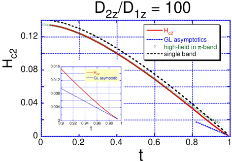
Figure 1: Temperature dependence of the upper critical field in the a-direction normalized to $H_{1}^{\parallel}$ defined in Eq. (26). Single-band curve is normalized to the corresponding scale $H_{1}$. Solid circles show the dependence obtained within the ”high-field in the $\pi$-band” approximation (Eqs. (29) and (31)). Inset: comparison between the exact solution and the GL asymptotics Eq. (42).

Numerically calculated temperature dependence of the anisotropy factor for several ratios $\mathcal{D}_{2z}/\mathcal{D}_{1z}$ is shown in Fig. 2. The anisotropy ratio drops with the increase of temperature, in accordance with the estimate (44). This result agrees qualitatively with recent measurements of temperature-dependent anisotropy in MgB₂.Sologub ; Budko ; Angst ; Eltsev ; Lyard In experiment the change in anisotropy typically is distributed over wider temperature range than it is suggested by the theory.

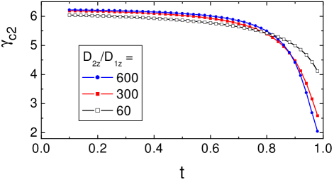
Figure 2: Temperature dependence of the anisotropy of the upper critical field for several ratios $\mathcal{D}_{2z}/\mathcal{D}_{1z}$.

V Tilted fields

The upper critical field for magnetic field tilted at angle $\theta$ with respect to $z$ axis in $(zy)$ plane is determined by the coupled linear equations for the Green’s functions $F_{\alpha}$ in two bands

$$\omega F_{\alpha}-\frac{\mathcal{D}_{\alpha x}}{2}\nabla_{x}^{2}F_{\alpha}+\frac{\mathcal{D}_{\alpha}(\theta)}{2}\left(\frac{2\pi Hx}{\Phi_{0}}\right)^{2}F_{\alpha}=\Delta_{\alpha}$$ (47)

with

$$\mathcal{D}_{\alpha}(\theta)=\mathcal{D}_{\alpha x}\cos^{2}\theta+\mathcal{D}_{\alpha z}\sin^{2}\theta$$ (48)

and the self-consistency conditions (2).

Therefore the $H_{c2}$-problem of the upper critical field in tilted field reduces to the in-plane $H_{c2}$-problem by substitution $\mathcal{D}_{\alpha z}\rightarrow\mathcal{D}_{\alpha}(\theta)$. It is convenient to introduce the angular-dependent anisotropy parameters

$$\gamma_{\alpha}(\theta)\equiv\sqrt{\frac{\mathcal{D}_{\alpha x}}{\mathcal{D}_{\alpha}(\theta)}}=\frac{\gamma_{\alpha}}{\sqrt{\gamma_{\alpha}^{2}\cos^{2}\theta+\sin^{2}\theta}}.$$ (49)

Such defined anisotropy parameters vary from $1$ to $\gamma_{\alpha}$ when angle varies from $0$ to $\pi/2$.

Following the route of the previous Section, we again use expansion with respect to the Landau levels of the strong band, defined by Eq. (17) with $\mathcal{D}_{1z}\rightarrow\mathcal{D}_{1}(\theta)$. The $F$-function of the strong band is given by

$$F_{1,n}=\frac{\Delta_{1,n}}{\omega+\varepsilon_{n}(\theta)}$$

with the eigenvalue

$$\varepsilon_{n}(\theta) =2\pi T\frac{H}{tH_{1}(\theta)}(2n+1),\$$

$$H_{1}(\theta) =\frac{2T_{c}\Phi_{0}}{\sqrt{\mathcal{D}_{1}(\theta)\mathcal{D}_{1x}}}.$$

The matrix elements for the harmonic oscillator operator of the weak band are given by

$$\epsilon_{nn} =\frac{\pi H}{\Phi_{0}}\mathcal{D}_{2}(\theta)\gamma_{1}(\theta)\left(n+\frac{1}{2}\right)\left(1+\left(\frac{\gamma_{2}(\theta)}{\gamma_{1}(\theta)}\right)^{2}\right)=\frac{2\pi T}{t_{2}(\theta)}(1+\alpha_{\gamma}(\theta))\left(n+\frac{1}{2}\right)$$

$$\epsilon_{n,n-2} =-\frac{\pi H}{\Phi_{0}}\frac{\sqrt{n(n-1)}}{2}\mathcal{D}_{2}(\theta)\gamma_{1}(\theta)\left(1-\left(\frac{\gamma_{2}(\theta)}{\gamma_{1}(\theta)}\right)^{2}\right)=-\frac{2\pi T}{t_{2}(\theta)}(1-\alpha_{\gamma}(\theta))\frac{\sqrt{n(n-1)}}{2}$$

with

$$t_{2}(\theta) =\frac{2T\Phi_{0}}{H\mathcal{D}_{2}(\theta)\gamma_{1}(\theta)}=\frac{2T\Phi_{0}\sqrt{\cos^{2}\theta+\gamma_{1}^{-2}\sin^{2}\theta}}{H\mathcal{D}_{2x}\left(\cos^{2}\theta+\gamma_{2}^{-2}\sin^{2}\theta\right)},$$

$$\alpha_{\gamma}(\theta) =\left(\frac{\gamma_{2}(\theta)}{\gamma_{1}(\theta)}\right)^{2}=\frac{1+\gamma_{1}^{-2}\tan^{2}\theta}{1+\gamma_{2}^{-2}\tan^{2}\theta}.$$

Note that at arbitrary angle we can not use inequality $\gamma_{2}(\theta)/\gamma_{1}(\theta)\ll 1$ any more. The system of equations for the reduced $F$-function at even Landau levels, $\tilde{F}_{2,n}=(2\pi T/t_{2}(\theta))F_{2,2i}$, at arbitrary tilt angle is given by

$$-(1-\alpha_{\gamma})\sqrt{i(i-1/2)}\tilde{F}_{2,i-1}+\left(z+(1+\alpha_{\gamma})\left(2i+\frac{1}{2}\right)\right)\tilde{F}_{2,i}-(1-\alpha_{\gamma})\sqrt{(i+1/2)(i+1)}\tilde{F}_{2,i+1}=\Delta_{2,2i}$$ (50)

with $z=t_{2}(\theta)(s+1/2)$.

At small tilt angles, $\theta\ll 1$, one can solve Eq. (50) using perturbation theory with respect to $\theta^{2}$. The quadratic angular correction can be obtained neglecting coupling to the higher Landau level. This leads to equation similar to Eq. (6) with replacements

$$H_{1} \rightarrow H_{1}(\theta)=\frac{2T_{c}\Phi_{0}}{\sqrt{\mathcal{D}_{1x}\mathcal{D}_{1}(\theta)}},$$

$$H_{2} \rightarrow H_{2}(\theta)=\frac{4T_{c}\Phi_{0}}{\mathcal{D}_{2}(\theta)\gamma_{1}(\theta)(1+\alpha_{\gamma})}.$$

At small angles we obtain quadratic in $\theta$ corrections to typical fields

$$H_{1}(\theta) \approx H_{1}\left(1+(1-\gamma_{1}^{-2})\frac{\theta^{2}}{2}\right),$$

$$H_{2}(\theta) \approx H_{2}\left(1+(1-\gamma_{2}^{-2})\frac{\theta^{2}}{2}\right).$$

At low temperature one can derive an exact formula for small-angle correction

$$\frac{H_{c2}(\theta)-H_{c2}(0)}{H_{c2}(0)}\approx\frac{\theta^{2}}{2}\left(1-\frac{1}{2}\left(\gamma_{1}^{-2}+\gamma_{2}^{-2}-\frac{\left(\gamma_{2}^{-2}-\gamma_{1}^{-2}\right)(W_{2}-W_{1}-\ln r_{x})}{\sqrt{\left(W_{2}+W_{1}-\ln r_{x}\right)^{2}+4W_{1}\ln r_{x}}}\right)\right)$$ (51)

with $r_{x}\equiv\mathcal{D}_{1x}/\mathcal{D}_{2x}$. In the case of small correction from the weak band, $4W_{1}\ln r_{x}\ll\left(W_{2}-\ln r_{x}\right)^{2}$, we obtain a simpler formula for $\theta\ll 1$

$$\frac{H_{c2}(\theta)-H_{c2}(0)}{H_{c2}(0)}\approx\frac{\theta^{2}}{2}\left(1-\gamma_{1}^{-2}+\frac{W_{2}W_{1}\left(\gamma_{1}^{-2}-\gamma_{2}^{-2}\right)}{\left(W_{2}-\ln r_{x}\right)^{2}}\right).$$ (52)

For parameters of MgB₂ this formula gives an estimate almost identical to the exact result.

At large tilt angles, $\cos\theta\ll 1$, inequality $\gamma_{2}(\theta)\ll\gamma_{1}(\theta)$ is restored and we can utilize the approximations used for the case of in-plane field. In particular, at low temperatures the approximate angular dependence is given by a formula similar to Eq. (35),

$$H_{c2}(\theta)\approx\frac{H_{c2}^{(1)}(0)}{\sqrt{\cos^{2}\theta+\gamma_{1}^{-2}\sin^{2}\theta}}\left(1-\frac{W_{1}\left(\ln\frac{\mathcal{D}_{2z}}{\mathcal{D}_{1x}\cot^{2}\theta+\mathcal{D}_{1z}}-1.96\right)}{W_{2}+\ln\frac{\mathcal{D}_{2z}}{\mathcal{D}_{1x}\cot^{2}\theta+\mathcal{D}_{1z}}-1.96}\right)$$ (53)

In the whole angular range we calculated the upper critical field numerically following the procedure outlined in Sec. IV.4. As input parameters we have used the values $\gamma_{1}=6.325$, $\gamma_{1}=0.816$ which follow from the electronic band-structure calculations in MgB₂. We have also used the relation $\mathcal{D}_{1x}=0.2\mathcal{D}_{2x}$ - the reason for this choice was discussed in Ref. KG, . The examples of the calculated angular dependence for $T/T_{c}=0.1$ and $0.95$ are shown in Fig. 3 . We also show fits to a simple effective-mass law, routinely used to describe angular dependence of $H_{c2}$ in anisotropic superconductors, $H_{c2}(\theta)=H_{c2,c}/\sqrt{\cos^{2}\theta+\gamma_{c2}^{-2}\sin^{2}\theta}$. Due to the contribution from the $\pi$-band, one can see significant deviations from this law at high temperature. To enhance these deviations we plot in Fig. 4 the angular dependence of the combination $\mathcal{A}(\theta)=\left(H_{c2,z}(\theta)/H_{c2,c}\right)^{2}+\left(H_{c2,x}(\theta)/H_{c2,a}\right)^{2}$ for several temperatures, (for the effective-mass law $\mathcal{A}(\theta)=1$ for all $\theta$). We find that always $\mathcal{A}(\theta)<1$ and the maximum deviation from unity is achieved around $\theta\thicksim 74^{\circ}$. At high temperatures one can derive a very simple formula for $\mathcal{A}(\theta)$ at small angles, $\theta\ll 1$, $\mathcal{A}(\theta)\approx 1-(1/\gamma_{GL}^{2}-1/\gamma_{c2}^{2})\theta^{2}$. Quantitatively, the deviations from the effective-mass law can be characterized by the parameter $\delta\mathcal{A}_{\max}=\max_{\theta}\left|1-\mathcal{A}(\theta)\right|$. Fig. 5 shows the temperature dependence of this parameter. At low temperatures deviations from the effective-mass law are at the level of several percents. These deviations progressively grow with the temperature reaching $\thicksim 19\%$ at $T/T_{c}=0.92$ and then rapidly decrease when the temperature approaches the narrow GL region near $T_{c}$. As the deviations from the effective-mass dependence have exactly the same origin as the temperature dependence of the anisotropy, it is interesting to correlate these deviations with the anisotropy change. Inset in the Fig. 5 shows plot of the parameter $\delta\mathcal{A}_{\max}$ vs the $H_{c2}$-anisotropy. One can see that the distortion of the angular dependence is maximum when the anisotropy is approximately at the midpoint between the low-temperature and GL limits. Experimentally, it was found that the angular dependence of $H_{c2}$ in MgB₂ indeed deviates from the effective mass law EltsevPhysC02 ; Welp and the shape of these deviations qualitatively agrees with our calculations.

Figure 3: Examples of angular dependence of the upper critical field at low and high temperatures. Fits to the effective-mass dependence are also shown.

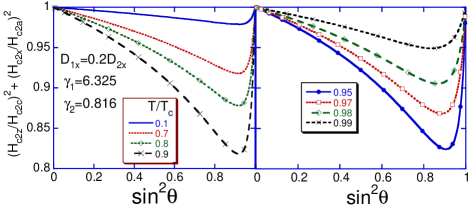
Figure 4: Plots of the parameter $\mathcal{A}(\theta)=(H_{c2,z}(\theta)/H_{c2,c})^{2}+(H_{c2,x}(\theta)/H_{c2,a})^{2}$ vs $\sin^{2}\theta$ at different temperatures revealing deviations from the simple effective-mass law. Left panel: temperatures not very close to $T_{c}$, right panel: temperature region near $T_{c}$.

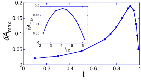
Figure 5: Temperature dependence of the parameter $\delta\mathcal{A}_{\max}=\max_{\theta}\left|1-\mathcal{A}(\theta)\right|$ characterizing deviations from the effective-mass dependence of $H_{c2}$. Inset shows the dependence of this parameter on the $H_{c2}$-anisotropy.

VI Conclusions

We have calculated the upper critical field in a dirty two-band superconductor within the quasiclassical Usadel equations, bearing in mind the regime of very high anisotropy in the quasi-2D band relevant for MgB₂. Following Ref. Mazin02, , we have assumed that the interband scattering is negligible even in the dirty limit in both bands. Most of MgB₂ samples are in dirty limit, except for single crystals, where the dirty limit conditions are fulfilled in the $\pi$-band but not fulfilled in the $\sigma$-band.YelandPRL02 Still, as argued in Ref. KG, , our results should be qualitatively applicable to MgB₂ single crystals, if one considers the coherence length $\xi_{1}$ as a phenomenological parameter instead of expressing it via the diffusion constant $\mathcal{D}_{1}$.

We have considered separately the cases when the field is parallel and perpendicular to the basal plane. We have found that at low temperatures both critical fields are mainly determined by the strong band and only weakly deviate from the universal Maki - de Gennes result. The low temperature anisotropy is mainly determined by the anisotropy of diffusion constants in a quasi-two-dimensional band. However, the anisotropy is suppressed at high temperatures. The reason is that there are two important parameters, anisotropy of pairing interaction and of diffusion constants, which enter the expression for the parallel $H_{c2}$ in a different way at high and low temperatures. This property can be expressed as the anisotropy of coherence length $\xi_{ab}/\xi_{c}$ which decreases with increasing temperature. This effect is in accordance with the experimental data in MgB₂. Note that the anisotropy of the penetration depth $\lambda_{c}/\lambda_{ab}$ increases with increasing temperature,Kogan_lam ; Golub_lam which is another manifestation of the two-band model.

We have also studied quantitatively the dependence of case of $H_{c2}$ on the angle between the ab-plane and the magnetic field direction. Approximate relations for $H_{c2}$ dependence on titled angle are derived for small and large angles. In the whole angular range numerical calculations are performed. The results demonstrate the deviation from the effective-mass dependence. This means the breakdown of anisotropic GL theory. Further, we have shown that the temperature range of applicability of the GL theory is extremely narrow in the considered two-band case.

Another issue is strong coupling corrections to $H_{c2}$. In this paper the weak coupling approach was used. On the other hand, it is known from work on isotropic superconductors SD that strong coupling corrections renormalize the absolute value of $H_{c2}$ by the factor $(1+\lambda)^{\alpha}$, where $\lambda$ is the coupling constant and $\alpha\simeq 2$. Since electron-phonon coupling in MgB₂ is relatively strong (according to Ref. Golub, , $\lambda_{11}\simeq 1$), these corrections are important for calculation of absolute values of $H_{c2}$. However, we do not expect qualitative changes in the temperature and angle dependencies of the anisotropy ratio calculated in the present paper. Extension of our results to the strong coupling Eliashberg regime is an interesting subject for future work.

We acknowledge valuable discussions with A. Brinkman, O. V. Dolgov, I. I. Mazin, U. Welp, A. Rydh, M. Iavarone, and G. Karapetrov. In Argonne this work was supported by the U.S. DOE, Office of Science, under contract # W-31-109-ENG-38.

Appendix A Local approximation for the $\pi$-band

Let us consider equation for the $F$-function in the weak $\pi$-band

$$\omega F_{2}+\frac{\mathcal{D}_{2z}}{2}\left(\frac{2\pi Hx}{\Phi_{0}}\right)^{2}F_{2}-\frac{\mathcal{D}_{2x}}{2}\nabla_{x}^{2}F_{2}=\Delta_{2}.$$ (54)

The typical scale of $\Delta_{2}(x)$ variation is imposed by the strong $\sigma$-band. This scale is given by $x_{1}=\sqrt{\gamma_{1}\Phi_{0}/2\pi H}$ and, due to inequality $\gamma_{1}\gg\gamma_{2}$, it is much larger than the length scale $x_{2}=\sqrt{\gamma_{2}\Phi_{0}/2\pi H}$ of the oscillator operator in the left side of the Eq. (54). For relevant $\omega$’s the typical length scale of $F_{2}$ variation is much larger than $x_{2}$. This allows us to neglect the gradient term in Eq. (54). This approximation is equivalent to the approximation for the matrix elements used in Eqs. (20). Then the $\pi$-band $F$-function is given by

$$F_{2}=\frac{\Delta_{2}}{\omega+\frac{\mathcal{D}_{2z}}{2}\left(\frac{2\pi Hx}{\Phi_{0}}\right)^{2}}.$$ (55)

Substituting this expression into the second self consistency equation, we represent it in the form

$$-W_{21}\Delta_{1}+W_{2}\Delta_{2}=\left(\ln\frac{1}{t}-g\left[\frac{\mathcal{D}_{2z}}{4\pi T}\left(\frac{2\pi Hx}{\Phi_{0}}\right)^{2}\right]\right)\Delta_{2}.$$ (56)

It has to be solved together with equations for $F_{1}$ and the first self consistency equation. Using expansion with respect to eigenfunctions of the $\sigma$-band $\Psi_{n}(x)$, this equation reduces to the form of linear equation (25b), in which the matrix $U_{i,j}$ is given by the matrix elements

$$U_{i,j}=-\int dx\Psi_{2i}(x)\Psi_{2j}(x)g\left[\frac{\mathcal{D}_{2z}}{4\pi T}\left(\frac{2\pi Hx}{\Phi_{0}}\right)^{2}\right].$$

Introducing the dimensionless oscillator wave functions $\psi_{n}(\tilde{x})$, $\Psi_{n}(x)=\psi_{n}(x/x_{1})/\sqrt{x_{1}}$, we present these matrix elements in the dimensionless form

$$U_{i,j}(t_{2})=\int_{-\infty}^{\infty}d\tilde{x}\psi_{2i}(\tilde{x})\psi_{2j}(\tilde{x})g\left[\tilde{x}^{2}/t_{2}\right],$$

where, again $1/t_{2}\equiv\left(\mathcal{D}_{2z}/\mathcal{D}_{1z}\right)\left(H/tH_{1}\right)$. In particular, $\psi_{0}(\tilde{x})=\pi^{-1/4}\exp(-\tilde{x}^{2}/2)$. In the ”high-field in $\pi$-band” regime, $t_{2}\ll 1$, one can use asymptotics $g\left[\tilde{x}^{2}/t_{2}\right]\approx 2\ln(\tilde{x})-\ln t_{2}+\gamma_{E}+2\ln 2$ and obtain

$$U_{i,j}(t_{2}) =f_{i,j}+(\ln t_{2}-\gamma_{E}-2\ln 2)\delta_{n,m}$$

$$f_{i,j} =-4\int_{0}^{\infty}d\tilde{x}\psi_{2i}(\tilde{x})\psi_{2j}(\tilde{x})\ln(\tilde{x}).$$

In particular,

$$f_{0,0}=-\frac{4}{\sqrt{\pi}}\int d\tilde{x}\exp(-\tilde{x}^{2})\ln(\tilde{x})=\gamma_{E}+2\ln 2\approx 1.9635$$

References

- (1) J. Nagamatsu, N. Nakagawa, T. Muranaka, Y. Zenitani, and J. Akimitsu, Nature 410, 63 (2001).
- (2) H. Suhl, B.T. Matthias, and L.R. Walker, Phys. Rev. Lett. 3, 552 (1959).
- (3) V.A. Moskalenko, Fiz. Met. Met. 4, 503 (1959).
- (4) J. Kortus, I.I. Mazin, K.D. Belashchenko, V.P. Antropov, L.L. Boyer, Phys. Rev. Lett. 86, 4656 (2001).
- (5) J. N. An and W. E. Pickett, Phys. Rev. Lett. 86, 4366 (2001).
- (6) A. Y. Liu, I. I. Mazin, and J. Kortus, Phys. Rev. Lett. 87, 087005 (2001).
- (7) S. V. Shulga, S.- L. Drechsler, H. Eschrig, H. Rosner, and W. E. Pickett, eprint cond-mat/0103154.
- (8) Y. Kong, O. V. Dolgov, O. Jepsen, and O. K. Andersen , Phys. Rev. B 64, 020501(R) (2001).
- (9) T. Yildirim, O. Gülseren, J. W. Lynn, C. M. Brown, T. J. Udovic, Q. Huang, N. Rogado, K. A. Regan, M. A. Hayward, J. S. Slusky, T. He, M. K. Haas, P. Khalifah, K. Inumaru, and R. J. Cava , Phys. Rev. Lett. 87, 037001 (2001).
- (10) H. J. Choi, D. Roundy, H. Sun, M. L. Cohen, and G. Louie, Phys. Rev. B, 66, 020513 (2002); Nature 418, 758 (2002).
- (11) A. A. Golubov, J. Kortus, O. V. Dolgov, O. Jepsen, Y. Kong, O. K. Andersen, B. J. Gibson, K. Ahn, and R. K. Kremer, J.Phys.: Condens. Matter, 14, 1353 (2002).
- (12) A. Brinkman, A. A. Golubov, H. Rogalla, O. V. Dolgov, J. Kortus, Y. Kong, O. Jepsen, O. K. Andersen, Phys. Rev. B, 65, 180517 (2002).
- (13) I. I. Mazin, O. K. Andersen, O. Jepsen, O. V. Dolgov, J. Kortus, A. A. Golubov, A. B. Kuz’menko, and D. van der Marel, Phys. Rev. Lett. 89 107002 (2002).
- (14) F. Giubileo, D. Roditchev, W. Sacks, R. Lamy, D.X.Thanh, J. Klein, S. Miraglia, D. Fruchart, J. Marcus, and Ph. Monod, Phys. Rev. Lett. 87, 177008 (2001).
- (15) M. Iavarone, G. Karapetrov, A. E. Koshelev, W. K. Kwok, G. W. Crabtree, D. G. Hinks, W. N. Kang, Eun-Mi Choi, Hyun Jung Kim, Hyeong-Jin Kim, and S. I. Lee Phys. Rev. Lett. 89, 187002 (2002).
- (16) P. Szabó, P. Samuely, J. Kacmarcik, T. Klein, J. Marcus, D. Fruchart, S. Miraglia, C. Mercenat, and A. G. M. Jansen, Phys. Rev. Lett. 87, 137005 (2001).
- (17) H. Schmidt, J. F. Zasadzinski, K. E. Gray, and D. G. Hinks, Phys. Rev. Lett. 88, 127002 (2001).
- (18) R. S. Gonnelli, D. Daghero, G. A. Ummarino, V. A. Stepanov, J. Jun, S. M. Kazakov, and J. Karpinski, Phys. Rev. Lett. 89, (2002).
- (19) F. Bouquet, R. A. Fisher, N. E. Phillips, and D. G. Hinks, and J. D. Jorgensen, Phys. Rev. Lett. 87, 047001 (2001).
- (20) M. R. Eskildsen, M. Kugler, S. Tanaka, J. Jun, S. M. Kazakov, J. Karpinski, and Ø. Fischer, Phys. Rev. Lett. 89, 187003 (2002).
- (21) A. E. Koshelev and A. A. Golubov, eprint cond-mat/0211288.
- (22) A. Nakai, M. Ichioka, and K. Machida, J. Phys. Soc. Jap. 71, 23 (2002).
- (23) V. Kogan and S. L. Budko, Physica C 385, 131 (2003).
- (24) V. Kogan, Phys. Rev. B 66, R020609 (2002).
- (25) A. A. Golubov, A. Brinkman, O. V. Dolgov, J. Kortus, and O. Jepsen, Phys. Rev. B 66, 054524 (2002).
- (26) P. Miranović, K. Machida, and V. G. Kogan, eprint cond-mat/0207146.
- (27) T. Dahm and N. Schopohl, eprint cond-mat/0212188.
- (28) A. V. Sologubenko, J. Jun, S. M. Kazakov, J. Karpinski, and H. R. Ott, Phys. Rev. B 65, 180505(R) (2002).
- (29) S. L. Bud’ko and P. C. Canfield, Phys. Rev. B 65, 212501 (2002).
- (30) M. Angst, R. Puzniak, A. Wisniewski, J. Jun, S. M. Kazakov, J. Karpinski, J. Roos, and H. Keller, Phys. Rev. Lett. 88, 167004 (2002).
- (31) Yu. Eltsev, S. Lee, K. Nakao, N. Chikumoto, S. Tajima, N. Koshizuka, and M. Murakami, Phys. Rev. B 65, 140501(R) (2002); Physica C 378-381, 61 (2002).
- (32) L. Lyard, P. Samuely, P. Szabo, T. Klein, C. Marcenat, L. Paulius, K. H. P. Kim, C. U. Jung, H.-S. Lee, B. Kang, S. Choi, S.-I. Lee, J. Marcus, S. Blanchard, A.G.M. Jansen, U. Welp, G. Karapetrov, W.K. Kwok, Phys. Rev. B 66, 180502(R) (2002).
- (33) U. Welp, A. Rydh, G. Karapetrov, W. K. Kwok, G. W. Crabtree, Ch. Marcenat, L. Paulius, T. Klein, J. Marcus, K. H. P. Kim, C. U. Jung, H.-S. Lee, B. Kang, and S.-I. Lee, Phys. Rev. B 67, 012505 (2003).
- (34) K. Usadel, Phys. Rev. Lett. 25, 507 (1970); Phys. Rev. B 4, 99 (1971).
- (35) A. Gurevich, eprint cond-mat/0212129.
- (36) The parameter is related with the parameter from Ref. Dahm, as .
- (37) This limit corresponds to Eq. (35) of Ref. Gurevich, . However this formula is written with a typo: there should be a minus sign in front of inside the exponential factor.
- (38) K. Maki, Physics, 1, 21 (1964).
- (39) P. G. de Gennes, Phys. Kondensierten Materie, 3, 79 (1964).
- (40) E. Langmann, Phys. Rev. B 46, 9104 (1992).
- (41) E. A. Yelland, J. R. Cooper, A. Carrington, N. E. Hussey, P. J. Meeson, S. Lee, A. Yamamoto, and S. Tajima, Phys. Rev. Lett. 88, 217002 (2002).
- (42) S.V. Shulga and S.-L. Drechsler, eprint cond-mat/0202172.
- (43) Yu. Eltsev, S. Lee, K. Nakao, N. Chikumoto, S. Tajima, N. Koshizuka and M. Murakami, Physica C, 378-381, 61 (2002).
- (44) U. Welp et. al. to be published