Infinite family of persistence exponents for interface fluctuations

Abstract

We show experimentally and theoretically that the persistence of large deviations in equilibrium step fluctuations is characterized by an infinite family of independent exponents. These exponents are obtained by carefully analyzing dynamical experimental images of Al/Si(111) and Ag(111) equilibrium steps fluctuating at high (970K) and low (320K) temperatures respectively, and by quantitatively interpreting our observations on the basis of the corresponding coarse-grained discrete and continuum theoretical models for thermal surface step fluctuations under attachment/detachment (“high-temperature”) and edge-diffusion limited kinetics (“low-temperature”) respectively.

Persistence is a fundamental and powerful concept in the stochastic dynamics of non-Markovian statistical processes 1 . Recently, the persistence concept has been applied to statistical studies of spatially extended non-equilibrium systems both theoretically 3 and experimentally 4 . Loosely speaking, persistence is the probability $P(t)$ that a stochastic variable, which is found to have a “positive” value at time $t_{0}$, will stay “positive” throughout a time interval $t$ up to time $t_{0}+t$. In most steady-state (“stationary”) situations, the persistence probability is found to decay in time in a power-law manner, $P(t)\sim t^{-\theta}$, for large $t$, where the persistence exponent $\theta$ is a highly nontrivial exponent characterizing the relevant stochastic dynamics under consideration. The concept of persistence has been used 6 ; 7 ; 8 to study the interesting problem of thermally fluctuating interfaces where steps on vicinal surfaces undergo random thermal motion in equilibrium 5 . The step persistence probability is the probability $P(t_{0},t_{0}+t)$ that a given lateral step position $x$ with a height (i.e. step fluctuation measured from the equilibrium step position) $h(x,t_{0})$ at time $t_{0}$ does not return to this value up to a later time $t_{0}+t$. With no loss of generality we will set $t_{0}=0$ from now on, assuming that thermal equilibrium has been achieved in the step fluctuations and we are discussing steady-state stationary properties. The resulting persistence probability $P(t)\equiv P(0,t)$ has recently been studied experimentally using dynamical scanning tunneling microscopy (STM) in two systems: Al steps on Si $(111)$ surface at high temperatures $\sim 970$K 7 and Ag $(111)$ surface at low temperatures $\sim 320$K 8 . In the first case, the step fluctuations dominated by atomistic attachment and detachment (AD) at the step edge are known 5 to be well described by the coarse-grained second-order non-conserved linear Langevin equation

$$\frac{\partial h(x,t)}{\partial t}=\frac{\partial^{2}h(x,t)}{\partial x^{2}}+\eta(x,t),$$ (1)

where $\eta(x,t)$ with $\langle\eta(x,t)\eta(x^{{}^{\prime}},t^{{}^{\prime}})\rangle\propto\delta(x-x^{{}^{\prime}})\delta(t-t^{{}^{\prime}})$ is the usual uncorrelated random Gaussian noise corresponding to the non-conserved white noise associated with the random AD process. Low temperature step fluctuations dominated by the step edge diffusion (ED) mechanism are, on the other hand, described by a fourth order conserved linear Langevin equation:

$$\frac{\partial h(x,t)}{\partial t}=-\frac{\partial^{4}h(x,t)}{\partial x^{4}}+\eta_{c}(x,t),$$ (2)

where $\eta_{c}(x,t)$ with $\langle\eta_{c}(x,t)\eta_{c}(x^{{}^{\prime}},t^{{}^{\prime}})\rangle\propto\nabla^{2}\delta(x-x^{{}^{\prime}})\delta(t-t^{{}^{\prime}})$ is a conserved noise associated with atomic diffusion along the step edge. From a quantitative analysis of the digitized STM step images as a function of time, the persistence exponent was found to be $\theta=0.77\pm 0.03$ 7 and $\theta=0.87\pm 0.02$ 8 , respectively, for the high-temperature AD mechanism and low-temperature ED mechanism. These measured step fluctuation persistence exponents agree reasonably well with those found 6 from kinetic Monte Carlo simulations of the corresponding discrete solid-on-solid models: $\theta\simeq 0.75$ (for Eq. (1)) and $\theta\simeq 0.86$ (for Eq. (2)). These results are in agreement with a postulated (and numerically verified) relation 6 between persistence in the steady state and dynamic scaling 9 in the pre-stationary transient regime. It is believed 6 that, at least for linear Langevin equations, the persistence exponent $\theta$ is equal to $(1-\beta)$ where $\beta$ is the exponent that describes the initial power-law growth of the interface width 9 in the transient regime ($\beta=1/4$ for Eq. (1) and $\beta=1/8$ for Eq. (2)).

This striking agreement between experimentally obtained and theoretically predicted values of the persistence exponent demonstrates the overall excellent consistency among theory, experiment, and simulations in this problem, but also brings up a key question regarding persistence studies 6 ; 7 ; 8 of surface fluctuations: Is persistence really an independent (and new) conceptual tool in studying surface fluctuations, or, is it just an equivalent (perhaps even complementary) way of studying dynamic scaling 5 ; 9 of height correlations? In this Letter we present new theoretical and experimental persistence results on surface step fluctuations that fundamentally transcend any dynamic scaling considerations, establishing in the process the existence of a novel and nontrivial infinite family (i.e. a continuous set) of persistence exponents for equilibrium step fluctuations. We carry out quantitative analyses of (digitized) dynamical STM images of step fluctuations both for high-temperature (Al/Si) and low-temperature (Ag) equilibrium surfaces, and compare in details the experimental results with those we have obtained from numerical integration of the corresponding Langevin equations and discrete stochastic Monte Carlo simulations of corresponding atomistic cellular automata type models in the same dynamical universality classes 5 ; 9 . All three sets of persistence results agree very well for both high and low temperature equilibrium step fluctuations, establishing persistence (particularly, the infinite family of persistence exponents) as a potentially powerful tool (rivaling, perhaps even exceeding, in utility the well-studied dynamic scaling approach) in studying dynamical interface fluctuation processes.

The infinite family of persistence exponents we study here is based on the concept of persistence of large deviations introduced recently by Dornic and Godreche 10 in the context of kinetic Glauber-Ising dynamics of magnetization coarsening (a closely related idea, that of sign-time distribution, was developed in Ref. 12 ). For equilibrium step fluctuations, we define the probability of persistent large deviations, $P(t,s)$, as the probability for the “average sign” $S_{\text{av}}$ of the height fluctuation to remain above a certain pre-assigned value “$s$” up to time $t$:

$$P(t,s)\equiv\hbox{Prob}~{}\{~{}S_{\text{av}}(t^{\prime})\geq s,~{}\forall t^{\prime}\leq t~{}\},$$ (3)

where

$$S_{\text{av}}(t)\equiv t^{-1}\int_{0}^{t}{dt^{\prime}~{}S(t^{\prime})},$$ (4)

and

$$S(t)\equiv\hbox{sign}~{}[h(x,t_{0}+t)-h(x,t_{0})],$$ (5)

where with no loss of generality, we set $t_{0}=0$. Although the dynamical variable $S(t)$ above is defined for a particular lateral position $x$, we take a statistical ensemble average over all lateral positions to obtain a purely time dependent dynamical quantity $P(t,s)$. Since $S_{\text{av}}(t)\in[-1,1]$, the probability $P(t,s)$ is defined for $-1\leq s\leq 1$. For $s=1$ we recover our earlier simple definition of persistence used in Refs. 6 ; 7 ; 8 : $P(t)\equiv P(t,s=1)$ measures the probability of the height fluctuation remaining above zero (“positive”) throughout the whole time interval. For $s=-1$ the probability $P(t,s=-1)$ is trivially equal to unity for all $t$. The generalized probability function, $P(t,s)$, defined in Eqs. (3)–(5) above, leads to a continuous family or hierarchy of persistent large deviations exponents, $\theta_{l}(s)$, provided the steady-state decay of $P(t,s)$ in time follows a power law, $P(t,s)\sim t^{-\theta_{l}(s)}$. As we show below, this indeed happens for equilibrium step fluctuation phenomena, allowing us to define and measure the non-trivial persistence exponent $\theta_{l}(s),\,-1\leq s\leq 1$, that varies continuously between $\theta_{l}(s=-1)\equiv 0$ and $\theta_{l}(s=+1)\equiv\theta$ where $\theta$ is the usual persistence exponent. Clearly, $P(t,s)$ and $\theta_{l}(s)$ are natural generalizations of the persistence probability $P(t)$ and the persistence exponent $\theta$, respectively, to the broader concept of distribution of residence times with limiting behavior (i.e. $s=1$) determining the usual persistence exponent.

In this Letter, we have carried out the first application of the persistent large deviations concept to the equilibrium step fluctuations phenomenon. We also report the first experimental measurements of $P(t,s)$ and $\theta_{l}$ for any stochastic system. Our results for the two distinct types of step fluctuation processes (the high-temperature AD and low-temperature ED situations, described 5 by Eqs. (1) and (2), respectively) are shown in Figs. 1 and 2. The details of the experimental procedure for extracting the persistence probability from the digitized dynamical STM images are described in Refs. 7 ; 8 for the same two systems, and are therefore not repeated here. We only mention that in order to obtain the probability of persistent large deviations, we had to use a substantially larger number ($\sim 100$) of STM data sets than that used in Refs. 7 ; 8 . As mentioned earlier, we compare the experimental results with two theoretical models in each case: The continuous Langevin equation (Eq. (1) or (2)) and a discrete stochastic model which is theoretically known 6 ; 7 ; 8 ; 5 ; 9 to belong to the same universality class (in the dynamic scaling sense) as the continuum equation. For the high-temperature AD step fluctuations, described on a coarse-grained scale by Eq. (1) (sometimes referred to as the Edwards–Wilkinson equation 9 ), the discrete stochastic model we use is the extensively studied solid-on-solid Family model 9 ; 13 . For the low-temperature ED case, described on a coarse-grained scale by Eq. (2) (sometimes referred to as the Mullins–Herring equation with conserved noise 9 ), the discrete stochastic model we use is the well-studied Racz model 14 . Our results are obtained from numerical integration of the Langevin equations using the simple Euler scheme 6 , and standard Monte Carlo simulation 6 of the atomistic models. Typical system sizes used in the numerical work are $\sim 1000$ for Eq.(1) and $\sim 100$ for Eq.(2), and the number of independent runs used in the calculation of persistence probabilities is $\sim 1000$.

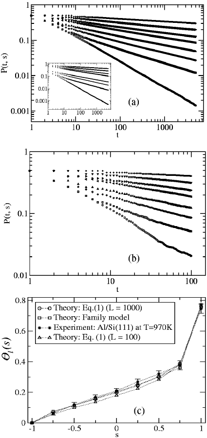
Figure 1: Log-log plots of the persistent large deviations probability, $P(t,s)$, for high-temperature surface step fluctuations via the AD mechanism, shown as a function of time ($t$) for different values of the average sign constraint parameter $s=1.0,~{}0.75,~{}0.5,~{}0.25,~{}0,-0.25,-0.5,-0.75$ (from the bottom to the top). (a) The continuum Langevin equation of Eq.(1) (main figure) and the stochastic discrete Family model (inset); (b) experimental data from digitized dynamical STM step images of Al on Si(111) surface; and (c) comparison of the various sets of results for $\theta_{l}$ as a function of $s$. The error bars shown for the experimental data are obtained from variations of the local slope of the $\log P(t,s)$ vs $\log t$ plots. Simulation results for two sample sizes ($L=100$ and $L=1000$) are shown to illustrate that the use of small samples leads to an underestimation of $\theta_{l}(s)$.

In Fig. 1 we show in the top two panels our measured (panel (b)) and calculated (panel (a), main figure and inset) persistent large deviation probability $P(t,s)$ as a function of time $t$ for the high-temperature step fluctuations case. Each panel shows eight different log-log plots of $P(t,s)$ against $t$ for eight different values of the average sign parameter $s~{}(=+1,+0.75,...,-0.75$ from the bottom to the top). As mentioned before, the case $s=+1$ (the bottom-most curve) corresponds to the usual persistence probability $P(t)$, and therefore the results shown in Fig. 1 for $s=1$ are already known. The results for all the other values of $s$ are new and non-trivial. The linearity of the log-log $P(t,s)$ vs. $t$ plots immediately implies that $P(t,s)\sim t^{-\theta_{l}(s)}$. The different sets of results for $\theta_{l}$ as a function of $s$ are shown in Fig. 1(c). The excellent agreement among the various data sets shown in Fig. 1(c) is the most important new quantitative result of our work. This means that the high-temperature step fluctuation phenomenon via the AD mechanism is indeed described by the Edwards–Wilkinson equation (and therefore also by the discrete Family model), not just in the sense of the dynamical universality class (as defined by specific exponent values, e.g. $\beta$ and $\theta$) but more importantly for the infinite family of persistent large deviations exponents as defined by the continuous function $\theta_{l}(s)$. This striking agreement between experiment and theory for a continuous family of exponents definitely establishes persistent large deviations studies as a new and effective tool for studying dynamical fluctuations of nanoscale systems.

Figure 2: The same as in Fig. 1 for the low-temperature step fluctuations via the ED mechanism. (a) The continuum Langevin equation of Eq. (2) (main figure) and the discrete stochastic Racz model (inset); (b) experimental data for the Ag(111) step fluctuations; and (c) comparison of the three sets of results for $\theta_{l}$: experiment (star), stochastic Racz model (square) and Eq. (2) (circle). The inset shows the time-dependence of the local exponent $\theta_{l}(s,t)$ obtained from simulations of the Langevin equation for $s=0.25$ and $s=0.50$.

In Fig. 2 we present results similar to those in Fig. 1, but now for the ED mechanism step fluctuation data along with the corresponding theoretical results for the continuum Langevin equation defined by Eq. (2) and the discrete stochastic Racz model which are known 6 ; 8 ; 5 ; 13 to be in the same dynamic universality class as the low-temperature step fluctuation process. The same description and explanation given above for Fig. 1 apply now to Fig. 2 where $\theta_{l}(s=1)\approx 0.875$, which agrees with recent experimental measurements 8 of the usual persistence exponent of low-temperature step fluctuations on Ag and Pb surfaces. The experimental and theoretical results for the continuous function $\theta_{l}(s)$, shown in Fig. 2(c), exhibit qualitative agreement, with the experimental exponent values for $s<1$ being slightly larger than the theoretical ones. There are several possible explanations for this difference between experimental and theoretical results. There are reasons to expect that increasing the dynamic range of the experimental $P(t,s)$ beyond two decades in $t$ (this range is limited by noise problems inherent in dynamic STM imaging) would bring theory and experiment into closer agreement. To illustrate this possibility, we show in the inset of Fig. 2(c) the time-dependence of the local exponent $\theta_{l}(s,t)=d\log[P(s,t)]/d\log t$, obtained from simulations of the Langevin equation for two values of $s$ for which the difference between theory and experiment is large. The local exponent is found to decrease with time before reaching a constant value at large $t$. We have checked that the experimental data show similar behavior for all $s<1$, which implies that the effective exponent values obtained from power-law fits of relatively short-time data would be larger than the true long-time values. Indeed, we have found that fits of the simulation data over the range $20\leq t\leq 200$ (this is the range used in obtaining $\theta_{l}(s)$ from the experimental data) yield values of $\theta_{l}(s)$ that are higher and closer to the experimental values. A second possibility is that the smallness of the sample size used in the simulations leads to an underestimation of the values of $\theta_{l}(s)$, as in Fig. 1(c). Unfortunately, the impossibility of equilibrating much larger samples of these models with very slow dynamics prevents us from checking this explicitly. Another possibility that we can not rule out is that the Ag(111) equilibrium step fluctuations do not precisely follow the theoretical models of edge-diffusion limited kinetics. Further experimental and theoretical investigations would be needed for settling this issue. We should emphasize, however, that given the severe complexity in measuring any power law exponents associated with surface step fluctuation dynamics, the overall agreement between theory and experiment is quite good.

In summary, we have established the concept (and the usefulness) of an infinite family of persistent large deviations exponents for height fluctuations in equilibrium surface step dynamics phenomenon. The impressive agreement between theory and experiment indicates that the persistent large deviations probability (and the corresponding exponents) may very well be an extremely powerful tool in characterizing and understanding other stochastic fluctuation phenomena, e.g., kinetic surface roughening in nonequilibrium growth. In contrast to other dynamical approaches, the technique developed in this Letter leads to a continuous family of exponents (a continuous function rather than one or two isolated independent exponents (as in the dynamic scaling approach) and is therefore a much more stringent test of theoretical ideas, and also perhaps provides a deeper level of probing the dynamics of fluctuation problems.

This work is partially supported by the NSF-DMR-MRSEC at the University of Maryland.

References

- (1) S. N. Majumdar, Curr. Sci. 77, 370 (1999).
- (2) B. Derrida et al., J. Phys. A 27, L357 (1994); S. N. Majumdar et al., Phys. Rev. Lett. 77, 2867 (1996); B. Derrida et al., Phys. Rev. Lett. 77, 2871 (1996).
- (3) M. Marcos-Martin et al., Physica A 214, 396 (1995); B. Yurke et al., Phys. Rev. E 56, R40 (1997); W. Y. Tam et al., Phys. Rev. Lett. 78, 1588 1997); G. P. Wong et al., Phys. Rev. Lett 86, 4156 (2001).
- (4) J. Krug et al.Phys. Rev. E 56, 2702 (1997).
- (5) D. B. Dougherty et al., Phys. Rev. Lett 89, 136102 (2002).
- (6) D. B. Dougherty et al., Surf. Sci. 527 L213 (2003).
- (7) H. Jeong and E. D. Williams, Surf. Sci. Reports 34, 171 (1999); I. L. Lyubinetsky et al., Phys. Rev. B 66, 085327 (2002)
- (8) A. -L. Barabasi and H. E. Stanley, Fractal Concepts in Surface Growth (Cambridge, New York, 1995).
- (9) I. Dornic and C. Godreche, J. Phys. A: Math. Gen. 31, 5413 (1998).
- (10) Z. Toroczkai et al., Phys. Rev. E 60, R1115 (1999).
- (11) F. Family, J. Phys. A: Gen. 19, L441 (1986).
- (12) Z. Racz et al., Phys. Rev. A 43, 5275 (1991).