Feshbach resonances and collapsing Bose-Einstein condensates

Abstract

We investigate the quantum state of burst atoms seen in the recent Rb-85 experiments at JILA. We show that the presence of a resonance scattering state can lead to a pairing instability generating an outflow of atoms with energy comparable to that observed. A resonance effective field theory is used to study this dynamical process in an inhomogeneous system with spherical symmetry.

1 Introduction

The ability to dynamically modify the nature of the microscopic interactions in a Bose-Einstein condensate—an ability virtually unique to the field of dilute gases—opens the way to the exploration of a range of fundamental phenomena. A striking example of this is the Bosenova experiment carried out in the Wieman group at JILA [1] which explored the mechanical collapse instability arising from an attractive interaction. This collapse resulted in an unanticipated burst of atoms, the nature of which is a subject of current debate. In this article we suggest a possible mechanism for the formation of these bursts by application of an effective quantum field theory which includes explicitly the resonance scattering physics.

The Bosenova experiment conducted by the JILA group consisted of the following elements. A conventional stable Bose-Einstein condensate was created in equilibrium. The group then utilized a Feshbach resonance to abruptly switch the interactions to be attractive inducing an implosion. One might have predicted that the rapid increase in density would simply lead to a rapid loss of atoms, primarily through inelastic three-body collisions. In contrast, what was observed was the formation of an energetic burst of atoms emerging from the implosion. Although the energy of these atoms was much larger than that of the condensate, the energy was insignificant when compared to the molecular binding energy which characterizes the energy released in a three-body collision. In the end, what remained was a remnant condensate which appeared distorted and was believed to be in a highly excited collective state.

One theoretical method which has been extensively explored to explain this behavior has been the inclusion of a decay term into the Gross-Pitaevskii equation as a way to account for the atom loss [2, 3, 4, 5]. Aside from its physical application to the Bosenova problem, the inclusion of three-body loss as a phenomenological mechanism represents an important mathematical problem, since the nonlinear Schrödinger equation allows for a class of self-similar solutions in the unstable regime. The local collapses predicted in this framework can generate an outflow even within this zero temperature theory. However, there are a number of aspects which one should consider when applying the extended Gross-Pitaevskii equation to account for the observations made in the JILA experiment.

The first problematic issue is the potential breakdown of the principle of attenuation of correlations. This principle is essential in any quantum or classical kinetic theory as it allows multiparticle correlations to be factorized. This assumption is especially evident in the derivation of the Gross-Pitaevskii equation where all explicit multiparticle correlations are dropped. However, as shown in Figure 1, even a simple classical model may exhibit clustering when mechanically unstable which appears to invalidate the assumption of an attenuation of correlations. Furthermore, there is also considerable evidence for this instability toward pair formation in the mechanically unstable quantum theory [6].

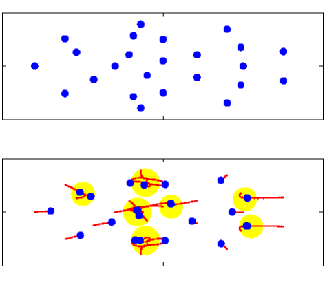
Figure 1: A collapsing classical system with point-like objects interacting via a Gaussian attractive potential. The top graph shows the initial configuration. The lower graph displays the evolved state demonstrating clustering of the particles (illustrated as yellow regions). The red lines mark the particle trajectories.

A second difficulty with motivating the Gross-Pitaevskii approach is that by this method one describes the interactions as energy independent through a single parameter, the scattering length, which is determined from the $s$-wave scattering phase shift at zero scattering energy. Near a Feshbach resonance, the proximity of a bound state in a closed potential to the zero of the scattering continuum can lead to a strong energy dependence of the scattering. Exactly on resonance, the $s$-wave scattering length passes through infinity and, in this situation, the Gross-Pitaevskii equation is undefined.

These two fundamental difficulties with the Gross-Pitaevskii approach led us to reconsider this problem. We were motivated by the fact that the same experimental group at JILA recently performed a complementary experiment [7] which provided key insights into the Bosenova system. What was remarkable in these new experiments was that, even with a large positive scattering length in which the interactions were repulsive, a burst of atoms and a remnant condensate were observed. Furthermore, in the large positive scattering length case, simple effective field theories which included an explicit description of the Feshbach resonance physics were able to provide an accurate quantitative comparison with the data [8, 9, 10]. The theory showed the burst to arise from the complex dynamics of the atom condensate coupled to a coherent field of exotic molecular dimers of a remarkable physical size and near the threshold binding energy.

In this paper, we draw the connections between the two JILA experiments. We pose and resolve the question as to whether the burst of atoms in the Bosenova collapse could arise in a similar way as in the Ramsey fringe experiment—from the formation of a coherent molecular superfluid. This hypothesis is tested by applying an effective field theory for resonance superfluidity to the collapse. For fermions, the case of resonance superfluidity in an inhomogeneous system has been treated in the local density approximation, using essentially the uniform solution at each point in space [11]. For the collapse of a Bose-Einstein condensate, as we wish to treat here, the local density approximation is not valid, and the calculation must be performed on a truly inhomogeneous system. This represents the first time that the resonance superfluidity theory has been applied to a system of this type.

2 Effective Field Theory

In the Feshbach resonance illustrated in Figure 2, the properties of the collision of two ground state atoms is controlled through their resonant coupling to a bound state in a closed channel Born-Oppenheimer potential. By adjusting an external magnetic field, the scattering length can be tuned to have any value. This field dependence of the scattering length is characterized by the detuning $\nu_{0}$ and obeys a dispersive profile given by $a(\nu_{0})=a_{\rm bg}(1-\kappa/(2\nu_{0}))$, with $\kappa$ the resonance width and $a_{\rm bg}$ the background scattering length. In fact, all the scattering properties of a Feshbach resonance system are completely characterized by just three parameters $U_{0}=4\pi\hbar^{2}a_{\rm bg}/m$, $g_{0}=\sqrt{\kappa U_{0}}$, and $\nu_{0}$. Physically, $U_{0}$ represents the energy shift per unit density on the single particle eigenvalues due to the background scattering processes, while $g_{0}$, which has dimensions of energy per square-root density, represents the coupling of the Feshbach resonance between the open and closed channel potentials.

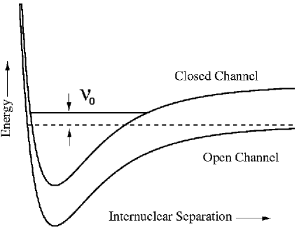
Figure 2: A Feshbach resonance results when a closed channel potential possesses a bound state in proximity to the scattering energy in an open channel potential. The detuning of the bound state from the edge of the collision continuum is denoted by $\nu_{0}$.

We now proceed to construct a low order many-body theory which includes this resonance physics. The Hamiltonian for a dilute gas of scalar bosons with binary interactions is given in complete generality by

$$H=\int d^{3}x\;\psi^{{\dagger}}_{a}({\mbox{\boldmath$x$}})H_{a}({\mbox{\boldmath$x$}})\psi_{a}({\mbox{\boldmath$x$}})+\int d^{3}xd^{3}x^{\prime}\;\psi^{{\dagger}}_{a}({\mbox{\boldmath$x$}})\psi^{{\dagger}}_{a}({\mbox{\boldmath$x^{\prime}$}})V({\mbox{\boldmath$x$}},{\mbox{\boldmath$x^{\prime}$}})\psi_{a}({\mbox{\boldmath$x^{\prime}$}})\psi_{a}({\mbox{\boldmath$x$}})$$ (1)

where $H_{a}({\mbox{\boldmath$x$}})$ is the single particle Hamiltonian, $V({\mbox{\boldmath$x$}},{\mbox{\boldmath$x^{\prime}$}})$ is the binary interaction potential, and $\psi_{a}({\mbox{\boldmath$x$}})$ is a bosonic scalar field operator. In cold quantum gases, where the atoms collide at very low energy, we are only interested in the behavior of the scattering about a small energy range above zero. There exist many potentials which replicate the low energy scattering behavior of the true potential; therefore, it is convenient to carry out the calculation with the simplest one, the most convenient choice being to take the interaction potential as a delta-function pseudopotential when possible.

For a Feshbach resonance this choice of pseudopotential is generally not available since the energy dependence of the scattering implies that a minimal treatment must at least contain a spread of wave-numbers which is equivalent to the requirement of a nonlocal potential. Since the solution of a nonlocal field theory is inconvenient, we take an alternative but equivalent approach. We include into the theory an auxiliary molecular field operator $\psi_{m}({\mbox{\boldmath$x$}})$ which obeys Bose statistics and describes the collision between atoms in terms of two elementary components: the background collisions between atoms in the absence of the resonance interactions and the conversion of atom pairs into molecular states. This allows us to construct a local field theory with the property that when the auxiliary field is integrated out, an effective Hamiltonian of the form given in Eq. (1) is recovered with a potential $V({\mbox{\boldmath$x$}},{\mbox{\boldmath$x$}}^{\prime})=V(|{\mbox{\boldmath$x$}}-{\mbox{\boldmath$x$}}^{\prime}|)$ which generates the form of the two-body $T$-matrix predicted by Feshbach resonance theory [12]. The local Hamiltonian which generates this scattering behavior:

$$H = \int d^{3}x\;\psi^{{\dagger}}_{a}({\mbox{\boldmath$x$}})\Bigl{(}-\frac{\hbar^{2}}{2m}\nabla_{x}^{2}+V_{a}({\mbox{\boldmath$x$}})-\mu_{a}\Bigr{)}\psi_{a}({\mbox{\boldmath$x$}})$$ (2)

$$+\int d^{3}x\;\psi^{{\dagger}}_{m}({\mbox{\boldmath$x$}})\Bigl{(}-\frac{\hbar^{2}}{4m}\nabla_{x}^{2}+V_{m}({\mbox{\boldmath$x$}})-\mu_{m}\Bigr{)}\psi_{m}({\mbox{\boldmath$x$}})$$

$${}+{U\over 2}\int d^{3}x\;\psi^{{\dagger}}_{a}({\mbox{\boldmath$x$}})\psi^{{\dagger}}_{a}({\mbox{\boldmath$x$}})\psi_{a}({\mbox{\boldmath$x$}})\psi_{a}({\mbox{\boldmath$x$}})$$

$${}+{g\over 2}\int d^{3}x\;\psi^{{\dagger}}_{m}({\mbox{\boldmath$x$}})\psi_{a}({\mbox{\boldmath$x$}})\psi_{a}({\mbox{\boldmath$x$}})$$

has the intuitive structure of resonant atom-molecule coupling. Here $V_{a,m}$ are the external potentials and $\mu_{a,m}$ are the chemical potentials. The subscripts ${a,m}$ represent the atomic and molecular contributions, respectively. The Feshbach resonance is controlled by the magnetic field which is incorporated into the theory by the detuning $\nu=\mu_{m}-2\mu_{a}$ between the atomic and molecular fields. The Hamiltonian in equation (2) contains the three parameters $U$, $g$, and $\nu$ which account for the complete scattering properties of the Feshbach resonance. It is important to keep in mind that they are distinct from the bare parameters $U_{0}$, $g_{0}$, and $\nu_{0}$ introduced above. In order for the local Hamiltonian given in equation (2) to be applicable, one must introduce into the field theory a renormalized set of parameters each containing a momentum cutoff associated with a maximum wavenumber $K$. This need not be physical in origin but should exceed the momentum range of occupied quantum states. The relationships between the renormalized and bare parameters are given by: $U=\Gamma U_{0}$, $g=\Gamma g_{0}$, and $\nu=\nu_{0}+\alpha gg_{0}/2$, where $\alpha=mK/(2\pi^{2}\hbar^{2})$ and $\Gamma=(1-\alpha U_{0})^{-1}$ [12]. All the results presented here have been shown to be independent of the momentum cutoff in the theory.

We define the condensates in terms of the mean-fields of the operators $\phi_{a}({\mbox{\boldmath$x$}})=\bigl{<}\psi_{a}({\mbox{\boldmath$x$}})\bigr{>}$ and $\phi_{m}({\mbox{\boldmath$x$}})=\bigl{<}\psi_{m}({\mbox{\boldmath$x$}})\bigr{>}$ along with the fluctuations about the atomic field $\chi_{a}({\mbox{\boldmath$x$}})=\psi_{a}({\mbox{\boldmath$x$}})-\phi_{a}({\mbox{\boldmath$x$}})$. Note that, in principle, there is also a term which involves the fluctuations about $\phi_{m}({\mbox{\boldmath$x$}})$. Assuming the occupation of $\phi_{m}({\mbox{\boldmath$x$}})$ to be small (less than 2% in the simulations we present), we drop higher order terms arising from fluctuations about this mean-field which do not give a significant correction to our results. As discussed in reference [12], we derive four equations: two corresponding to a Schrödinger evolution of the mean fields

$$i\hbar{d\phi_{a}({{\mbox{\boldmath$x$}}})\over dt} = \Bigl{(}-\frac{\hbar^{2}}{2m}\nabla_{x}^{2}+V_{a}({\mbox{\boldmath$x$}})-\mu_{a}+U\bigl{[}|\phi_{a}({\mbox{\boldmath$x$}})|^{2}+2G_{N}({\mbox{\boldmath$x$}},{\mbox{\boldmath$x$}})\bigr{]}\Bigr{)}\phi_{a}({\mbox{\boldmath$x$}})$$

$${}+\bigl{[}UG_{A}({\mbox{\boldmath$x$}},{\mbox{\boldmath$x$}})+g\phi_{m}({\mbox{\boldmath$x$}})\bigr{]}\phi_{a}^{*}({\mbox{\boldmath$x$}})$$

$$i\hbar{d\phi_{m}({{\mbox{\boldmath$x$}}})\over dt} = \Bigl{(}-\frac{\hbar^{2}}{4m}\nabla_{x}^{2}+V_{m}({\mbox{\boldmath$x$}})-\mu_{m}\Bigr{)}\phi_{m}({\mbox{\boldmath$x$}})+\frac{g}{2}\bigl{[}\phi_{a}^{2}({\mbox{\boldmath$x$}})+G_{A}({\mbox{\boldmath$x$}},{\mbox{\boldmath$x$}})\bigr{]}$$ (3)

and two corresponding to the Louiville space evolution of the normal density $G_{N}({\mbox{\boldmath$x$}},{\mbox{\boldmath$x$}}^{\prime})=\bigl{<}\chi_{a}^{{\dagger}}({\mbox{\boldmath$x$}}^{\prime})\chi_{a}({\mbox{\boldmath$x$}})\bigr{>}$ and of the anomalous density $G_{A}({\mbox{\boldmath$x$}},{\mbox{\boldmath$x$}}^{\prime})=\bigl{<}\chi_{a}({\mbox{\boldmath$x$}}^{\prime})\chi_{a}({\mbox{\boldmath$x$}})\bigr{>}$

$$i\hbar\frac{\partial{\cal G}}{dt}=\Sigma{\cal G}-{\cal G}\Sigma^{{\dagger}}.$$ (4)

The density matrix and self-energy matrix are defined respectively as

$${\cal G}({\mbox{\boldmath$x$}},{\mbox{\boldmath$x$}}^{\prime}) = \left(\begin{array}[]{cc}\bigl{<}\chi_{a}^{{\dagger}}({\mbox{\boldmath$x$}}^{\prime})\chi_{a}({\mbox{\boldmath$x$}})\bigr{>}&\bigl{<}\chi_{a}({\mbox{\boldmath$x$}}^{\prime})\chi_{a}({\mbox{\boldmath$x$}})\bigr{>}\\ \bigl{<}\chi_{a}^{{\dagger}}({\mbox{\boldmath$x$}}^{\prime})\chi_{a}^{{\dagger}}({\mbox{\boldmath$x$}})\bigr{>}&\bigl{<}\chi_{a}({\mbox{\boldmath$x$}}^{\prime})\chi_{a}^{{\dagger}}({\mbox{\boldmath$x$}})\bigr{>}\end{array}\right)$$ (7)

$$\Sigma({\mbox{\boldmath$x$}},{\mbox{\boldmath$x$}}^{\prime}) = \left(\begin{array}[]{cc}H({\mbox{\boldmath$x$}},{\mbox{\boldmath$x$}}^{\prime})&\Delta({\mbox{\boldmath$x$}},{\mbox{\boldmath$x$}}^{\prime})\\ -\Delta^{*}({\mbox{\boldmath$x$}},{\mbox{\boldmath$x$}}^{\prime})&-H^{*}({\mbox{\boldmath$x$}},{\mbox{\boldmath$x$}}^{\prime})\end{array}\right).$$ (10)

The convenience of choosing a microscopic model in which the potential couplings are of contact form is now evident since the elements of the self-energy matrix $\Sigma$ are diagonal in $x$ and ${\mbox{\boldmath$x$}}^{\prime}$ with non-zero elements

$$H({\mbox{\boldmath$x$}},{\mbox{\boldmath$x$}}) = -\frac{\hbar^{2}}{2m}\nabla_{x}^{2}+V_{a}({\mbox{\boldmath$x$}})-\mu_{a}+2U\bigl{[}|\phi_{a}({\mbox{\boldmath$x$}})|^{2}+G_{N}({\mbox{\boldmath$x$}},{\mbox{\boldmath$x$}})\bigr{]}$$

$$\Delta({\mbox{\boldmath$x$}},{\mbox{\boldmath$x$}}) = U\bigl{[}\phi_{a}^{2}({\mbox{\boldmath$x$}})+G_{A}({\mbox{\boldmath$x$}},{\mbox{\boldmath$x$}})\bigr{]}+g\phi_{m}({\mbox{\boldmath$x$}}).$$ (11)

Since the normal density and anomalous pairing field are both six-dimensional objects, it is very difficult to solve these equations in an arbitrary geometry. For this reason we consider the case of greatest symmetry consisting of a spherical trap. Here we can reduce the problem to one of only three dimensions, which is still nontrivial to treat, according to the following procedure. To begin with, it is convenient to write the elements of the single particle density matrix in center of mass ${\mbox{\boldmath$R$}}=({\mbox{\boldmath$x$}}+{\mbox{\boldmath$x$}}^{\prime})/2$ and relative ${\mbox{\boldmath$r$}}={\mbox{\boldmath$x$}}-{\mbox{\boldmath$x$}}^{\prime}$ coordinates. The normal density then takes on a familiar structure corresponding to the Wigner distribution

$$G_{N}({\mbox{\boldmath$R$}},{\mbox{\boldmath$k$}}) = \int d^{3}r\,\bigl{<}\chi_{a}^{{\dagger}}({\mbox{\boldmath$R$}}-{{\mbox{\boldmath$r$}}}/2)\chi_{a}({\mbox{\boldmath$R$}}+{{\mbox{\boldmath$r$}}}/2)\bigr{>}e^{-i{{\mbox{\boldmath$\scriptstyle k$}}}\cdot{{\mbox{\boldmath$\scriptstyle r$}}}}$$ (12)

$$= \int d^{3}r\,G_{N}({\mbox{\boldmath$R$}},{\mbox{\boldmath$r$}})e^{-i{{\mbox{\boldmath$\scriptstyle k$}}}\cdot{{\mbox{\boldmath$\scriptstyle r$}}}}$$

which in the high-temperature limit will map on to the particle distribution function $f({\mbox{\boldmath$R$}},{\mbox{\boldmath$k$}})$ for a classical gas. Correspondingly, the anomalous density can also be written in Fourier space as

$$G_{A}({\mbox{\boldmath$R$}},{\mbox{\boldmath$k$}}) = \int d^{3}r\,\bigl{<}\chi_{a}({\mbox{\boldmath$R$}}-{{\mbox{\boldmath$r$}}}/2)\chi_{a}({\mbox{\boldmath$R$}}+{{\mbox{\boldmath$r$}}}/2)\bigr{>}e^{-i{{\mbox{\boldmath$\scriptstyle k$}}}\cdot{{\mbox{\boldmath$\scriptstyle r$}}}}$$ (13)

$$= \int d^{3}r\,G_{A}({\mbox{\boldmath$R$}},{\mbox{\boldmath$r$}})e^{-i{{\mbox{\boldmath$\scriptstyle k$}}}\cdot{{\mbox{\boldmath$\scriptstyle r$}}}}.$$

In this geometry, the angular dependence of $R$ is irrelevant, and the cylindrical symmetry about $R$ allows the wavevector $k$ to be represented by its length and the one remaining angle as illustrated in Figure 3.

Figure 3: Illustration of the spherically symmetric geometry used, as defined by the center of mass vector $R$, relative momentum vector $k$, and the angle $\theta$ between them.

This allows us to represent the density distributions in three-dimensions as

$$G({\mbox{\boldmath$R$}},{\mbox{\boldmath$k$}})=G(R,k,\theta)$$ (14)

where $G$ corresponds to either the normal ($G_{N}$) or anomalous ($G_{A}$) density. It is now straightforward to rewrite equations (3) and (4) in this coordinate system. It is worth pointing out the simple structure of the kinetic energy contributions to equation (4) which for the $G_{N}$ and $G_{A}$ components take the corresponding forms respectively:

$$\left(\nabla^{2}_{x}-\nabla^{2}_{x^{\prime}}\right)G_{N}({\mbox{\boldmath$x$}},{\mbox{\boldmath$x$}}^{\prime}) = 2\left(\nabla_{R}\cdot\nabla_{r}\right)G_{N}({\mbox{\boldmath$R$}},{\mbox{\boldmath$r$}})$$ (15)

$$\left(\nabla^{2}_{x}+\nabla^{2}_{x^{\prime}}\right)G_{A}({\mbox{\boldmath$x$}},{\mbox{\boldmath$x$}}^{\prime}) = \left(\frac{1}{2}\nabla^{2}_{R}+2\nabla^{2}_{r}\right)G_{A}({\mbox{\boldmath$R$}},{\mbox{\boldmath$r$}}).$$ (16)

One may now take the Fourier transform with respect to $r$ as indicated by equations 12 and 13, replacing $\nabla_{r}\rightarrow i{\mbox{\boldmath$k$}}$. The gradient operator $\nabla_{R}$ can be expressed in any representation, but it is most convenient to use spherical polar coordinates aligned with the $k$ direction vector

$$\nabla_{R}={\hat{R}}\frac{\partial}{\partial R}+{\hat{\theta}}\frac{1}{R}\frac{\partial}{\partial\theta}+{\hat{\varphi}}\frac{1}{\sin\theta}\frac{\partial}{\partial\varphi}$$ (17)

where $\varphi$ is the azimuthal angle about $k$ (which will eventually drop out in our chosen symmetry), and $\hat{R}$, $\hat{\theta}$, and $\hat{\varphi}$ are the spherical unit vectors in the $R$, $\theta$, and $\varphi$ directions, respectively. Noting that $\hat{R}\cdot{\mbox{\boldmath$k$}}=k\cos\theta$, $\hat{\theta}\cdot{\mbox{\boldmath$k$}}=-k\sin\theta$, and $\hat{\varphi}\cdot{\mbox{\boldmath$k$}}=0$, we arrive at the following expression for the differential operator in equation 15

$$\nabla_{R}\cdot{\mbox{\boldmath$k$}}=k\left(\cos\theta\frac{\partial}{\partial R}-\frac{\sin\theta}{R}\frac{\partial}{\partial\theta}\right).$$ (18)

Furthermore, the spherical Laplacian for a system with no azimuthal dependence, as required in equation 16, is given by

$$\nabla^{2}_{R}=\frac{1}{R^{2}}\frac{\partial}{\partial R}\Bigl{(}R^{2}\frac{\partial}{\partial R}\Bigr{)}+\frac{1}{R^{2}\sin\theta}\frac{\partial}{\partial\theta}\Bigl{(}\sin\theta\frac{\partial}{\partial\theta}\Bigr{)}.$$ (19)

In practice, we expand the $\theta$ dependence of $G_{N}$ and $G_{A}$ in terms of the orthogonal Legendre polynomials, and the angular derivatives are then easily implemented via the usual recursion relations.

3 Results and Analysis

As an initial test, we expect the resonance theory to give a similar prediction to the Gross-Pitaevskii equation in the initial phase of the collapse when the quantum depletion is small. Figure 4 shows a direct comparison between the Gross-Pitaevskii approach and the resonance theory. The same initial conditions were used for all our simulations; 1000 rubidium-85 atoms in the ground state of a 10 Hz harmonic trap. For all the images we present, the results of the three-dimensional calculation, in our spherical geometry, are illustrated as a two-dimensional slice through the trap center. In the Gross-Pitaevskii solution we used a scattering length of $-200\,a_{0}$ where $a_{0}$ is the Bohr radius. For comparison, the Feshbach resonance theory uses a positive background scattering length of $50\,a_{0}$ and a resonance width and detuning respectively of 15 kHz and 2.8 kHz. These parameters give the same effective scattering length as the one used in the Gross-Pitaevskii evolution, but nowhere in the resonance theory does the effective scattering length appear explicitly. As is evident, there is no noticeable discrepancy between the two approaches over this short timescale. Eventually we expect these theories to diverge significantly as the density increases and the coupling between the atomic and molecular degrees of freedom becomes stronger. However, at this stage the agreement is a demonstration that our renormalized theory correctly allows us to tune the interactions in an inhomogeneous situation.

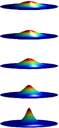
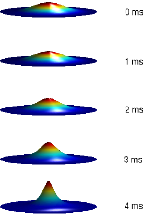
Figure 4: A direct comparison of the collapse between the Gross-Pitaevskii (left) and the resonance approach (right) within the regime of applicability of the Gross-Pitaevskii equation. Each horizontal pair is at the same time step with time increasing from top to bottom. As expected we observe no appreciable difference between the two methods.

We now proceed to a more complex situation in which the timescales for the atom-molecule coupling and the collapse dynamics are more compatible. From a numerical point of view, it becomes convenient to increase the resonance width to 1.5 MHz and the detuning to 14 kHz so that the effect of the atom-molecule coupling will appear in the first stage of the collapse. This allows us to form a complete picture of the dynamics involving the atomic collapse and the simultaneous coupling to a coherent molecular field. The numerical calculation is shown as a movie in Fig. 5 for both the condensed and noncondensed components. One sees the formation of a significant fraction of noncondensed atoms–a feature not described within the Gross-Pitaevskii framework. During a time evolution of 0.8 ms the condensate fraction falls to approximately 80% of its initial value, while the noncondensate fraction reaches a peak at around 20%. The amplitude of the scalar field $\phi_{m}$ remains below the 2% level at all times.

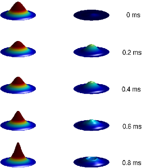
Figure 5: The simulation of the collapse in the resonance theory showing the time evolution of the condensed fraction $\phi_{a}({\mbox{\boldmath$x$}})$ (left) and noncondensed fraction $G_{N}({\mbox{\boldmath$x$}},{\mbox{\boldmath$x$}})$ (right). Each horizontal pair is taken at the same instant of time, with time increasing from top to bottom. It is evident that non condensate atoms are produced during the collapse dynamics, forming rings which propagate from the center of the cloud outward.

To better illustrate the behavior of the atoms during the collapse we present the flow of the different distributions involved. The condensate velocity field is shown in Figure 6. It exhibits similar characteristics to those predicted by the Gross-Pitaevskii theory, which without loss, predicts that the condensed atoms will always accelerate toward the trap center. In contrast, the velocity field of the atoms outside of the condensate is radially outward. The production of this component is quite interesting because it is this same component which in the theory of the Ramsey fringe experiment was quantitatively determined to give rise to the burst.

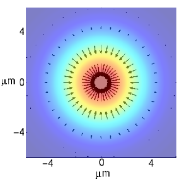
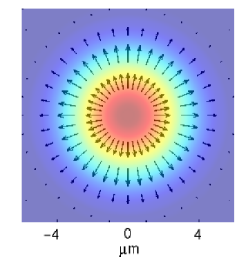
Figure 6: The velocity fields for the condensate component $\phi_{a}({\mbox{\boldmath$x$}})$ (left) and the noncondensed component $G_{N}({\mbox{\boldmath$x$}},{\mbox{\boldmath$x$}})$ (right) midway through the simulation (0.4 ms). The color contours indicate the densities and the velocity fields are represented in direction and strength by the arrows. This clearly shows, that in the resonance theory, as the condensate collapses inward, the noncondensate atoms that are generated flow outward.

Obviously an important quantity to calculate for these expanding noncondensed atoms is the effective temperature, or energy per particle, since this quantity is observed experimentally. This is illustrated in Figure 7 where superimposed on an illustration of the density is a colormap of the temperature. The hottest atoms generated in the center of the cloud are of comparable energy scale to that seen in the experiment, being on the order of 100 nK.

Figure 7: Density distribution of the noncondensate atoms near the end of the simulation (0.8 ms) on which we have superimposed the energy per particle as a colormap. The range of energies, of order 100 nK, is consistent with the characteristic scale of the burst particle energies in the Bosenova experiment. Note that hot atoms are generated in the center of the cloud during the atom-molecule oscillations since this is where the atom-molecule coupling is strongest (the coupling strength varies as the square root of the density). As the hot particles radiate outward a ring can be observed.

4 Conclusion

We emphasize that the work presented here is a model calculation to illustrate the feasibility for the burst to be generated through atom-molecule coupling. However, there are a number of important distinctions with the experimental situation which would have to be accounted for before making a direct comparison. These simulations contain no inelastic three-body loss and particle number is absolutely conserved. In reality three-body loss may be important to the experiment, but we suggest with this work that three-body loss is not the only mechanism for producing a noncondensed burst during the collapse.

It should be emphasized that if our hypothesis for the burst generation is correct, the noncondensate atoms that are produced by this mechanism are not simply generated in a thermal component, but are instead generated in a fundamentally intriguing quantum state. The process of dissociation of molecules into atom pairs produces macroscopic correlations reminiscent of a squeezed vacuum state in quantum optics. This means that every atom in the burst with momentum $k$ would have an associated partner with momentum $-{\mbox{\boldmath$k$}}$. In principle, the correlations could be directly observed in experiments through coincidence measurements providing clear evidence as to whether this is the dominant mechanism for the burst generation in the Bosenova.

5 Acknowledgements

We would like to thank Servaas Kokkelmans and Lincoln Carr for discussions. M.H. and J.M. were supported by the U.S. Department of Energy, Office of Basic Energy Sciences via the Chemical Sciences, Geosciences and Biosciences Division, and C.M. by the National Science Foundation and by the Divisione Cooperazione e Mobilità Internazionale of the University of Trento.

References

References

- [1] Donley E A, Claussen N R, Cornish S L, Roberts J L, Cornell E A and Wieman C E 2001 Nature 412 295
- [2] Duine R A and Stoof H T C 2001 Phys. Rev. Lett. 86 2204
- [3] Santos L and Shlyapnikov G V 2002 Phys. Rev. A. 66 011602
- [4] Saito H and Ueda M 2002 Phys. Rev. A 65 033624
- [5] Savage C M, Robins N P and Hope J J 2003 Phys. Rev. A 67 014304
- [6] Jeon G S, Yin L, Rhee S W and Thouless D J 2002 Phys. Rev. A 66 011603
- [7] Donley E A, Claussen N R, Thompson S T and Wieman C E 2002 Nature 417 529
- [8] Kokkelmans S J J M F and Holland M J 2002 Phys. Rev. Lett. 89 180401
- [9] Mackie M, Suominen K A and Javanainen J 2002 Phys. Rev. Lett. 89 180403
- [10] Köhler T, Gasenzer T and Burnett K 2003 Phys. Rev. A 67 013601
- [11] Chiofalo M L, Kokkelmans S J J M F, Milstein J N and Holland M J 2002 Phys. Rev. Lett. 88 090402
- [12] Kokkelmans S J J M F, Milstein J N, Chiofalo M L, Walser R and Holland M J 2002 Phys. Rev. A 65 053617