Lower bound for electron spin entanglement from beamsplitter current correlations

Abstract

We determine a lower bound for the entanglement of pairs of electron spins injected into a mesoscopic conductor. The bound can be expressed in terms of experimentally accessible quantities, the zero-frequency current correlators (shot noise power or cross-correlators) after transmission through an electronic beam splitter. The effect of spin relaxation ($T_{1}$ processes) and decoherence ($T_{2}$ processes) during the ballistic coherent transmission of the carriers in the wires is taken into account within Bloch theory. The presence of a variable inhomogeneous magnetic field allows the determination of a useful lower bound for the entanglement of arbitrary entangled states. The decrease in entanglement due to thermally mixed states is studied. Both the entanglement of the output of a source (entangler) and the relaxation ($T_{1}$) and decoherence ($T_{2}$) times can be determined.

Quantum nonlocality has been an intriguing issue since the early days of quantum mechanics EPR . Nonlocal effects can come into play when a quantum system is composed of at least two subsystems which are spatially separated. Despite their simplicity, the Bell states of two distant quantum two-state subsystems (A and B)

$${|\Psi_{\pm}\rangle}=\frac{1}{\sqrt{2}}\left({|\!\uparrow\downarrow\rangle}\pm{|\!\downarrow\uparrow\rangle}\right),$$ (1)

$${|\Phi_{\pm}\rangle}=\frac{1}{\sqrt{2}}\left({|\!\uparrow\uparrow\rangle}\pm{|\!\downarrow\downarrow\rangle}\right),$$ (2)

exhibit the essential phenomenology of quantum nonlocality (e.g., they violate Bell’s inequalities Bell ) thus providing an ideal testing ground for quantum nonlocality. Here, we represent the two-state systems as spins 1/2 with basis states “spin up” ${|\!\uparrow\rangle}$ and “spin down” ${|\!\downarrow\rangle}$ with respect to an arbitrary fixed direction in space.

With the development of quantum information theory BD , and in particular with quantum communication, it has become clear that EPR pairs can also play the role of a resource for operations that are impossible with purely classical means. In this context, two-state systems are referred to as quantum bits (qubits), and quantum nonlocality is related to the concept of entanglement (defined below). A number of quantum information processes–quantum teleportation teleportation , quantum key distribution qkd , quantum dense coding qdc , etc.–have been successfully implemented using pairs of photons with entangled polarizations, i.e., in states such as Eqs. (1) and (2). Photons have the advantage that they are easily moved form one place to another, allowing for experiments involving space-like separations between detection events Bell .

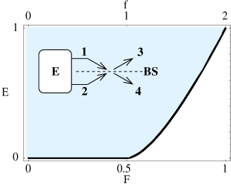
Figure 1: Inset: Proposed setup with two-electron scattering at a beamsplitter (BS) with transmittivity $T$. Electrons are injected pairwise from the entangler (E) into contacts 1 and 2 of the BS. The mean current $I=\langle I_{\alpha}\rangle$ and one of the current correlators $S_{\alpha\beta}$ are measured at the outgoing contacts $\alpha,\beta=3,4$. Plot: Entanglement of formation $E$ of the electron spins versus singlet fidelity $F$ and the reduced correlator $f=S_{33}/2eIT(1-T)$. The curve illustrates the relation between noise and entanglement for Werner states. For general states, the curve represents a lower bound for the entanglement, i.e. allowed values for $E$ and $f$ (or, equivalently, $F$) are represented by points in the shaded region. Measuring $f$ determines a lower bound for the entanglement $E$.

More recently, there has been increasing interest in the use of the spin of electrons in a solid-state environment for spin-based electronics Springer and as qubits for quantum computing LD . Subsequently, quantum communication on a mesoscopic scale, typically on the order of micrometers in semiconductor structures (e.g. quantum wires), was proposed MMM . Rather than achieving space-like separation between detection events on the two sites (this would require sub-picosecond detection), the idea here is to use quantum entanglement between parts of a coherently operating solid-state device (in the most extreme case, a quantum computer). It is then relevant to study the transport of spin-entangled electrons in a many-electron system and possible means of entanglement detection. Two-particle interference at a beam-splitter (BS) combined with the measurement of current fluctuations BLS (in general, the full counting statistics FCS ) was identified as a detector for entanglement.

In this paper, we go one step further, providing a lower bound for the amount $E$ of spin entanglement carried by individual pairs of electrons, related to the zero-frequency current correlators when measured in a BS setup (Fig. 1, Inset) by injecting the electrons separately into the two ingoing leads (1 and 2) and measuring either the current autocorrelator $S_{\alpha\alpha}$ in one of the outgoing leads ($\alpha=3,4$) or the cross-correlator $S_{34}$. It is assumed that the size of the scattering region is smaller than both the coherence length and the mean free path, allowing for ballistic and coherent transport. In the following, $T$ will denote the transmittivity of the BS, i.e. the probability to be scattered from lead $1$ to lead $4$ (or from $2$ to $3$). The ideal BS for the proposed setup does not give rise to backscattering (e.g. from lead 1 back into lead 1, or from 1 into 2, etc.). We will also analyze the effect of such backscattering processes, as they give rise to background shot noise which is unrelated to entanglement. During their transport, the electron spins will be exposed to decoherence and relaxation due to spin-dependent scattering caused by magnetic impurities, nuclear spins, or the spin-orbit coupling (see Flatte for a review). We include these effects within a Bloch equation formalism Slichter . Comparison between our theory and experiment will (i) test proposed entanglers RSL ; LMB ; RL ; Bena ; Bouchiat ; Oliver ; SL and (ii) determine spin relaxation ($T_{1}$) and decoherence ($T_{2}$) times.

The materials and structures required for testing our theory, although at the forefront of current capabilities, appear to be feasible. The largest efforts seem to be necessary to realize the electron spin entangler BLS for which there exists a number of theoretical ideas, using normal–RSL ; LMB or carbon-nanotube–superconductor junctions RL ; Bena ; Bouchiat , or single Oliver , or coupled quantum dots BLS ; SL . The electronic BS and the measurement of BS current correlators have been experimentally demonstrated in a GaAs/AlGaAs heterostructure Liu . Coherent transport of electron spins over more than $100\,\mu{\rm m}$ in GaAs has been observed Kikkawa .

Traditionally, current correlations, and in particular the quantum partition (shot) noise have been used to gain information about a scatterer beyond its conductance Blanter-Buttiker . Here, we use a known scatterer (the BS) to gain information about the quantum state (more precisely, its entanglement) of the scattered particles. The correlation function between the currents $I_{\alpha}(t)$ and $I_{\beta}(t)$ in two leads $\alpha,\beta=1,..,4$ of the BS is defined as

$$S_{\alpha\beta}(\omega)=\lim_{\tau\rightarrow\infty}\frac{h\nu}{\tau}\int_{0}^{\tau}\!\!\!dt\,\,e^{i\omega t}\,{\rm Re}\,\mathrm{Tr}\left[\delta I_{\alpha}(t)\delta I_{\beta}(0)\chi\right],$$ (3)

where $\delta I_{\alpha}=I_{\alpha}-\langle I_{\alpha}\rangle$, $\langle I_{\alpha}\rangle=\mathrm{Tr}(I_{\alpha}\chi)$, $\nu$ is the density of states in the leads, and $\chi$ is the density matrix of the injected electron pair (below, we suppress the orbital part of $\chi$, see BLS for Coulomb effects). Writing $\chi$ in the Bell basis, Eqs. (1) and (2), $\chi=F{|\Psi_{-}\rangle}{\langle\Psi_{-}|}+G_{0}{|\Psi_{+}\rangle}{\langle\Psi_{+}|}+\sum_{i=\pm}G_{i}{|\Phi_{i}\rangle}{\langle\Phi_{i}|}$, and $S_{\alpha\beta}\equiv S_{\alpha\beta}(\omega=0)$, we arrive at

$$S_{\alpha\beta} = FS_{\alpha\beta}^{{|\Psi_{-}\rangle}}+G_{0}S_{\alpha\beta}^{{|\Psi_{+}\rangle}}+\sum_{i=\pm}G_{i}S_{\alpha\beta}^{{|\Phi_{i}\rangle}},\quad\quad$$ (4)

$$S_{\alpha\beta}^{{|\Psi\rangle}} \equiv \lim_{\tau\rightarrow\infty}\frac{h\nu}{\tau}\int_{0}^{\tau}\!\!\!dt\,{\rm Re}\,{\langle\Psi|}\delta I_{\alpha}(t)\delta I_{\beta}(0){|\Psi\rangle}.$$ (5)

Using the standard scattering approach Blanter-Buttiker , we have found earlier BLS that the singlet state ${|\Psi_{-}\rangle}$ gives rise to enhanced shot noise (and cross-correlators) at zero temperature, $S^{{|\Psi_{-}\rangle}}_{33}=-S^{{|\Psi_{-}\rangle}}_{34}=2eIT(1-T)f$, with the reduced correlator $f=2$, as compared to the “classical” Poissonian value $f=1$ noise-review . The average currents are given by $I=\langle I_{3}\rangle=\langle I_{4}\rangle=e/h\nu$. We also know that all triplet states are noiseless, $S^{{|\Psi_{+}\rangle}}_{\alpha\beta}=S^{{|\Phi_{\pm}\rangle}}_{\alpha\beta}=0$ ($\alpha,\beta=3,4$). Both the current autocorrelations (shot noise) and cross-correlations are only due to the singlet component of the incident two-particle wavefunction,

$$S_{33}=-S_{34}=FS^{{|\Psi_{-}\rangle}}=2eIT(1-T)f,\quad f=2F.$$ (6)

Including backscattering with probability $R_{B}$, we find

$$S_{33} = 2eI\left[\,2F(1-R_{B})\,T(1-T)+R_{B}/2\,\right],$$ (7)

$$S_{34} = -2eI\,2F(1-R_{B})\,T(1-T),$$ (8)

where $I=(e/h\nu)(1-R_{B})$. Since $f^{\prime}=S_{34}/2eIT(1-T)=2F(1-R_{B})\leq f$ is smaller than $f$ without backscattering and the entanglement of formation $E$ is a monotonic function of $f$ (see below and Fig. 1), we still obtain a lower bound on $E$ (the bound will become less informative as $R_{B}$ increases). Note that this does not hold for the autocorrelator $S_{33}$. However, one can determine $R_{B}$, e.g. by measuring the shot noise power using normal Fermi lead inputs Liu and then obtain $f$ from either $S_{33}$ or $S_{34}$.

The entanglement of a bipartite state $\chi\in{\cal H}_{A}\otimes{\cal H}_{B}$ can be quantified by its entanglement of formation BDSW $E(\chi)=\min_{\{({|\chi_{i}\rangle},p_{i})\}\in\cal{E}(\chi)}\sum_{i}p_{i}S_{N}({|\chi_{i}\rangle})$, where $\cal{E}(\chi)$ denotes the set of ensembles $\{({|\chi_{i}\rangle},p_{i})\}$ for which $\chi=\sum_{i}p_{i}{|\chi_{i}\rangle}{\langle\chi_{i}|}$. We have used the von Neumann entropy of the reduced density matrix $\rho_{B}=\mathrm{Tr}_{A}{|\psi\rangle}{\langle\psi|}$, $S_{N}({|\psi\rangle})=-\mathrm{Tr}_{B}\rho_{B}\log\rho_{B}$ (logarithms are in base 2). A state with $E>0$ ($E=1$) is (maximally) entangled, whereas a state with $E=0$ is separable (in the case of a pure state, it is a product $\psi_{A}\otimes\psi_{B}$). The Bell states Eq. (1) and (2) are maximally entangled. Neither local operations nor classical communication (LOCC) between subsystems A and B can increase $E$. In quantum information theory, $E(\chi)$ is the maximal ratio $N/M$ of the number $N$ of EPR pairs (maximally entangled states) required to form $M$ copies of $\chi$ as $N\rightarrow\infty$; $E$ is the quantity that measures how much of the resource (quantum entanglement) is available.

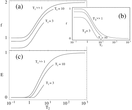
Figure 2: Homogeneous magnetic field $\delta h=0$ and $\tilde{P}=1$. (a) $f$ of the spin singlet state ${|\Psi_{-}\rangle}$ after ballistic transmission through a BS as a function of the spin decoherence time $T_{2}$, in units of the ballistic transmission time $t_{0}=L/v_{F}$. Different curves correspond to different values of the spin relaxation time $T_{1}$ (same units). Note that we only plotted the curves for $T_{2}\leq 2T_{1}$. (b) $f$ for a spin triplet state ${|\Psi_{+}\rangle}$. Since $f\leq 1$, the lower bound on entanglement is zero, i.e. we cannot learn anything about entanglement of injected triplets at $\delta h=0$. (c) Lower bound on the entanglement of formation $E$.

For arbitrary $\chi$, $E(\chi)$ cannot be expressed as a function of only its singlet fidelity $F={\langle\Psi_{-}|}\chi{|\Psi_{-}\rangle}$. However, this is possible for the so-called Werner states Werner

$$\rho_{F}\!=\!F{|\Psi_{-}\rangle}{\langle\Psi_{-}|}\!+\!\frac{1\!-\!F}{3}\!\left({|\Psi_{+}\rangle}{\langle\Psi_{+}|}\!+\!\sum_{i=\pm}{|\Phi_{i}\rangle}{\langle\Phi_{i}|}\right)\!,$$ (9)

being the unique rotationally invariant states with singlet fidelity $F$. It is known BDSW that $E(F)\equiv E(\rho_{F})=H_{2}(1/2+\sqrt{F(1-F)})$ if $1/2<F\leq 1$ and $E(F)\equiv E(\rho_{F})=0$ if $0\leq F<1/2$, with the dyadic Shannon entropy $H_{2}(x)=-x\log x-(1-x)\log(1-x)$. Together with Eq. (6), this enable us to express the entanglement of $\rho_{F}$ in terms of the reduced correlator $f$ (Fig. 1).

We generalize this result to arbitrary mixed states $\chi$ of two spins (qubits). Any state $\chi$ can be transformed into the Werner state $\rho_{F}$ with the same singlet fidelity $F$ by a random bipartite rotation BBPSSW ; BDSW , i.e. by choosing a random $U\in SU(2)$ and applying $U\otimes U$ to $\chi$. Since this operation involves only LOCC, $E$ cannot increase,

$$E(F)\leq E(\chi).$$ (10)

The entanglement of formation $E(F)$ of the corresponding Werner state therefore provides a lower bound on the entanglement of $\chi$ (Fig.1). Thus, a noise signal exceeding the Poissonian limit ($f>1$) in the BS setup can in principle be interpreted as a sign of entanglement between the electron spins injected into leads 1 and 2 .

We now include relaxation and decoherence into our analysis. At time $t=0$, we start with a spin singlet (upper sign) or triplet (lower sign) state

$$\chi(0)={|\Psi_{\mp}\rangle}{\langle\Psi_{\mp}|}.$$ (11)

We describe the dynamics of $\chi(t)$ in a field $\mathbf{B}\parallel\hat{z}$ and in the presence of spin decoherence ($T_{2}$ processes) and relaxation ($T_{1}$) phenomenologically within a single-spin Bloch equation for the polarization $\mathbf{P}=(\langle\sigma_{x}\rangle,\langle\sigma_{y}\rangle,\langle\sigma_{z}\rangle)$,

$$\dot{\mathbf{P}}=\mathbf{P}\times\mathbf{h}-R(\mathbf{P}-\tilde{\mathbf{P}})\equiv-\Omega(\mathbf{P}-\tilde{\mathbf{P}}),$$ (12)

with $\langle\sigma_{i}\rangle=\mathrm{Tr}(\sigma_{i}\rho)$, $\mathbf{h}=g\mu_{B}\mathbf{B}=(0,0,h)$, the stationary polarization $\tilde{\mathbf{P}}=(0,0,\tilde{P})$ (note that $\tilde{\mathbf{P}}\times\mathbf{h}=0$), and the relaxation matrix $R_{ij}=\delta_{ij}R_{i}$ with $R_{1}=R_{2}=T_{2}^{-1}$ and $R_{3}=T_{1}^{-1}$. Solving Eq. (12), we obtain

$$\mathbf{P}(t)=e^{-\Omega t}\mathbf{P}(0)+(1-e^{-\Omega t})\tilde{\mathbf{P}},$$ (13)

or, in terms of the spin density matrix,

$$\rho(t)=(P_{0}+\mathbf{P}(t)\cdot\mbox{\boldmath$\sigma$})/2\equiv\Lambda_{h}(t)[\rho(0)],$$ (14)

with the superoperator ($a(t)=1-e^{-t/T_{1}}$)

$$\Lambda_{h}(t)[\rho]=\left(\begin{array}[]{c c}\frac{1}{2}(\rho_{\uparrow\uparrow}+\rho_{\downarrow\downarrow})(1+a(t)\tilde{P})+\frac{1}{2}(\rho_{\uparrow\uparrow}-\rho_{\downarrow\downarrow})e^{-t/T_{1}}&e^{-t/T_{2}+iht}\rho_{\uparrow\downarrow}\\ e^{-t/T_{2}-iht}\rho_{\downarrow\uparrow}&\frac{1}{2}(\rho_{\uparrow\uparrow}+\rho_{\downarrow\downarrow})(1-a(t)\tilde{P})-\frac{1}{2}(\rho_{\uparrow\uparrow}-\rho_{\downarrow\downarrow})e^{-t/T_{1}}\end{array}\right),$$ (15)

with the matrix elements $\rho_{ij}=\langle i|\rho|j\rangle$ and $(i,j=\uparrow,\downarrow)$. We apply $\Lambda_{h}(t)$ to both spins individually,

$$\chi(t)=\left(\Lambda_{h_{1}}(t)\otimes\Lambda_{h_{2}}(t)\right)[\chi(0)],$$ (16)

where $h_{i}$ is the field at electron $i$. Using Eq. (6) and $F(t)={\langle\Psi_{-}|}\chi(t){|\Psi_{-}\rangle}$ at time $t\geq 0$, we obtain

$$f(t) = \pm e^{-2t/T_{2}}\cos(\delta h\,t)$$ (17)

$$+\frac{1}{2}(1+e^{-2t/T_{1}})-\frac{1}{2}(1-e^{-t/T_{1}})^{2}\tilde{P}^{2},$$

where $\delta h=h_{1}-h_{2}$. If the decoherence time $T_{2}^{(1,2)}$ of the two electrons is different, then $T_{2}$ in Eq. (17) becomes $T_{2}^{\rm EPR}=(1/T_{2}^{(1)}+1/T_{2}^{(2)})^{-1}$. We define $T_{1}^{\rm EPR}$ similarly if $\tilde{P}=0$. However, if $\tilde{P}=1$, then $\exp(-t/T_{1})$ is replaced by $\exp(-t/T_{1}^{(1)})+\exp(-t/T_{1}^{(2)})$.

A homogeneous field, $\delta h=0$, does not affect $f$. For slow relaxation, $T_{1}\gg t$, we find $f(t)=1\pm e^{-2t/T_{2}}$. In Fig. 2a we plot $f$ for $\delta h=0$ and $\tilde{P}=1$ versus $T_{2}$ in units of the ballistic transmission time noise-review $t_{0}=L/v_{F}$ ($L$=length of ballistic trajectory, $v_{F}$=Fermi velocity). For unentangled triplet states, $\chi(0)={|\!\uparrow\uparrow\rangle}{\langle\uparrow\uparrow\!|},{|\!\downarrow\downarrow\rangle}{\langle\downarrow\downarrow\!|}$, we find $f\leq 1/2$ for all $T_{1}$, $T_{2}$, and $\tilde{P}$ (Fig. 2b).

An inhomogeneous field $\delta h\neq 0$ (or, equivalently, a local controllable Rashba spin-orbit coupling EBL ) has the effect of continuously rotating singlets into triplets and vice versa (Fig. 3). This a lower bound of the triplet entanglement, $\chi(0)={|\Psi_{+}\rangle}{\langle\Psi_{+}|}$, which is as tight as Eq. (10) for the singlet,

$$E\geq\max_{\delta{\bf h}}E\left(f\left(\delta{\bf h}\right)/2\right),$$ (18)

where $f(\delta{\bf h})$ is the measured noise power (or cross-correlator), $E(F)$ is the entanglement of the Werner state $\rho_{F}$ (Fig. 1). If a field inhomogeneity $\delta{\bf h}$ can be created pointing in arbitrary directions in space, then the above result represents a tight lower bound for any injected entangled state. In particular, each maximally entangled state ${|\Psi\rangle}$ will be detected in this way, since there exists a $u=\exp(-i\delta{\bf h}\cdot\mbox{\boldmath$\sigma$})\in SU(2)$ such that $u^{\dagger}\otimes u{|\Psi\rangle}={|\Psi_{-}\rangle}$. This rotation can also be done unilaterally, i.e. there is a $v\in SU(2)$ with $v\otimes 1{|\Psi\rangle}={|\Psi_{-}\rangle}$ (see also EBL ).

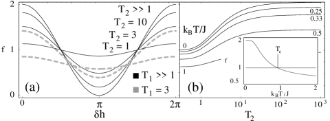
Figure 3: (a) Reduced current correlator $f$ versus field inhomogeneity $\delta h=h_{1}-h_{2}$ (in units of $\hbar/t_{0}g\mu_{B}$, $t_{0}$=ballistic transmission time, $g$=g-factor, $\mu_{B}$=Bohr magneton) for an injected singlet state and $\tilde{P}=1$. Solid lines represent $T_{1}\gg 1$ and $T_{2}=1,3,10,\infty$, grey dashed lines $T_{1}=3$ and $T_{2}=1,3$. For injected triplets, the plot is phase-shifted by $\pi$, providing tight lower bounds at $\delta h=\pi$. Tight lower bounds for any input state can be determined by varying the direction of $\delta{\mathbf{h}}$. (b) Plot of $f$ for a thermally mixed initial state versus $T_{2}$ (in units of $t_{0}$) for $T_{1}\gg t$ and $\tilde{P}=1$. The various curves correspond to $k_{B}\mathrm{T}/J=0,0.25,0.33,0.5,1$, where $J$ and $\mathrm{T}$ denote the exchange energy and temperature during the preparation of the state. Inset: The maximal $f$ (at $T_{1},T_{2}\gg t_{0}$) versus $k_{B}\mathrm{T}/J$. There is no entanglement ($f\leq 1$, $E=0$) above the critical temperature $\mathrm{T}_{c}=0.91\,J/k_{B}$.

Finally, we study the case where the spin state of the injected pair of carriers Eq. (11) is mixed, because it is prepared at a temperature $\mathrm{T}$ comparable to the energy splitting between spin states, typically (if the Zeeman effect is negligible) the exchange energy $J$, i.e. the singlet-triplet splitting. In this case, $\chi(0)=\rho_{F}$ with $F=(1+3e^{-J/k_{B}\mathrm{T}})^{-1}$ where $k_{B}$ is Boltzmann’s constant. We only show the resulting $f$ for $T_{1}\gg t$ here (the full expression will be reported elsewhere unpublished ),

$$f(t)=\frac{1+e^{-2t/T_{2}}+e^{-J/k_{B}\mathrm{T}}\left(1-e^{-2t/T_{2}}\right)}{1+3e^{-J/k_{B}\mathrm{T}}},$$ (19)

which is the statistical mixture of Eq. (17) for the singlet and triplet with the appropriate Boltzmann weights (Fig. 3b). Above the critical temperature $\mathrm{T}_{c}=0.91\,J/k_{B}$ there is no entanglement even for $T_{1},T_{2}\rightarrow\infty$.

Acknowledgments: We thank D. P. DiVincenzo and B. M. Terhal for valuable discussions. DL acknowledges funding from the Swiss NSF, NCCR Nanoscience, and DARPA QUIST and SPINS.

References

(1)
A. Einstein, B. Podolski, and N. Rosen, Phys. Rev. 47, 777 (1935).
(2)
J. S. Bell, Rev. Mod. Phys. 38, 447 (1966);
A. Aspect, J. Dalibard, G. Roger,
Phys. Rev. Lett. 49, 1804 (1982).
(4)
C. H. Bennett et al.,
Phys. Rev. Lett. 70, 1895 (1993);
D. Boumeester et al., Nature 390, 575 (1997);
D. Boschi et al.,
Phys. Rev. Lett. 80, 1121 (1998).
(5)
A. K. Ekert,
Phys. Rev. Lett. 67, 661 (1991).
(6)
K. Mattle et al.,
Phys. Rev. Lett. 76, 4656 (1996).
(7)Semiconductor Spintronics and Quantum Computation,
eds. D. D. Awschalom, D. Loss, and N. Samarth
(Springer, Berlin, 2002).
(8)
D. Loss, D. P. DiVincenzo, Phys. Rev. A 57, 120 (1998).
(9)
D. V. DiVincenzo and D. Loss,
J. Mag. Magn. Matl. 200, 202 (1999) [cond-mat/9901137].
(10)
G. Burkard, D. Loss, and E. V. Sukhorukov,
Phys. Rev. B 61, R16303 (2000)
[cond-mat/9906071].
(11)
F. Taddei and R. Fazio, Phys. Rev. B 65, 075317 (2002).
(12)
M. E. Flatté, J. M. Byers, W. H. Lau, Chap. 4 in Ref. Springer .
(13)
C. P. Slichter, Princliples of Nuclear Magnetic Resonance,
3rd ed. (Springer, Berlin, 1990).
(14)
P. Recher, E. V. Sukhorukov, and D. Loss,
Phys. Rev. B 63, 165314 (2001).
(15)
G. B. Lesovik, T. Martin, and G. Blatter,
Eur. Phys. J. B 24, 287 (2001).
(16)
P. Recher and D. Loss,
Phys. Rev. B 65, 165327 (2002).
(17)
C. Bena et al.,
Phys. Rev. Lett. 89, 037901 (2002).
(18)
V. Bouchiat et al., cond-mat/0206005.
(19)
W. D. Oliver, F. Yamaguchi, and Y. Yamamoto,
Phys. Rev. Lett. 88, 037901 (2002).
(20)
D. Saraga and D. Loss, cond-mat/0205553.
(21)
R. C. Liu et al.,
Nature (London), 391, 263 (1998).
(22)
J. M. Kikkawa and D. D. Awschalom,
Nature 397, 139 (1999).
(23)
Ya. M. Blanter, M. Büttiker,
Phys. Rep. 336, 1 (2000).
(24)
For a discussion of the range of validity of this result
and an estimate of the ballistic transfer time , see
Section 9 in
J. C. Egues et al., cond-mat/0210498.
(25)
C. H. Bennett et al.,
Phys. Rev. A 54, 3824 (1996).
(26)
R. F. Werner, Phys. Rev. A 40, 4277 (1989).
(27)
C. H. Bennett et al.,
Phys. Rev. Lett. 76, 722 (1996).
(28)
J. C. Egues, G. Burkard, and D. Loss,
Phys. Rev. Lett. 89, 176401 (2002).