Bogoliubov spectrum and Bragg spectroscopy
of elongated Bose-Einstein condensates

Abstract

The behavior of the momentum transferred to a trapped Bose-Einstein condensate by a two-photon Bragg pulse reflects the structure of the underlying Bogoliubov spectrum. In elongated condensates, axial phonons with different number of radial nodes give rise to a multibranch spectrum which can be resolved in Bragg spectroscopy, as shown by Steinhauer et al. [Phys. Rev. Lett. 90, 060404 (2003)]. Here we present a detailed theoretical analysis of this process. We calculate the momentum transferred by numerically solving the time dependent Gross-Pitaevskii equation. In the case of a cylindrical condensate, we compare the results with those obtained by linearizing the Gross-Pitaevskii equation and using a quasiparticle projection method. This analysis shows how the axial-phonon branches affect the momentum transfer, in agreement with our previous interpretation of the observed data. We also discuss the applicability of this type of spectroscopy to typical available condensates, as well as the role of nonlinear effects.

I Introduction

In a recent paper steinhauer2003 we showed that interesting features emerge in the momentum transferred to an elongated Bose-Einstein condensate by a two-photon Bragg pulse when the duration of the pulse is long enough. On the basis of numerical simulations with the Gross-Pitaevskii (GP) equation, we interpreted those features as due to the structure of the underlying Bogoliubov spectrum: the Bragg pulse can excite axial phonons with different number of radial nodes, each one having its dispersion law. Since the energy difference between these branches is of the order of the radial trapping frequency, they can be resolved only by Bragg pulses with duration comparable with the radial trapping period, as observed in steinhauer2003 . In this work, we present a more detailed theoretical analysis that supports our previous interpretation and gives further information about the role played by Bogoliubov excitations in Bragg spectroscopy.

A useful insight into this problem is obtained by studying the case of an infinite condensate, unbound along $z$ and harmonically trapped in the radial direction $\rho$. We show that the response of such a cylindrical condensate retains all the relevant properties needed to interpret the observed behavior of a finite elongated condensate. In addition to the numerical solution of the full time dependent GP equation, we explicitly determine the time evolution of the order parameter in the linear (small amplitude) limit, using the quasiparticle projection method of Refs. morgan ; bbg . The cylindrical geometry allows us to simplify the calculations and, more important, to make the connection between the momentum transferred and the dynamic structure factor more direct than for a finite condensate. By comparing the predictions of this approach to the results of the numerical integration of the time dependent GP equation, one can also distinguish the different effects of linear and nonlinear dynamics. This analysis of cylindrical condensates is presented in the first sections of this paper, while section V is devoted to the behavior of finite elongated condensates, as the ones in the experiments of Refs. steinhauer2003 ; mit ; rehovot .

II Bogoliubov spectrum of a cylindrical condensate

First we investigate the excitation spectrum of a cylindrical condensate. We use the mean-field Gross-Pitaevskii theory at zero temperature, assuming the condensate to be dilute and cold enough to neglect thermal and beyond mean-field contributions. The starting point is the time dependent GP equation for the order parameter $\Psi({\bf r},t)$ of a condensate of $N$ bosonic atoms subject to an external potential $V({\bf r})$ rmp :

$$i\hbar\frac{\partial}{\partial t}\Psi=\left(-\frac{\hbar^{2}\nabla^{2}}{2m}+V+g|\Psi|^{2}\right)\Psi\;,$$ (1)

where $g=4\pi\hbar^{2}a/m$, and $a$ is the $s$-wave scattering length, that we assume to be positive. The order parameter is normalized according to $\int d{\bf r}|\Psi|^{2}=N$. What is usually named Bogoliubov spectrum is the result of an expansion of $\Psi$ in terms of a quasiparticles basis in the form bogoliubov ; pitaevskii ; fetter :

$$\Psi({\bf r},t) = e^{-i\mu t/\hbar}\{\psi_{0}({\bf r})+$$ (2)

$$\sum_{j} [c_{j}u_{j}({\bf r})e^{-i\omega_{j}t}+c_{j}^{*}v_{j}^{*}({\bf r})e^{i\omega_{j}t}]\}\;,$$

where the $c_{j}$’s are constants and $\mu$ is the chemical potential. The quasiparticle amplitudes $u$ and $v$ obey the following orthogonality and symmetry relations:

$$\int\!d{\bf r}\{u_{i}u_{j}^{*}-v_{i}v_{j}^{*}\}=\delta_{ij}\;\;;\;\;\int\!d{\bf r}\{u_{i}v_{j}-v_{i}u_{j}\}=0\;.$$ (3)

This expansion can be inserted into Eq. (1). At zero order in $u$ and $v$, one gets the stationary GP equation:

$$\left(-\frac{\hbar^{2}\nabla^{2}}{2m}+V({\bf r})+g|\psi_{0}({\bf r})|^{2}\right)\psi_{0}({\bf r})=\mu\psi_{0}({\bf r})\;.$$ (4)

Among the solutions of this equation one finds the ground state order parameter, which can be chosen real and equal to the square root of the particle density note-gs . The next order gives the coupled equations

$$\hbar\omega_{i}u_{i} = [H_{0}-\mu+2g\psi_{0}^{2}]u_{i}+g\psi_{0}^{2}v_{i}$$ (5)

$$-\hbar\omega_{i}v_{i} = [H_{0}-\mu+2g\psi_{0}^{2}]v_{i}+g\psi_{0}^{2}u_{i}\;,$$ (6)

where $H_{0}=-(\hbar^{2}/2m)\nabla^{2}+V({\bf r})$. The solutions of these equations provide the spectrum of the excited states in the linear (small amplitude) regime.

Now we treat the specific case of a cylindrical condensate, which is unbound along $z$ and harmonically trapped along the radial direction, $\rho=[x^{2}+y^{2}]^{1/2}$. Let us write the trapping potential as $V({\bf r})=V_{T}(\rho)=(1/2)m\omega_{\rho}^{2}\rho^{2}$. The ground state order parameter is uniform along $z$, while the stationary GP equation for the radial part becomes

$$\left[-\frac{\hbar^{2}\nabla^{2}_{\rho}}{2m}+V_{T}(\rho)+\frac{gN}{L}\phi_{0}^{2}(\rho)\right]\phi_{0}(\rho)=\mu\phi_{0}(\rho)$$ (7)

where $N/L$ is the number of bosons per unit length and the function $\phi_{0}$ is chosen to be real and subject to the normalization condition $2\pi\int_{0}^{\infty}\!d\rho\,\rho\phi_{0}^{2}=1$. In this geometry, the quasiparticle amplitudes $u$ and $v$ can also be factorized. We are actually interested in axially symmetric states (azimuthal angular momentum equal to zero), since they are the only ones excited by a Bragg process in which the momentum is imparted along the $z$-axis. These states, characterized by the axial wavevector, $k$, and the number of radial nodes, $n$, can be written in terms of new functions $u_{n,k}(\rho)$ and $v_{n,k}(\rho)$ in the form

$$(u,v)_{n,k}(\rho,z)=L^{-1/2}e^{ikz}(u,v)_{n,k}(\rho)\;.$$ (8)

The Bogoliubov equations (5)-(6) then become

$$\hbar\omega_{n,k}u_{n,k}(\rho) = \left(-\frac{\hbar^{2}\nabla^{2}_{\rho}}{2m}+\frac{\hbar^{2}k^{2}}{2m}+V_{T}(\rho)-\mu+\frac{2gN}{L}\phi_{0}^{2}(\rho)\right)u_{n,k}(\rho)+\frac{gN}{L}\phi_{0}^{2}(\rho)v_{n,k}(\rho)$$ (9)

$$-\hbar\omega_{n,k}v_{n,k}(\rho) = \left(-\frac{\hbar^{2}\nabla^{2}_{\rho}}{2m}+\frac{\hbar^{2}k^{2}}{2m}+V_{T}(\rho)-\mu+\frac{2gN}{L}\phi_{0}^{2}(\rho)\right)v_{n,k}(\rho)+\frac{gN}{L}\phi_{0}^{2}(\rho)u_{n,k}(\rho)\;.$$ (10)

Numerical solutions of the Bogoliubov equations for cylindrical condensates have already been obtained in the context of theoretical studies of the Landau critical velocity fedichev , the Landau damping of low energy collective oscillations muntsa , and the behavior of solitary waves komineas . Here we solve equations (9)-(10) in order to use the functions $u$ and $v$ as a basis for a time dependent calculation, as explained in the next section.

It is worth noticing that, expressing all lengths and energies in units of the harmonic oscillator length, $a_{\rho}=[\hbar/(m\omega_{\rho})]^{1/2}$, and energy, $\hbar\omega_{\rho}$, respectively, the solutions of GP and Bogoliubov equations for the cylindrical condensate scale with a single parameter, $aN/L$. The same parameter can be expressed in terms of the chemical potential in the Thomas-Fermi limit, $\mu_{\rm TF}$. One has in fact, $\eta\equiv\mu_{\rm TF}/(\hbar\omega_{\rho})=[4aN/L]^{1/2}$ fedichev ; note1 . We perform calculations for different values of $\eta$, which are representative of available elongated condensates. The lowest value that we consider is $\eta=9.4$, which simulates the condensate of Davidson and co-workers steinhauer2003 ; rehovot , the largest value is $\eta=70$, for the condensate of Ref. onofrio . We also use an intermediate value, $\eta=26.5$, which corresponds to the condensate of the calculations in Refs. brunello ; brunello2 .

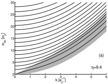
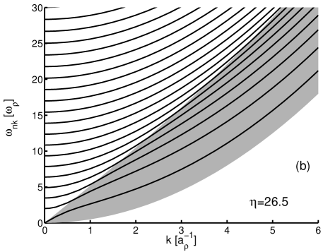
Figure 1: Spectrum of axially symmetric Bogoliubov excitations of cylindrical condensates with $\eta=9.4$ (a) and $\eta=26.5$ (b). The frequency $\omega_{n,k}$, in units of the radial trapping frequency $\omega_{\rho}$, is plotted as a function of the axial wavevector $k$, in units of $a_{\rho}^{-1}$, with $a_{\rho}=[\hbar/(m\omega_{\rho})]^{1/2}$. The number of radial nodes is $n=0,1,2,\dots$, starting from the lowest branch. The shaded area corresponds to the region that gives finite contributions to the the dynamic structure factor $S(q,\omega)$ in local density approximation (see section IV).

In Figs. 1a and 1b we show the frequency $\omega_{n,k}$ of the Bogoliubov branches as a function of $k$, for $\eta=9.4$ and $26.5$, respectively. The lowest branch starts linearly at low $k$ and then becomes quadratic for large $k$, as expected for the textbook Bogoliubov spectrum of a uniform condensate. The transition between the two regimes occurs at $k$ of the order of $\xi^{-1}=\sqrt{\eta}$, where $\xi$ is the healing length. The slope of this branch has been the object of the investigation of Ref. fedichev . The second branch starts at $\omega_{2,0}=2\omega_{\rho}$, where it reduces to the transverse monopole (breathing) mode; its frequency is model independent as a consequence of a scaling property of GP equation in two dimensions pitaevskii97 . For $k\ll\xi^{-1}$ the dispersion law of the lowest branches can be obtained, with great accuracy, also within a hydrodynamic approach hydro .

Our purpose is now to explore the effects of the discrete multibranch spectrum of Figs.1a and 1b in the response of the condensate to a Bragg pulse.

III Time dependent quasiparticle amplitudes and momentum transferred

Let us suppose that a Bragg pulse is switched on at a time $t=0$. In the experiments, this is obtained by shining the condensate with two laser beams with wavevectors ${\bf k}_{1}$ and ${\bf k}_{2}$ and frequencies $\omega_{1}$ and $\omega_{2}$. The action of the stimulated light-scattering from atoms of the condensate is equivalent to a moving optical potential with wavevector ${\bf q}={\bf k}_{1}-{\bf k}_{2}$ and frequency $\omega=\omega_{1}-\omega_{2}$. Within the GP theory, this is accounted for by adding an extra term to the external potential, that becomes blakie

$$V({\bf r},t)=V_{T}(\rho)+\theta(t)V_{B}\cos(qz-\omega t)\,,$$ (11)

where $\theta(t)$ is the Heaviside step function and we have chosen ${\bf q}$ along $z$. We calculate the response of the condensate in two ways: i) by using the quasiparticle projection method of Refs. morgan ; bbg ; ii) by numerically solving the full time dependent GP equation (1) for given values of $\eta,V_{B},q$ and $\omega$. The latter case will be discussed in the next section. Here we briefly sketch the quasiparticle projection method and its application to infinite cylindrical condensates.

The starting point is a generalization of the Bogoliubov expansion (2) that allows the population of quasiparticle states to vary with time morgan . The simplest way is to expand the order parameter in terms of a quasiparticle basis as in (2), but taking the coefficients $c_{j}$ to be time dependent:

$$\Psi({\bf r},t) = e^{-i\mu t/\hbar}\{\psi_{0}({\bf r})+$$ (12)

$$\sum_{j} [c_{j}(t)u_{j}({\bf r})e^{-i\omega_{j}t}+c_{j}^{*}(t)v_{j}^{*}({\bf r})e^{i\omega_{j}t}]\}\;.$$

The functions $\psi_{0}$, $u_{j}$ and $v_{j}$ are the solutions of Eqs.(4)-(6) and are assumed to be static. Let us suppose that at $t=0$ the condensate is in the ground state and thus all $c_{j}(0)$ are zero. For $t>0$ the Bragg potential starts populating the quasiparticle states. The dynamics is entirely fixed by the evolution of the coefficients $c_{j}(t)$, that can be obtained by inserting the expansion (12) into the GP equation (1), with the external potential given in (11). One finds bbg

$$\sum_{j} [ \dot{c}_{j}(t)u_{j}({\bf r})e^{-i\omega_{j}t}+\dot{c}_{j}^{*}(t)v_{j}^{*}({\bf r})e^{i\omega_{j}t}]$$ (13)

$$= \frac{\theta(t)V_{B}}{i\hbar}\ e^{-i\mu t/\hbar}\cos(qz-\omega t)\Psi({\bf r},t)\;.$$

In order to get an expression for the $\dot{c}$’s, one can multiply by $u_{i}^{*}$ and $v_{i}^{*}$ the last equation and its conjugate, respectively, and integrate in $d{\bf r}$. By using the orthogonality and symmetry relations (3) one gets

$$\dot{c}_{i}(t)=\frac{\theta(t)V_{B}}{i\hbar}\ e^{i\omega_{i}t}\int\!d{\bf r} [ u_{i}^{*}e^{i\mu t}\Psi+v_{i}^{*}e^{-i\mu t}\Psi^{*}]$$ (14)

$$\times \cos(qz-\omega t)$$

Finally, assuming that the quasiparticle occupation is always much smaller than $N$, one can replace $\Psi$ with the ground state order parameter and integrate in time. The results is bbg

$$c_{i}(t)=\frac{V_{B}}{i\hbar}\int_{0}^{t}\!dt^{\prime}e^{i\omega_{i}t^{\prime}}\int\!d{\bf r}\ (u_{i}^{*}+v_{i}^{*})\psi_{0}\cos(qz-\omega t^{\prime})$$ (15)

which is expected to be valid in the limit of small perturbations.

In the case of a cylindrical condensate, we can use the factorization (8) to rewrite the previous expression in the form

$$c_{n,k}(t)=\frac{V_{B}2\pi\sqrt{N}}{i\hbar L}\int_{0}^{t}dt^{\prime}\ e^{i\omega_{n,k}t^{\prime}}\int_{0}^{\infty}\!d\rho\ \rho[u^{*}_{n,k}(\rho)$$

$$+v^{*}_{n,k}(\rho)]\phi_{0}(\rho)\int_{-\infty}^{\infty}\!dz\ e^{-ikz}\cos(qz-\omega t^{\prime})\;.$$ (16)

The last integral simply selects out the quasiparticles with $k=\pm q$, so that

$$c_{n,k}(t)=-\frac{\sqrt{N}V_{B}W_{n,k}}{2\hbar}\left[\frac{e^{i(\omega_{n,k}-\omega)t}-1}{\omega_{n,k}-\omega}\delta_{k,q}\right.$$

$$\left.+\frac{e^{i(\omega_{n,k}+\omega)t}-1}{\omega_{n,k}+\omega}\delta_{k,-q}\right]\;,$$ (17)

where

$$W_{n,k}=2\pi\int\!d\rho\ \rho[u^{*}_{n,k}(\rho)+v^{*}_{n,k}(\rho)]\phi_{0}(\rho)\;.$$ (18)

This means that, once the ground state and the Bogoliubov spectrum are known at $t=0$, the order parameter at time $t>0$ can be calculated in a rather simple way.

An important quantity that can easily be calculated within this scheme is the total momentum imparted to the condensate, which can be defined by integrating the current density associated with the order parameter:

$$P_{z}(t)=\frac{\hbar}{2i}\int\!d{\bf r}\ \Psi^{*}({\bf r},t)\frac{\partial}{\partial z}\Psi({\bf r},t)+{\rm c.c.}\;.$$ (19)

By inserting the expansion (12) and using the orthogonality and symmetry relations (3), one gets the simple expression

$$P_{z}(t)=\sum_{n,k}\hbar k\ |c_{n,k}(t)|^{2}\;.$$ (20)

Now, let us take $c_{n,k}(t)$ from Eq. (17) and use the fact that the eigenfrequencies and eigenfunctions of the Bogoliubov equations (9)-(10) are even functions of $k$. One gets the final result

$$P_{z}(t)=\frac{NqV_{B}^{2}t^{2}}{4\hbar}\sum_{n}|W_{n,q}|^{2}\left[\left(\frac{\sin[(\omega_{n,q}-\omega)t/2]}{(\omega_{n,q}-\omega)t/2}\right)^{2}\right.$$

$$\left.-\left(\frac{\sin[(\omega_{n,q}+\omega)t/2]}{(\omega_{n,q}+\omega)t/2}\right)^{2}\right].$$ (21)

In the next section we will show typical results obtained with this expression, but some relevant features are already evident. Notice first that, for positive $\omega$ and a given $q$, the momentum transferred (21) is clearly resonant at the frequencies $\omega=\omega_{n,q}$. In other words, a peak occurs in $P_{z}$ whenever a vertical line at $k=q$ crosses the Bogoliubov branches of Figs. 1a and 1b. The separation between these branches is roughly $1$-$2\ \omega_{\rho}$, while the width of each peak goes like $2\pi/t$. Thus, in order to resolve the different peaks, one has to wait at least a time of the order of trapping period $T_{\rho}=2\pi/\omega_{\rho}$. For $t$ in this range, the second term in the square bracket gives certainly a negligible contribution. Finally, the contribution of each axial branch to the total momentum depends on the quantities $W_{n,q}$, defined in Eq. (18). Typically, for a given $q$, the lowest branches have a greater weight in the summation (21), since the corresponding quasiparticle amplitudes have a greater overlap with the ground state.

This behavior of $P_{z}$ reflects its direct connection with the dynamic structure factor. At zero temperature, the latter is defined as

$$S({\bf q},\omega)=\sum_{i}|\langle i|\hat{\rho}_{\bf q}|0\rangle|^{2}\delta(\omega-\omega_{i})\;,$$ (22)

where $\hat{\rho}_{\bf q}$ is the density fluctuation operator, $|0\rangle$ is the ground state, $|i\rangle$ are the excited states, and $\omega_{i}=(E_{i}-E_{0})/\hbar$. In terms of the quasiparticle amplitudes one has csordas ; zambelli

$$\langle i|\hat{\rho}_{\bf q}|0\rangle=\int\!d{\bf r}\ [u^{*}_{i}({\bf r})+v^{*}_{i}({\bf r})]e^{i{\bf q}\cdot{\bf r}}\psi_{0}({\bf r})\;.$$ (23)

If ${\bf q}$ is taken along $z$, and the system is translational invariant in the same direction, one can use Eqs. (8) and (18) to rewrite $S({\bf q},\omega)$ as

$$S(q,\omega)=\sum_{n}N|W_{n,q}|^{2}\delta(\omega-\omega_{n,q})\,.$$ (24)

Comparing this result with Eq. (21) one finds bbg ; brunello

$$\lim_{t\to\infty}P_{z}(t)=\frac{\pi qV_{B}^{2}t}{2\hbar}[S(q,\omega)-S(-q,-\omega)]\;.$$ (25)

As discussed in Ref. bbg , these two quantities are connected in such a simple way only for a cylindrical condensate. If the condensate is trapped also along $z$, the relation between $S(q,\omega)$ and $P_{z}$ is less direct, involving a further integration on the duration time of the Bragg pulse. However, if the axial trapping frequency is significantly smaller than the radial one, there exists a wide range of time where the connection between the momentum transferred and the dynamic structure factor is roughly the same as for an infinite cylinder. In that range, the Bogoliubov branches, which correspond to $\delta$ peaks in $S(q,\omega)$, are also observable as distinguishable peaks in $P_{z}(t)$, as we will see in section V.

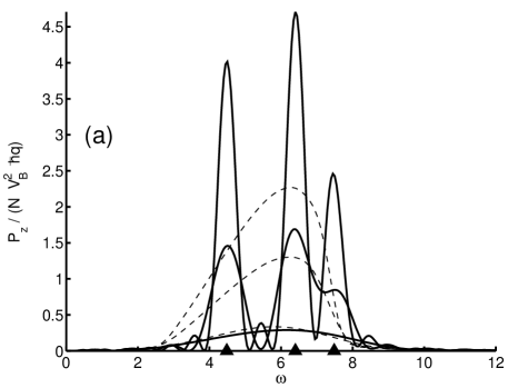
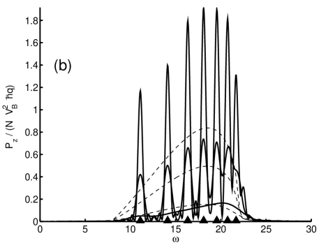
Figure 2: Momentum transferred to cylindrical condensates with $\eta=9.4$ (a) and $\eta=26.5$ (b) by a Bragg pulse of wavevector $q=2.3a_{\rho}^{-1}$ (a) and $q=4\ a_{\rho}^{-1}$ (b), and frequency $\omega$. The quantity $P_{z}/(NV_{B}^{2}\hbar q)$, in units of $(\hbar\omega_{\rho})^{-2}$, is plotted vs. $\omega$, in units of $\omega_{\rho}$. Solid lines correspond to the results obtained from Eq. (21) at three different times, $t=2$ (bottom curve), $6$ (mid) and $10$ (top) $\omega_{\rho}^{-1}$. The dashed lines are the corresponding predictions of the local density approximation. The triangles on the horizontal axis are the frequencies of the lowest Bogoliubov states that contribute to $P_{z}$.

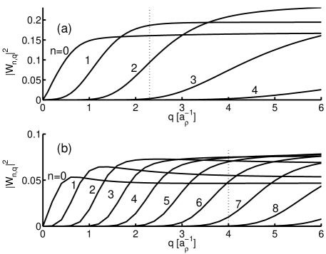
Figure 3: Quantities $|W_{n,q}|^{2}$, defined in Eq.(18), for the two condensates in Fig. 2. In the linear response regime, these functions provide the height of the $\delta$-peaks in the dynamic structure factor (24), as well as of the peaks in the momentum transferred (21). The values of $q$ used in Fig. 2 are shown as vertical dotted lines.

IV Bogoliubov branches and multipeak spectrum

In Figs. 2a and 2b we show the momentum transferred to two cylindrical condensates with $\eta=9.4$ and $26.5$ by a Bragg pulse with wavevector $q=2.3a_{\rho}^{-1}$ (a) and $q=4\ a_{\rho}^{-1}$ (b). Recalling that $\xi^{-1}=\sqrt{\eta}$, the values of $q$ are chosen in order to have roughly the same value of $q\xi$ in the two cases. As solid lines we plot the quantity $P_{z}(t)/(NV_{B}^{2}\hbar q)$ as a function of $\omega$ and for three different durations times: $t=2,6$ and $10\ \omega_{\rho}^{-1}$. According to Eq. (21), this quantity is independent of $V_{B}$.

For a pulse shorter than the trapping period, the response is distributed over a single broad peak. Short pulses were used in the first experiments of Refs. mit ; rehovot . In this regime, accurate predictions can be found by using the local density approximation (LDA) zambelli ; brunello , i.e., assuming the system as locally uniform. If the excitation spectrum is the one of a uniform gas, but with a dispersion law fixed by the local density $n({\bf r})$, the dynamic structure factor $S(q,\omega)$ turns out to be non zero only within the frequency range, $\omega_{r}<\omega<\omega_{r}[1+2\mu/(\hbar\omega_{r})]^{1/2}$, where $\hbar\omega_{r}=\hbar^{2}q^{2}/(2m)$ is the free recoil energy zambelli . This range corresponds to the shaded area in Figs. 1a and 1b. The LDA approximation for $S(q,\omega)$ can be used to estimate the momentum transferred $P_{z}(t)$ as in brunello . The corresponding curves are shown as dashed lines in Figs. 2a and 2b. The agreement between dashed and the solid lines for lowest curve at $t=2\omega_{\rho}^{-1}$ is reasonable; for shorter times we reproduce the results of Ref. brunello , and the agreement with LDA becomes better and better.

For $t$ of the order of $T_{\rho}=2\pi\omega_{\rho}^{-1}$ new structures begin to appear, strongly deviating from LDA. In particular, one finds a multipeak spectrum that reflects the existence of Bogoliubov branches, i.e, the same plotted in Fig. 1. The peak at the lowest frequency is the collective axial mode with no nodes in the radial direction ($n=0$). The $n=1$ and $n=2$ branches are also visible for the condensate with $\eta=9.4$ in (a), and even more for $\eta=26.5$ in (b). The corresponding frequencies, $\omega_{n,q}$, are indicated by triangles on the horizontal axis.

From Eq. (21) one sees that the height of each peak, for $t\gg T_{\rho}$, becomes proportional to $t^{2}|W_{n,q}|^{2}$. In Figs. 3 we plot $|W_{n,q}|^{2}$ as a function of $q$ for the same condensates of Fig. 2. This figure tells us how many branches give significant contributions to $P_{z}$ and $S(q,\omega)$ at a given $q$. One notices that the contribution of each branch is sizeable when the corresponding $\omega_{n,q}$ is, roughly speaking, within the shaded area in Fig.1. The first branch is the dominant one at small $q$. Its weight $|W_{0,q}|^{2}$ also vanishes at $q\to 0$, in agreement with the limiting behavior of long wavelength phonons, for which $u_{0,q}\simeq-v_{0,q}\propto q^{-1/2}$, so that the integral (18) vanishes. One also notices that, for a given $q$, the number of branches that contribute to the summation (21) increases with $\eta$. This effect is rather dramatic for the condensates used by Ketterle and co-workers mit , where $\eta\gg 10$ (see Fig. 4). In this case, even a small extra broadening in the experimental detection of $P_{z}$, might significantly reduce the visibility of the Bogoliubov branches.

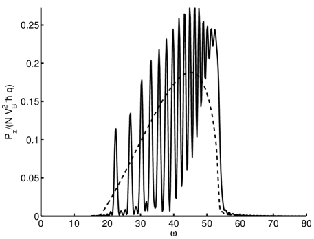
Figure 4: Same as in Fig. 2, but with $\eta=70$, $q=6\ a_{\rho}^{-1}$ and $t=6\ \omega_{\rho}^{-1}$.

The momentum transferred can also be calculated by direct integration of the time-dependent Gross-Pitaesvkii equation (1), using the definition (19) for $P_{z}$. In the linear response regime the results must concide with the ones of the quasiparticle projection method so far discussed. An example is shown in Fig. 5. The solid line corresponds to the momentum calculated with Eq. (21) at $t=6\omega_{\rho}^{-1}$, as in Fig. 2a. The empty squares are the results of GP simulations for a weak Bragg pulse ($V_{B}=10^{-3}\ \hbar\omega_{\rho}$). As expected, the two results are in good agreement, except for small differences that are compatible with the accuracy of our GP simulations. We also checked that, for such small values of $V_{B}$, the quantity $P_{z}(t)$ scales with $V_{B}^{2}$ as expected for the linear response.

A major advantage of using both approaches, is that one can now increase $V_{B}$, beyond the linear regime, and look at the differences between the linear response, given by Eq. (21), and the numerical GP calculation, which is valid also in the nonlinear regime bbg ; band . A typical result is shown in Fig. 5, where we compare the small $V_{B}$ limit (solid line and empty squares) with the results of GP simulations for $V_{B}=0.5\ \hbar\omega_{\rho}$ (solid circles). With such a pulse intensity, the fraction of condensate atoms which are excited is roughly $25\%$ at resonance. This value is slightly larger than that of typical experiments, where a fraction of the order of $10$-$20\%$ is required for the optical detection of the excited atoms. The figure shows that, even for such highly excited condensates, the main features of the multipeak response, associated with the underlying Bogoliubov spectrum, are still visible. The most significant effects of nonlinearity, originating from the mean-field interaction in the GP equation, are that i) $P_{z}$ does not scale with $V_{B}^{2}$, ii) the peak frequencies are slightly shifted downwards, and iii) additional structures appear superimposed to the original shape of the peaks. This behavior is a consequence of typical nonlinear processes like mode-mixing and higher harmonic generation. Similar effects were already predicted for spherical bbg and one-dimensional band condensates.

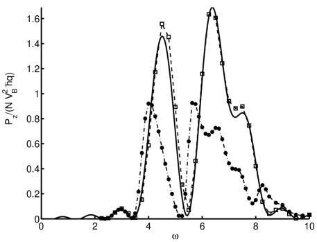
Figure 5: Momentum transferred to a cylindrical condensate with $\eta=9.4$ by a Bragg pulse with $q=2.3\ a_{\rho}^{-1}$. The quantity $P_{z}/(NV_{B}^{2}\hbar q)$, in units of $(\hbar\omega_{\rho})^{-2}$, is plotted vs. $\omega$, in units of $\omega_{\rho}$. The solid line corresponds to the result obtained from Eq. (21) at $t=6\ \omega_{\rho}^{-1}$ (same as in Fig. 2a). Empty squares and solid circles are the results of the numerical integration of the time dependent GP equation (1) for a Bragg pulse of intensity $V_{B}=10^{-3}\ \hbar\omega_{\rho}$ and $V_{B}=0.5\ \hbar\omega_{\rho}$, respectively. Dashed and dot-dashed lines are a guide to the eye.

V Bragg scattering from a prolate elongated condensate

Here we show that the main features found for the response of a cylindrical condensate to a Bragg pulse remain observable also in a finite elongated condensate.

Let us take the trapping potential in the form

$$V_{T}({\bf r})=(1/2)m\omega_{\rho}^{2}(\rho^{2}+\lambda^{2}z^{2})$$ (26)

where $\lambda=\omega_{z}/\omega_{\rho}$. If $\lambda<1$ the condensate at equilibrium is a prolate ellipsoid. The ground state at $t=0$ can be found as the stationary solution of Eq. (1). Then, the time dependent GP equation can be solved at $t>0$ to simulate the Bragg process.

In Figs. 6a and 6b we show typical results obtained for $P_{z}$ in the linear response (small $V_{B}$) regime. We simulate the Bragg scattering from two different condensates, whose chemical potential, in units of $\hbar\omega_{\rho}$, is equal to $9.4$ and $26.5$, as for the cylindrical condensates of Fig. 1 and 2. These two values correspond to the condensate used in the experiments of Ref. steinhauer2003 , made of $N=10^{5}$ atoms of ⁸⁷Rb in a trap with $\omega_{\perp}=2\pi(220$Hz$)$ and $\lambda=0.114$, and to the one used in the calculations of Refs. brunello ; brunello2 , with $\lambda=0.125$, respectively. With this choice, the condensates in Fig. 2a (2b) and 6a (6b) have also the same density profile in the radial direction for $z=0$. As one can see, the momentum transferred to the trapped condensates of Fig. 6 has the same multipeak structure of the corresponding cylindrical condensates of Fig. 2.

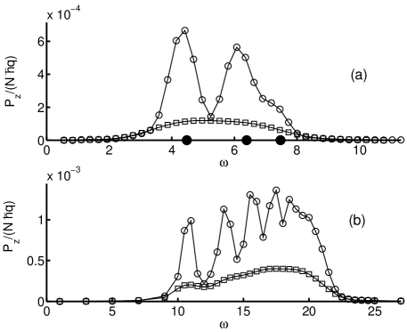
Figure 6: Momentum transferred to two different ellipsoidal condensates by a Bragg pulse. In part (a) the condensate has $\mu=9.4\hbar\omega_{\rho}$ and $\lambda=0.114$; the Bragg pulse has $q=2.3a_{\rho}^{-1}$ and $V_{B}=0.02\hbar\omega_{\rho}$. In part (b) the condensate has $\mu=26.5\hbar\omega_{\rho}$ and $\lambda=0.125$; the Bragg pulse has $q=4a_{\rho}^{-1}$ and $V_{B}=0.05\hbar\omega_{\rho}$. The points are obtained by numerically integrating the GP equation (1) for different $\omega$ (in units of $\omega_{\rho}$). The duration time is $t=2$ and $6\ \omega_{\rho}^{-1}$ for the lower and upper curves, respectively. The lines are a guide to the eye. The solid circles on the horizontal axis in (a) are the frequencies of the lowest Bogoliubov branches for that $q$.

The response of an ellipsoidal (axially confined) condensate is expected to differ from the one of a cylindrical (axially unbound) condensate for two main reasons. First, their Bogoliubov spectra are different: the excitations of a confined condensate are discretized also along $z$ and the quasiparticle amplitudes $u$ and $v$ have a nontrivial dependence on $\rho$ and $z$. Second, the response for long pulses is affected by the presence of the axial confinement, which can produce a reflection of quasiparticles at the boundaries and a center-of-mass motion of the condensate in the trap.

The first effect, however, is small if $q\gg L^{-1}$, where $L$ is the axial length of the condensate. In this case, the Bragg pulse excites quasiparticles that behave like travelling waves along $z$, having wavelength much shorter than the condensate size. One can safely introduce a continuous wavevector $k$ to identify such excitations as in the multibranch spectrum of the cylindrical condensate. The axial size of the two condensates in Figs. 6a and 6b is approximately $L=75$ and $120a_{\rho}$, respectively, so that the Bogoliubov modes can be safely represented by continuous branches down to about $k=0.5\ a_{\rho}^{-1}$. Moreover, for $k\gg L^{-1}$, the frequencies $\omega_{n,k}$ for the elongated ellipsoidal condensate are expected to be close to the ones of the corresponding cylindrical condensate, with a similar multibranch structure. In order to check that the peaks of $P_{z}$ are still located at the frequencies of the Bogoliubov branches, we make a further simulation for the condensate in Fig. 6a. We excite the condensate by acting with a Bragg pulse for a given duration $t$ and then we let it to freely evolve in the trap. We perform a Fourier analysis of the induced density variations in the axial direction. As expected, we find that, for each $q$ and $\omega$, the density oscillates as a superposition of waves of different frequencies $\omega_{n,k}$. The latter are extracted from the Fourier spectrum and reported in Fig. 6a as solid circles. As one can see, the momentum is resonantly transferred at those frequencies.

The second effect is also small if the duration time of the Bragg pulse is significantly less than the axial trapping period $T_{z}$. If $\lambda$ is of the order of $10^{-1}$, or less, there exists a sufficiently wide interval of time, between $T_{\rho}$ and $T_{z}$, where the multipeak structures of $P_{z}$ can be resolved without being significantly affected by the reflection of quasiparticles at the boundaries and by the center-of-mass motion.

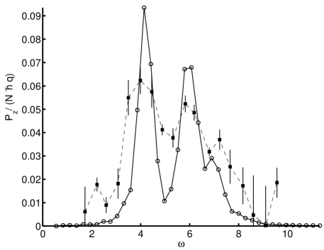
Figure 7: Momentum transferred to the condensates of Ref. steinhauer2003 . Empty symbols are obtained by numerically integrating the GP equation (1) for different values of $\omega$ (in units of $\omega_{\rho}$). Points with error bars are experimental data steinhauer2003 . The lines are a guide to the eye. The condensate is the same of Fig. 6a. The Bragg pulse has wavevector $q=2.3a_{\rho}^{-1}$, duration $t=6$ ms$=8.29\omega_{\rho}^{-1}$ and intensity $V_{B}=0.2\hbar\omega_{\rho}$.

Finally, the experimental observation of the excited atoms, requires rather high Bragg intensities. As already shown in the previous section, nonlinear processes are not expected to hinder the visibility of the multibranch Bogoliubov spectrum. Conversely, the combined use of both the quasiparticle projection method and the time dependent GP equation might allows one to extract from the observed $P_{z}$ information about nonlinear effects in the condensate dynamics.

In Fig. 7 the results of our GP simulations are compared with experimental measurements of $P_{z}$. Similar examples were already reported in Ref. steinhauer2003 , where the major sources of noise and broadening of the observed data were also discussed. The main message of Ref. steinhauer2003 was that the measured response to long Bragg pulses exhibits clear evidences of the underlying Bogoliubov spectrum. In the present paper we have provided a deeper theoretical analysis, which supports this view.

NUMERICAL PROCEDURES

• i) Stationary GP equation

  The ground state configuration at $t=0$ is obtained by solving the stationary GP equation (4) with the external potential given in (26). The case $\lambda=0$ corresponds to the cylindrical condensate of sections III and IV: the order parameter is uniform along $z$ and the problem is reduced to the one-dimensional equation (7). The solution of this equation is equivalent to the minimization of a GP energy functional rmp . We find the minimum by mapping the function $\phi_{0}$ on a grid of points and propagating it in imaginary time with an explicit first order algorithm, starting from a trial configuration, as described in Ref. ds . The case $\lambda\neq 0$ corresponds to an ellipsoidal condensate, as in section V. We use the same minimization algorithm. Due to the axial symmetry of $V_{T}$, the problem is two-dimensional. The order parameter is mapped on a $N_{\rho}\times N_{z}$ grid (typically, $64\times 1024$ points).

• ii) Time dependent GP equation

  Let us define an effective Hamiltonian $H$ by rewriting Eq. (1) in the form $i\hbar\partial_{t}\Psi=H\Psi$. We solve this equation by propagating the order parameter in real time, starting from the ground state configuration. At each time step, $\Delta t$, the evolution is determined by the implicit algorithm

  $$\left(1+\frac{i\Delta t}{2}H\right)\Psi_{n+1}=\left(1-\frac{i\Delta t}{2}H\right)\Psi_{n}$$ (27)

  where $H$ and $\Psi_{n}$ are calculated at the $n$-th iteration. For $\lambda\neq 0$, the propagation is splitted into the axial and radial parts. The former is obtained by using a fast Fourier transform algorithm to treat the kinetic energy term, while the latter is performed with a Crank-Nicholson differencing method, as in brunello . For the cylindrical case ($\lambda=0$), we first write the order parameter as $\Psi(\rho,z,t)=\sum_{\nu}\psi_{\nu}(\rho,t)\exp(i\nu qz)$, where $q$ is the wavevector of the Bragg potential, and then we propagate in time the radial functions $\phi_{\nu}$, for $\nu=0,\pm 1,\pm 2,\dots$. Only a few values of $\nu$ give significant contributions to the sum, their number depending on the intensity of the pulse.

• iii) Bogoliubov equations

  In order to solve the eigenvalue problem (9)-(10) for a cylindrical condensate, we project the unknown radial functions $u(\rho)$ and $v(\rho)$ on a basis set of Bessel functions. The problem is thus reduced to a matrix diagonalization. We use Bessel functions with up to 100 nodes in the computational box. The radius of the box is typically two or three times the size of the condensate.

References

- (1) J. Steinhauer, N.Katz, R. Ozeri, N. Davidson, C. Tozzo, and F. Dalfovo, Phys. Rev. Lett. 90, 060404 (2003).
- (2) S.A. Morgan, S. Choi, K. Burnett, and M. Edwards, Phys. Rev. A 57, 3818 (1998).
- (3) P.B. Blakie, R.J. Ballagh, and C.W. Gardiner, Phys. Rev. A 65, 033602 (2002).
- (4) J. Stenger, S. Inouye, A. P. Chikkatur, D. M. Stamper-Kurn, D. E. Pritchard, and W. Ketterle, Phys. Rev. Lett. 82, 4569 1999); D. M. Stamper-Kurn, A. P. Chikkatur, A. Görlitz, S. Inouye, S. Gupta, D. E. Pritchard, and W. Ketterle, Phys. Rev. Lett. 83, 2876 (1999); J. M. Vogels, K. Xu, C. Raman, J. R. Abo-Shaeer, and W. Ketterle, Phys. Rev. Lett. 88, 060402 (2002).
- (5) J. Steinhauer, R. Ozeri, N. Katz, and N. Davidson Phys. Rev. Lett. 88, 120407 (2002); R. Ozeri, J. Steinhauer, N. Katz, and N. Davidson, Phys. Rev. Lett. 88, 220401 (2002).
- (6) F. Dalfovo, S. Giorgini, L. Pitaevskii and S. Stringari, Rev. Mod. Phys. 71, 463 (1999).
- (7) N. N. Bogoliubov, J. Phys. (USSR) 11, 23 (1947).
- (8) L.P. Pitaevskii, Zh. Eksp. Teor. Fiz. 40, 646 (1961) [Sov. Phys. JETP 13, 451 (1961)].
- (9) A.L. Fetter, Ann. Phys. (N.Y.) 70, 67 (1972).
- (10) Other solutions are complex functions associated with the occurrence of stationary currents, as in the case of quantized vortices. The application of GP theory to Bragg scattering from condensates with vortices has been discussed in P.B. Blakie and R.J. Ballagh, Phys. Rev. Lett. 86, 3930 (2001), and in Ref. bbg .
- (11) P.O. Fedichev and G.V. Shlyapnikov, Phys. Rev. A 63, 045601 (2001).
- (12) M. Guilleumas and L. Pitaesvkii, e-print cond-mat/0208047.
- (13) S. Komineas and N. Papanicolaou, Phys. Rev. A 67, 023615 (2003).
- (14) In this context, the Thomas-Fermi approximation corresponds to neglecting the quantum pressure term, , in the stationary GP equation (7). The density takes the form of an inverted parabola and the chemical potential can be easily calculated from the normalization.
- (15) R. Onofrio, C. Raman, J. M. Vogels, J. R. Abo-Shaeer, A. P. Chikkatur, and W. Ketterle, Phys. Rev. Lett. 85, 2228 (2000).
- (16) A. Brunello, F. Dalfovo, L. Pitaevskii, S. Stringari, and F. Zambelli, Phys. Rev. A 64, 063614 (2001).
- (17) A. Brunello, F. Dalfovo, L. Pitaevskii, and S. Stringari, Phys. Rev. Lett. 85, 4422 (2000).
- (18) L.P. Pitaevskii and A. Rosch, Phys. Rev. A 55, R853 (1997); F. Chevy, V. Bretin, P. Rosenbusch, K. W. Madison, and J. Dalibard, Phys. Rev. Lett. 88, 250402 (2002).
- (19) P. Öhberg, E.L. Surkov, I. Tittonen, S. Stenholm, M. Wilkens, and G.V. Shlyapnikov, Phys. Rev. A 56, R3346 (1997); S. Stringari, Phys. Rev. A 58, 2385 (1998); E. Zaremba, Phys. Rev. A 57, 518 (1998).
- (20) P. B. Blakie and R. J. Ballagh, J. Phys. B 33, 3961 (2000).
- (21) A. Csordás, R. Graham, and P. Szépfalusy, Phys. Rev. A 54, R2543 (1196).
- (22) F. Zambelli, L. Pitaevskii, D.M. Stamper-Kurn, and S. Stringari, Phys. Rev. A 61, 063608 (2000).
- (23) Y.B. Band and M. Sokuler, Phys. Rev. A 66, 043614 (2002).
- (24) F. Dalfovo and S. Stringari, Phys. Rev. A 53, 2477, (1996).