Transport properties of correlated electrons in high dimensions

Abstract

We develop a new general algorithm for finding a regular tight-binding lattice Hamiltonian in infinite dimensions for an arbitrary given shape of the density of states (DOS). The availability of such an algorithm is essential for the investigation of broken-symmetry phases of interacting electron systems and for the computation of transport properties within the dynamical mean-field theory (DMFT). The algorithm enables us to calculate the optical conductivity fully consistently on a regular lattice, e.g., for the semi-elliptical (Bethe) DOS. We discuss the relevant $f$-sum rule and present numerical results obtained using quantum Monte Carlo techniques.

1 Introduction

Microscopic studies of strongly correlated electron systems require methods which take the Coulomb repulsion between electrons explicitly into account. Many features of such systems can be modeled using the single-band Hubbard model [1]

$$\hat{H}=\hat{H}_{0}+\hat{H}_{\text{int}}=\sum_{ij,\sigma}t_{ij}\;\hat{c}_{{\bm{R}}_{i}\sigma}^{\dagger}\hat{c}_{{\bm{R}}_{j}\sigma}^{{\phantom{\dagger}}}+U\sum_{i}\hat{n}_{{\bm{R}}_{i}\uparrow}\hat{n}_{{\bm{R}}_{i}\downarrow}\,,$$ (1)

where the operators $\hat{c}_{{\bm{R}}_{i}\sigma}^{\dagger}$ and $\hat{c}_{{\bm{R}}_{i}\sigma}^{\phantom{\dagger}}$ create and destroy electrons of spin $\sigma$ on site ${\bm{R}}_{i}$, respectively; $\hat{n}_{{\bm{R}}_{i}\sigma}$ measures the corresponding occupancy. A general nonperturbative treatment of this model is only possible in the limit of infinite dimensionality where the dynamical mean-field theory becomes exact: due to a local self-energy the model reduces for $d\to\infty$ to a single impurity Anderson model plus a self-consistency equation. For homogeneous phases, local properties then only depend on the lattice via the noninteracting DOS $\rho(\epsilon):=\frac{1}{N}\sum_{\bm{k}}\delta(\epsilon-\epsilon_{\bm{k}})$. In the simplest case of uniform nearest-neighbor hopping on a hypercubic (hc) lattice, the dispersion reads $\epsilon_{\bm{k}}^{\text{hc}}=-2t\sum_{\alpha=1}^{d}\cos(k_{\alpha})$ which for the proper scaling $t=t^{*}/\sqrt{2d}$ leads to a Gaussian DOS $\rho^{\text{hc}}(\epsilon)=\exp[-\epsilon^{2}/(2{t^{*}}^{2})]/(\sqrt{2\pi}t^{*})$.

Vertex corrections to the optical conductivity $\sigma(\omega)$ vanish [2] in the limit $d\to\infty$ so that it may be expressed in the isotropic case as [3]

$$\sigma(\omega)=\sigma_{0}\!\int_{-\infty}^{\infty}\!\!\mathrm{d}\epsilon\,\tilde{\rho}(\epsilon)\int_{-\infty}^{\infty}\!\!\mathrm{d}\omega^{\prime}\,A_{\epsilon}(\omega^{\prime})A_{\epsilon}(\omega^{\prime}+\omega)\frac{n_{\text{f}}(\omega^{\prime})-n_{\text{f}}(\omega+\omega^{\prime})}{\omega}\,.$$ (2)

Here, $A_{\epsilon}(\omega)$ is the “momentum” dependent spectral function, $n_{\text{f}}(\omega^{\prime})$ is the Fermi function, $\sigma_{0}=\frac{2\pi e^{2}}{\hbar^{2}}\frac{N}{V}$, and

$$\tilde{\rho}(\epsilon):=\frac{1}{N}\sum_{\bm{k}}|{\bm{v}}_{{\bm{k}}}|^{2}\delta(\epsilon-\epsilon_{\bm{k}})=:\langle|{\bm{v}}_{{\bm{k}}}|^{2}\rangle(\epsilon)\,\rho(\epsilon)\,.$$ (3)

Note that the frequency- and interaction-dependent part in (2) depends on the lattice only via the DOS while the explicitly lattice-dependent part $\tilde{\rho}(\epsilon)$ is universal, i.e., independent of interaction $U$, filling, and temperature. In the hypercubic case, the momentum dependence of the Fermi velocity ${\bm{v}}_{{\bm{k}}}$ becomes irrelevant in (3) for $d\to\infty$; for unit hopping and lattice spacing, one observes $\tilde{\rho}^{\text{hc}}(\epsilon)=\rho^{\text{hc}}(\epsilon)$. As a consequence, the optical $f$-sum is then proportional to the kinetic energy:

$$\int_{0}^{\infty}\!\mathrm{d}\omega\,\sigma(\omega)=-\frac{\sigma_{0}}{4}\langle\hat{H_{0}}\rangle\,.$$ (4)

However, the hc DOS is unbounded which is hardly compatible with the single-band assumption. In fact, no regular lattice model with sharp band edges in $d\to\infty$ could be constructed so far. In this situation, many DMFT studies have focussed on the so-called Bethe lattice which is not a regular lattice, but a tree in the sense of graph theory as shown in Fig. 1a.

a)                                          b)                                      c)

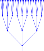
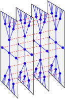
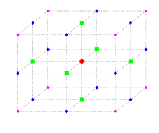
Figure 1: Bethe lattice: a) conventional tree level picture for coordination $Z=4$, b) stacked Bethe lattice, c) redefined Bethe lattice as a regular lattice with cubic symmetry: here, symbols denote equal hopping matrix elements relative to a fixed site (central circle).

The semi-elliptic DOS $\rho(\epsilon)=\sqrt{4-\epsilon^{2}}/(2\pi)$ of this model (for $Z\to\infty$) fixes the local properties of the model; transport, however, is a priori undefined. A derivation of $\sigma(\omega)$ directly for the Bethe tree (using the level-picture Fig. 1a) by Chung and Freericks [4] is still incomplete [5]; up to a factor of 3, the same expression $\tilde{\rho}(\epsilon)\propto(4-\epsilon^{2})\rho(\epsilon)$ was obtained [6] in a heuristic scheme by enforcing the hc $f$-sum rule (4). An alternative direct approach [7] fails to describe the coherent transport expected in the metallic regime.

The local DMFT problem is unchanged when a finite number of hopping bonds per site are added. Therefore, the periodically stacked Bethe lattice (Fig. 1b) is still a Bethe lattice in the DMFT sense; potentially coherent transport is then well-defined (only) in stacking direction [8]. A semi-elliptic DOS also results from fully disordered hopping on lattices of arbitrary topology; in this case, $\sigma(\omega)$ is incoherent [9].

We will in the following construct and evaluate a new definition for $\sigma(\omega)$ compatible with a semi-elliptic DOS. This definition is unique by being based on a regular lattice as illustrated in Fig. 1c and by leading to an isotropic conductivity which is coherent in the noninteracting limit.

2 General Dispersion Method

We rewrite the translation-invariant noninteracting Hamiltonian,

$$\hat{H}_{0}=\sum_{i,\sigma}\sum_{\bm{\tau}}t_{\bm{\tau}}\;\hat{c}_{{\bm{R}}_{i}\sigma}^{\dagger}\hat{c}_{{\bm{R}}_{i}+{\bm{\tau}},\sigma}^{{\phantom{\dagger}}}=\sum_{{\bm{k}},\sigma}\epsilon({\bm{k}})\,\hat{n}_{{\bm{k}}\sigma},$$ (5)

where contributions to the dispersion may be classified by the taxi-cab hopping distance $|\>\!\!|\bm{\tau}|\>\!\!|=\sum_{\alpha=1}^{d}|\tau_{\alpha}|$:

$$\epsilon({\bm{k}})=\sum_{D=1}^{\infty}\epsilon_{D}({\bm{k}}),\qquad\epsilon_{D}({\bm{k}})=\sum_{|\>\!\!|\bm{\tau}|\>\!\!|=D}t_{\bm{\tau}}e^{i{\bm{\tau}}\cdot{\bm{k}}}\,.$$ (6)

In high dimensions, only vectors of the form ${\bm{\tau}}=\sum_{i=1}^{D}{\bm{e}}_{\alpha_{i}}$ with pairwise different directions $\alpha_{i}$ need to be considered. This follows from the fact that the fraction of neglected vectors (with $|{\bm{\tau}}\cdot{\bm{e}}_{\alpha}|>1$ for some direction $\alpha$) vanishes as $1/d$. Furthermore, the considered vectors are of minimal Euclidean length $|{\bm{\tau}}|$ hinting at maximal overlap, i.e., largest $|t_{\bm{\tau}}|$ for fixed taxi-cab distance $|\>\!\!|\bm{\tau}|\>\!\!|$ and fixed $D$.

By deriving a recursion relation for $\epsilon_{D}({\bm{k}})$ we have established that

$$\epsilon({\bm{k}})\,=\,\sum_{D=1}^{\infty}\frac{t_{D}^{*}}{\sqrt{D!}}\;\text{He}_{D}(\epsilon^{\text{hc}}_{\bm{k}})\,=:\,{\cal F}(\epsilon^{\text{hc}}_{\bm{k}})\,.$$ (7)

Using the orthogonality of the Hermite polynomials, one may express the hopping matrix elements in terms of the transformation function ${\cal F}(x)$:

$$t_{D}^{*}=\frac{1}{\sqrt{2\pi D!}}\int_{-\infty}^{\infty}\!\mathrm{d}\epsilon\,{\cal F}(\epsilon)\,\text{He}_{D}(\epsilon)\,e^{-\epsilon^{2}/2}\,.$$ (8)

Specializing on the case of a monotonic transformation function ${\cal F}(x)$ (with derivative ${\cal F}^{\prime}(x)$), we can write

$$\rho(\epsilon)=\frac{1}{{\cal F}^{\prime}({\cal F}^{-1}(\epsilon))}\,\rho^{\text{hc}}({\cal F}^{-1}(\epsilon))$$ (9)

which leads to

$${\cal F}^{-1}(\epsilon)=\sqrt{2}\;\text{erf}^{-1}\bigg{(}2\int_{-\infty}^{\epsilon}\!\mathrm{d}\epsilon^{\prime}\rho(\epsilon^{\prime})-1\bigg{)}\,.$$ (10)

Furthermore, the Fermi velocity ${\bm{v}}_{\bm{k}}=\nabla\epsilon_{\bm{k}}$ can be computed:

$${\bm{v}}_{\bm{k}}={\cal F}^{\prime}({\cal F}^{-1}(\epsilon)){\bm{v}}_{\bm{k}}^{\text{hc}}=\frac{\rho^{\text{hc}}(\sqrt{2}\,\text{erf}^{-1}(2\int_{-\infty}^{\epsilon}\!\mathrm{d}\epsilon^{\prime}\rho(\epsilon^{\prime})-1))}{\rho(\epsilon)}\,{\bm{v}}_{\bm{k}}^{\text{hc}}\,.$$ (11)

A practical application of the general formalism proceeds as follows:

1. compute ${\cal F}^{-1}(\epsilon)$ from arbitrary target DOS $\rho(\epsilon)$ using (10)

2. invert function (numerically or analytically) to obtain ${\cal F}(\epsilon)$

3. evaluate transport properties, e.g., $\langle|{\bm{v}}_{\bm{k}}|^{2}\rangle(\epsilon)$ or $\tilde{\rho}(\epsilon)$ using (11)

4. optionally determine microscopic model parameters $t_{D}^{*}$ using (8)

The only choice inherent in this procedure beyond the usual assumptions for large dimensions is contained in step 1 which by construction produces a monotonic transformation function ${\cal F}$. The optical $f$-sum rule reads

$$\int_{0}^{\infty}\!\mathrm{d}\omega\,\sigma_{xx}(\omega)=\displaystyle\frac{\sigma_{0}}{4d}\,\big{\langle}\frac{\tilde{\rho}^{\prime}(\epsilon)}{\rho(\epsilon)}\big{\rangle}=\displaystyle\frac{\sigma_{0}}{4d}\,\left\langle\left[{\cal F}^{\prime\prime}\big{(}{\cal F}^{-1}(\epsilon)\big{)}-{\cal F}^{-1}(\epsilon){\cal F}^{\prime}\big{(}{\cal F}^{-1}(\epsilon)\big{)}\right]\right\rangle\,.$$ (12)

Here, the first equality follows from (2), i.e., is generally valid within the DMFT while the second expression in terms of the transformation is specific to the formalism developed within this section.

Example: Flat-band System

One interesting limiting case of a monotonic transformation function which can be treated analytically is the step function ${\cal F}(x)=2\Theta(x)\!-\!1$ corresponding to a flat band DOS of the form $\rho(\epsilon)=\big{(}\delta(\epsilon\!-\!1)+\delta(\epsilon\!+\!1)\big{)}/2$. For this case, the hopping matrix elements read (trivially, $t_{2n}^{*}=0$):

$$t_{2n+1}^{*}=(-1)^{n}\sqrt{\frac{2}{\pi}}\frac{(2n-1)!!}{\sqrt{(2n+1)!}}\quad\stackrel{{\scriptstyle n\to\infty}}{{\longrightarrow}}\quad(-1)^{n}(\pi n)^{-3/4}\;.$$ (13)

The asymptotic exponent $-3/4$ is only slightly smaller than the threshold value $-1/2$ required for a finite variance $\int_{-\infty}^{\infty}d\epsilon\,\epsilon^{2}\rho(\epsilon)=\sum_{D}{t_{D}^{*}}^{2}$. For a rectangular model DOS, $t_{D}^{*}\sim 2^{-n}n^{-3/4}$ already decays exponentially fast.

3 Application to the “Bethe” semi-elliptic DOS

In this section, we will apply the new formalism to the Bethe semi-elliptic DOS in order to determine a corresponding tight-binding Hamiltonian defined on the hypercubic lattice with the same local properties as the Bethe lattice (with NN hopping) in the limit $d\to\infty$. From (11), we derive the average squared Fermi velocity defined in (3) in closed form:

$$\langle|{\bm{v}}_{\bm{k}}|^{2}\rangle(\epsilon)=\frac{2\pi}{4-\epsilon^{2}}\exp\left[-2\left(\!\text{erf}^{-1}\Big{(}\frac{\epsilon\sqrt{1-\epsilon^{2}/4}+2\arcsin(\epsilon/2)}{\pi}\Big{)}\!\!\right)^{\!\!2}\right]\,.$$ (14)

Here, we have used the fact that $\langle|{\bm{v}}_{\bm{k}}|^{2}\rangle(\epsilon)$ is effectively constant (and equals 1 for unit variance and lattice spacing) in the hypercubic case. The result (solid line in Fig. 2a)

a)                                                                b)

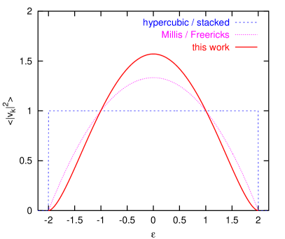
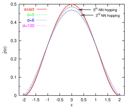
Figure 2: a) The average squared Fermi velocity $\langle|{\bm{v}}_{\bm{k}}|^{2}\rangle(\epsilon)$ is constant for the hypercubic lattice (or for the $x$-component of a stacked lattice); in contrast it vanishes for the isotropic lattice defined in this work. For comparison, the form suggested by Millis is also shown. b) Resulting function $\tilde{\rho}(\epsilon)$ of the full isotropic model (solid line) in comparison with truncated models ($D_{\max}=3$ or $D_{\max}=5$), evaluated in finite dimensions $5\leq d\leq 100$.

has all the qualitative features expected for this observable in any finite dimension: $\langle|{\bm{v}}_{\bm{k}}|^{2}\rangle(\epsilon)$ is maximal near the band center, strongly reduced for large (absolute) energies and vanishes at the band edges: states at a (noninteracting) band edge do not contribute to transport. The violation of this principle in the stacked case (dashed lines in Fig. 2a), which corresponds to an application of the hc formalism to the Bethe DOS with $\langle|{\bm{v}}_{\bm{k}}|^{2}\rangle$ constant up to the band edges, is clearly pathological. Therefore, our method has not only the merit of yielding isotropic transport, but also of avoiding unphysical behavior.

In order to determine the microscopic model, we have to apply (8) to the numerically evaluated transformation function ${\cal F}$. Again, the scaled hopping matrix elements fall off exponentially fast: only a fraction $10^{-3}$ of the total energy variance arises from hopping amplitudes beyond third nearest neighbors and only a fraction $10^{-6}$ results from hopping beyond $9^{\text{th}}$-nearest neighbors. This result suggests that properties of the model should be robust with respect to truncation. In fact, $\tilde{\rho}(\epsilon)$ (and consequently the definition of $\sigma(\omega)$) hardly changes when hopping is cut off beyond $3^{\text{rd}}$ or $5^{\text{th}}$ nearest neighbors, even when evaluated in finite dimensions as seen in Fig. 2b. This behavior is very general so that results for $\sigma(\omega)$ of a local theory in finite dimensions will depend on $d$ predominantly via the interacting DOS $A(\omega)$ and only very little via $\tilde{\rho}(\epsilon)$.

The local spectral functions for $T=0.05$, i.e., slightly below the critical temperature $T^{*}\approx 0.055$, are shown in Fig. 3a as obtained from QMC/MEM [5]. In the metallic phase, the spectral density at the Fermi level ($\omega=0$) is approximately pinned at the noninteracting value $\rho(0)=1/\pi\approx 0.32$ for $U\lesssim 4.4$. The quasiparticle weight decreases drastically and a shoulder develops for $U\gtrsim 4.6$ before a gap opens for $U\gtrsim 4.8$. An application of (2) to these spectra for the isotropic model characterized by (14) yields the estimates for the optical conductivity $\sigma(\omega)$ shown in Fig. 3b.

a)                                                                b)

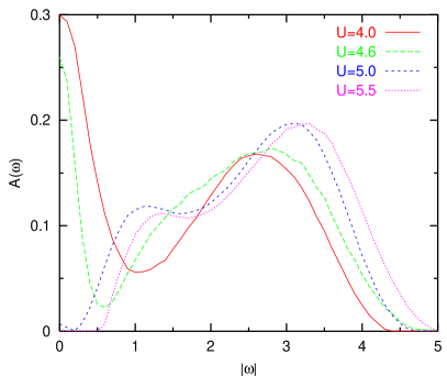
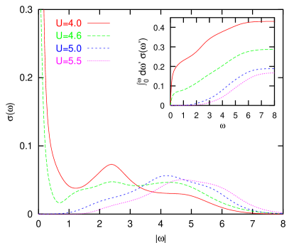
Figure 3: Numerical results for the half-filled Hubbard model with semi-elliptic DOS for $d\to\infty$ in the paramagnetic phase at $T=0.05$. a) Local spectral function $A(\omega)$ obtained from QMC (using a discretization $\Delta\tau=0.1$) and MEM. b) Optical conductivity $\sigma(\omega)$ for the isotropic “redefined Bethe lattice”. The inset shows the partial $f$-sum $\int_{0}^{\omega}\!\mathrm{d}\omega^{\prime}\sigma(\omega^{\prime})$.

A low-frequency Drude peak (of Lorentzian form) and a mid-infrared peak at $\omega\approx U/2$ are present in the metallic phase and decay towards the metal-insulator transition at $U\approx 4.7$. For large $U$, the optical spectral weight concentrates in incoherent peaks at $\omega\approx U$. The inset of Fig. 3b shows the partial optical $f$-sums. As expected, both the contribution of the Drude peak and the total $f$-sum decrease for increasing $U$.

Figure 4a shows the impact of the definition for $\sigma(\omega)$ on the results for $U=4.0$. Our isotropic model yields by far the largest contributions at small $\omega$. While the stacked model leads to otherwise similar results, the low-frequency form of $\sigma(\omega)$ is qualitatively different in the disordered case (where a Drude peak is absent even for $U\to 0$). As seen in Fig. 4b,

a)                                                                b)

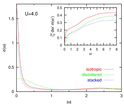
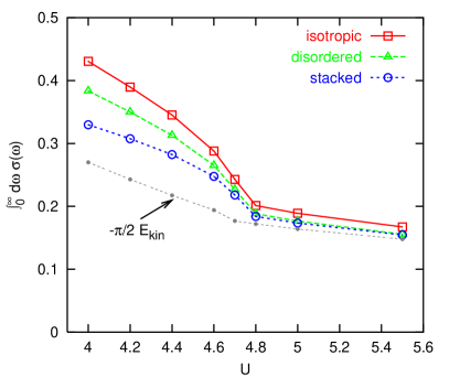
Figure 4: a) Optical conductivity $\sigma(\omega)$ for $T=0.05$ and $U=4.0$ for the new isotropic model with semi-elliptic DOS in comparison with disordered and stacked models consistent with the same DOS. b) Optical $f$-sum for $T=0.05$.

the $f$-sum is generally larger for the isotropic than for the stacked Bethe lattice, in particular in the metallic phase (while the disordered case is in-between). These differences can be attributed to the enhanced squared Fermi velocity in the isotropic model: The enhancement is largest near the Fermi surface, at $\epsilon=0$ by a factor of $\pi/2\approx 1.57$. A corresponding increase is expected of the Drude peak for small enough $U$ and $T$ when transport is dominated by states with $\epsilon\approx 0$. Since energy eigenstates spread out in momentum space at large $U$, the enhancement reduces (in general) to the integral $\int_{-\infty}^{\infty}\!\mathrm{d}\epsilon\,\tilde{\rho}(\epsilon)=\sum_{D=1}^{\infty}D\,{t_{D}^{*}}^{2}$ which evaluates here to 1.05406.

In all three cases, the proportionality (4) of the $f$-sum to the kinetic energy as characteristic for the hc lattice is clearly violated. This is true even for the stacked case (which is otherwise similar to the hc case): while the $f$-sum is here proportional to the contribution to the kinetic energy associated with hopping in current direction [8], $\int_{0}^{\infty}\!\mathrm{d}\omega\,\sigma_{xx}(\omega)=-\sigma_{0}\langle\hat{T}_{x}\rangle/4$, this contribution (which is negligible in the limit $Z\to\infty$) is not proportional to the total kinetic energy in this anisotropic case. A more relevant sum rule is derived from (12): $\int_{0}^{\infty}\!\mathrm{d}\omega\,\sigma_{xx}(\omega)=\frac{t^{2}a^{2}\sigma_{0}}{4}\langle\frac{-\epsilon}{4-\epsilon^{2}}\rangle$.

4 Conclusion

We have presented a new general method for constructing regular lattice models with hypercubic (hc) symmetry, i.e. isotropic optical transport properties, in large dimensions. Previously, calculations of the optical conductivity $\sigma(\omega)$ of the Hubbard model in the limit $d\to\infty$ had been restricted to the hypercubic lattice (using NCA [3] or QMC [10]) or have ignored the lattice dependence: Applying the hc formalism to the Bethe semi-elliptic DOS, Rozenberg et. al [11] overlooked violations of the hc $f$-sum rule. All previous approaches specific to the Bethe DOS were associated with anisotropic or incoherent transport; the most interesting of these [4, 6] have not yet been linked rigorously to microscopic models.

Our method yields the first derivation for $\sigma(\omega)$ consistent with a semi-elliptic DOS that implies isotropic transport which is fully coherent in the noninteracting limit. This reinterpretation of the “Bethe lattice” (in the DMFT sense) as an isotropic, regular and clean lattice and the demonstration that the associated transport properties are robust (with respect to finite dimensionality or hopping range) removes, finally, the pathologies previously associated with the DMFT treatment of transport in connection with non-Gaussian DOSs. At essentially no additional cost, the method can also be used for computing properties such as transverse conductivities and thermopower; these vanish, however, in the particle-hole symmetric case considered in this paper. Our numerical results have shown that the precise definition of $\sigma(\omega)$ does matter, in particular within the metallic phase where transport is potentially most coherent. We have also found a general DMFT expression for the $f$-sum rule as well as a form specific to our new approach.

- [1] J. Hubbard, Proc. Roy. Soc. London A276, 238 (1963). M. C. Gutzwiller, Phys. Rev. Lett. 10, 59 (1963). J. Kanamori, Prog. Theor. Phys. 30, 275 (1963).
- [2] A. Khurana, Phys. Rev. Lett. 64, 1990 (1990).
- [3] T. Pruschke, D. L. Cox, and M. Jarrell, Phys. Rev. B 47, 3553 (1993).
- [4] W. Chung and J. K. Freericks, Phys. Rev. B 57, 11955 (1998). J. K. Freericks, private communication (2000, 2002).
- [5] N. Blümer, Ph.D. Thesis, Universität Augsburg, 2002.
- [6] A. Chattopadhyay, A. J. Millis, and S. Das Sarma, Phys. Rev. B 61, 10738 (2000). A. J. Millis, private communication (2002).
- [7] M. P. H. Stumpf, Ph.D. Thesis, University of Oxford (1999).
- [8] G. S. Uhrig and R. Vlaming, J. Phys. Cond. Matter 5, 2561 (1993).
- [9] V. Dobrosavljević and G. Kotliar, Phys. Rev. Lett. 71, 3218 (1993).
- [10] M. Jarrell, J. K. Freericks, and T. Pruschke, Phys. Rev. B 51, 11704 (1995).
- [11] M. J. Rozenberg et. al, Phys. Rev. Lett. 75, 105 (1995).