Properties of highly clustered networks

Abstract

We propose and solve exactly a model of a network that has both a tunable degree distribution and a tunable clustering coefficient. Among other things, our results indicate that increased clustering leads to a decrease in the size of the giant component of the network. We also study SIR-type epidemic processes within the model and find that clustering decreases the size of epidemics, but also decreases the epidemic threshold, making it easier for diseases to spread. In addition, clustering causes epidemics to saturate sooner, meaning that they infect a near-maximal fraction of the network for quite low transmission rates.

I Introduction

There has in recent years been considerable interest within the physics community in the structure and dynamics of networks, with applications to the Internet, the World-Wide Web, citation networks, and social and biological networks Strogatz01 ; AB02 ; DM02 . Two significant properties of networks have been particularly highlighted. First, one observes for most networks that the degree distribution is highly non-Poissonian AJB99 ; FFF99 ; ASBS00 ; Newman01a ; Liljeros01 . (A network consists of a set of nodes or “vertices”, joined by lines or “edges”, and the degree of a vertex is the number of edges attached to that vertex.) Histograms of vertex degree for many networks show a power-law form with exponent typically between $-2$ and $-3$, while other networks may have exponential or truncated power-law distributions. Second, it is found that most networks have a high degree of transitivity or clustering, i.e., that there is a high probability that “the friend of my friend is also my friend” WS98 . In topological terms, this means that there is a heightened density of loops of length three in the network, and more generally it is found that networks have a heightened density of short loops of various lengths CPV03 .

It is now well understood how to calculate the properties of networks with arbitrary degree distributions MR95 ; MR98 ; ACL00 ; NSW01 ; CL02a , but where clustering is concerned our understanding is much poorer. Most of the standard techniques used to solve network models break down when clustering is introduced, obliging researchers to turn to numerical methods WS98 ; KE02 ; HK02b ; MV03 .

In this paper, we present a plausible network model that incorporates both non-Poisson degree distributions and non-trivial clustering, and which is exactly solvable for many of its properties, including component sizes, percolation threshold, and clustering coefficient. Our results show that clustering can have a substantial effect on the large-scale structure of networks, and produces behaviors that are both quantitatively and qualitatively different from the simple non-clustered case.

The outline of the paper is as follows. In Sec. II we define our model and in Sec. III we derive exact expressions for a variety of its properties. In Sec. IV we discuss the form of these expressions for some sensible choices of the parameters, and also consider the behavior of epidemic processes within our model. In Sec. V we give our conclusions.

II The model

There is empirical evidence that clustering in networks arises because the vertices are divided into groups DGM02a ; RB03 , with a high density of edges between members of the same group, and hence a high density of triangles, even though the density of edges in the network as a whole may be low. Our model is perhaps the simplest and most obvious realization of this idea. We describe it here in the anthropomorphic language of social networks, although our arguments apply equally to non-social networks.

We consider a network of $N$ individuals divided into $M$ groups. A social network, for example, might be divided up according to the location, interests, occupation, and so forth of its members. (Many networks are indeed known to be divided into such groups GN02 .) Individuals can belong to more than one group, the groups they belong to being chosen—in our model—at random. Individuals are not necessarily acquainted with all other members of their groups. If two individuals belong to the same group then there is a probability $p$ that they are acquainted and $q=1-p$ that they are not; if they have no groups in common then they are not acquainted. (A more sophisticated model in which there are many nested levels of groups within groups and a spectrum of acquaintance probabilities depending on these levels has been proposed and studied numerically by Watts et al. WDN02 . For this paper, however, we confine ourselves to the simpler case.) In addition to the probability $p$, the model is parametrized by two probability distributions: $r_{m}$ is the probability that an individual belongs to $m$ groups and $s_{n}$ is the probability that a group contains $n$ individuals.

Mathematically, the model can be regarded as a bond percolation model on the one-mode projection of a bipartite random graph. The structure of individuals and groups forms the bipartite graph, the network of shared groups is the projection of that graph onto the individuals alone, and the probability $p$ that one of the possible contacts in this projection is actually realized corresponds to a bond percolation process on the projection. See Fig. 1.

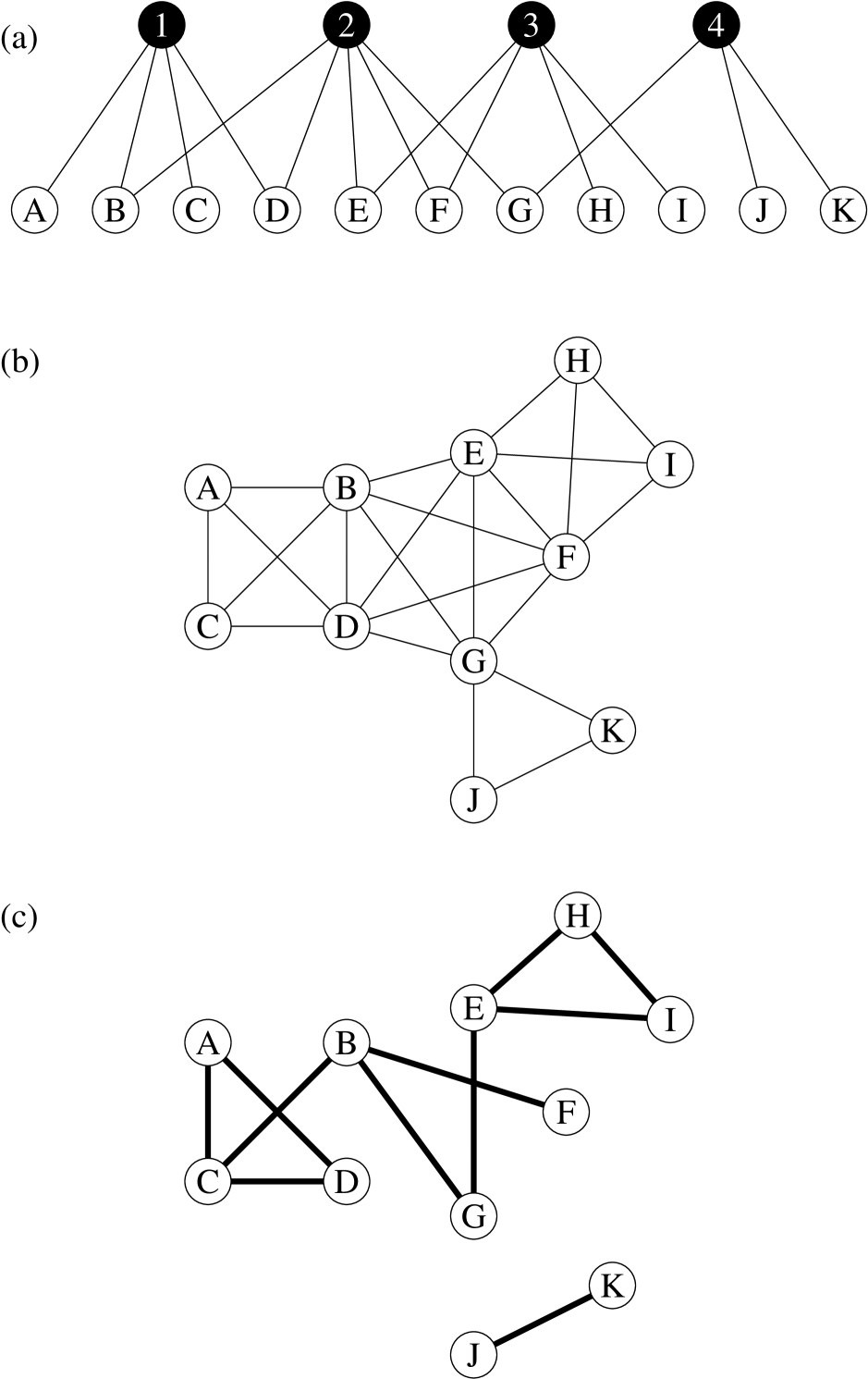
Figure 1: The structure of the network model described in this paper. (a) We represent individuals (A–K) and the groups (1–4) to which they belong with a bipartite graph structure. (b) The bipartite graph is projected onto the individuals only. (c) The connections between individuals are chosen by bond percolation on this projection with bond occupation probability $p$. The net result is that individuals have probability $p$ of knowing others with whom they share a group.

III Analytic developments

We can derive a variety of exact results for our model in the limit of large size using generating function methods. There are four fundamental generating functions that we will use:

$$\!\!f_{0}(z) = \!\sum_{m=0}^{\infty}r_{m}z^{m},\hskip 8.0ptf_{1}(z)=\mu^{-1}\sum_{m=0}^{\infty}mr_{m}z^{m-1},$$ (1)

$$\!\!g_{0}(z) = \sum_{n=0}^{\infty}s_{n}z^{n},\hskip 12.2ptg_{1}(z)=\nu^{-1}\sum_{n=0}^{\infty}ns_{n}z^{n-1},$$ (2)

where $\mu=\sum_{m}mr_{m}$ and $\nu=\sum_{n}ns_{n}$ are the mean numbers of groups per person and people per group respectively.

III.1 Degree distribution

Consider a randomly chosen person A, who belongs to some number of groups $m$. The number $j$ of A’s acquaintances within one particular group of size $n$ is binomially distributed according to ${n-1\choose j}p^{j}q^{n-1-j}$. We represent this distribution by its generating function:

$$\sum_{j=0}^{n-1}{n-1\choose j}p^{j}q^{n-1-j}z^{j}=[pz+q]^{n-1}.$$ (3)

Averaging over group size, the full generating function for neighbors in a single group is $\nu^{-1}\sum_{n=0}^{\infty}ns_{n}[pz+q]^{n-1}=g_{1}(pz+q)$, and for neighbors of a single person is $f_{0}(g_{1}(pz+q))$. This allows us to calculate the degree distribution for any given $\{r_{m},s_{n}\}$, and by judicious choice of the fundamental distributions, we can arrange for the degree distribution to take a wide variety of forms. We give some examples shortly. The mean degree $\langle k\rangle$ of an individual in the network is given by

$$\langle k\rangle=\bigl{[}{\partial_{z}}f_{0}(g_{1}(pz+q))\bigr{]}_{z=1}\!\!=p\mu g_{1}^{\prime}(1).$$ (4)

$k$	$P(k|k)$
1	$1$
2	$p$
3	$3\,p^{2}q+p^{3}$
4	$16\,p^{3}q^{3}+15\,p^{4}q^{2}+6\,p^{5}q+p^{6}$
5	$125\,p^{4}q^{6}+222\,p^{5}q^{5}+205\,p^{6}q^{4}+120\,p^{7}q^{3}+45\,p^{8}q^{2}+10\,p^{9}q+p^{10}$
6	$1296\,p^{5}q^{10}+3660\,p^{6}q^{9}+5700\,p^{7}q^{8}+6165\,p^{8}q^{7}+4945\,p^{9}q^{6}+2997\,p^{10}q^{5}+1365\,p^{11}q^{4}+455\,p^{12}q^{3}+105\,p^{13}q^{2}$
	${}+15\,p^{14}q+p^{15}$
7	$16807\,p^{6}q^{15}+68295\,p^{7}q^{14}+156555\,p^{8}q^{13}+258125\,p^{9}q^{12}+331506\,p^{10}q^{11}+343140\,p^{11}q^{10}+290745\,p^{12}q^{9}$
	${}+202755\,p^{13}q^{8}+116175\,p^{14}q^{7}+54257\,p^{15}q^{6}+20349\,p^{16}q^{5}+5985\,p^{17}q^{4}+1330\,p^{18}q^{3}+210\,p^{19}q^{2}+21\,p^{20}q+p^{21}$
8	$262144\,p^{7}q^{21}+1436568\,p^{8}q^{20}+4483360\,p^{9}q^{19}+10230360\,p^{10}q^{18}+18602136\,p^{11}q^{17}+28044072\,p^{12}q^{16}$
	${}+35804384\,p^{13}q^{15}+39183840\,p^{14}q^{14}+37007656\,p^{15}q^{13}+30258935\,p^{16}q^{12}+21426300\,p^{17}q^{11}+13112470\,p^{18}q^{10}$
	${}+6905220\,p^{19}q^{9}+3107937\,p^{20}q^{8}+1184032\,p^{21}q^{7}+376740\,p^{22}q^{6}+98280\,p^{23}q^{5}+20475\,p^{24}q^{4}+3276\,p^{25}q^{3}$
	${}+378\,p^{26}q^{2}+28\,p^{27}q+p^{28}$
9	$4782969\,p^{8}q^{28}+33779340\,p^{9}q^{27}+136368414\,p^{10}q^{26}+405918324\,p^{11}q^{25}+974679363\,p^{12}q^{24}+1969994376\,p^{13}q^{23}$
	${}+3431889000\,p^{14}q^{22}+5228627544\,p^{15}q^{21}+7032842901\,p^{16}q^{20}+8403710364\,p^{17}q^{19}+8956859646\,p^{18}q^{18}$
	${}+8535294180\,p^{19}q^{17}+7279892361\,p^{20}q^{16}+5557245480\,p^{21}q^{15}+3792906504\,p^{22}q^{14}+2309905080\,p^{23}q^{13}$
	${}+1251493425\,p^{24}q^{12}+600775812\,p^{25}q^{11}+254183454\,p^{26}q^{10}+94143028\,p^{27}q^{9}+30260331\,p^{28}q^{8}+8347680\,p^{29}q^{7}$
	${}+1947792\,p^{30}q^{6}+376992\,p^{31}q^{5}+58905\,p^{32}q^{4}+7140\,p^{33}q^{3}+630\,p^{34}q^{2}+36\,p^{35}q+p^{36}$
10	$100000000\,p^{9}q^{36}+880107840\,p^{10}q^{35}+4432075200\,p^{11}q^{34}+16530124800\,p^{12}q^{33}+50088981600\,p^{13}q^{32}$
	${}+128916045720\,p^{14}q^{31}+288982989000\,p^{15}q^{30}+573177986865\,p^{16}q^{29}+1016662746825\,p^{17}q^{28}$
	${}+1624745199910\,p^{18}q^{27}+2352103292070\,p^{19}q^{26}+3096620034795\,p^{20}q^{25}+3717889913655\,p^{21}q^{24}$
	${}+4078716030900\,p^{22}q^{23}+4093594934220\,p^{23}q^{22}+3761135471805\,p^{24}q^{21}+3163862003211\,p^{25}q^{20}$
	${}+2435820178050\,p^{26}q^{19}+1714943046390\,p^{27}q^{18}+1102765999275\,p^{28}q^{17}+646542946125\,p^{29}q^{16}$
	${}+344847947664\,p^{30}q^{15}+166867565040\,p^{31}q^{14}+73005619995\,p^{32}q^{13}+28759950345\,p^{33}q^{12}+10150589610\,p^{34}q^{11}$
	${}+3190186926\,p^{35}q^{10}+886163125\,p^{36}q^{9}+215553195\,p^{37}q^{8}+45379620\,p^{38}q^{7}+8145060\,p^{39}q^{6}+1221759\,p^{40}q^{5}$
	${}+148995\,p^{41}q^{4}+14190\,p^{42}q^{3}+990\,p^{43}q^{2}+45\,p^{44}q+p^{45}$

Table 1: The polynomials $P(k|k)$ for values of $k$ up to 10.

III.2 Clustering coefficient

The clustering coefficient $C$ is a measure of the level of clustering in a network WS98 . It is defined as the mean probability that two vertices in a network are connected, given that they share a common network neighbor. Mathematically it can be written as three times the ratio of the number of triangles $N_{\triangle}$ in the network to the number of connected triples of vertices $N_{3}$ NSW01 . In the present case, we have

$$N_{\triangle} = \mbox{$\frac{1}{6}$}Np^{3}f_{0}^{\prime}(1)g_{1}^{\prime\prime}(1),$$

$$N_{3} = \mbox{$\frac{1}{2}$}Np^{2}\bigl{[}f_{0}^{\prime\prime}(1)[g_{1}^{\prime}(1)]^{2}+f_{0}^{\prime}(1)g_{1}^{\prime\prime}(1)\bigr{]},$$ (5)

and hence the clustering coefficient is

$$C={3N_{\triangle}\over N_{3}}=p{f_{0}^{\prime}(1)g_{1}^{\prime\prime}(1)\over f_{0}^{\prime\prime}(1)[g_{1}^{\prime}(1)]^{2}+f_{0}^{\prime}(1)g_{1}^{\prime\prime}(1)}=pC_{b},$$ (6)

where $C_{b}$ is the clustering coefficient of the simple one-mode projection of the bipartite graph, Fig. 1b NSW01 . In other words, one can interpolate smoothly and linearly from $C=0$ to the maximum possible value for this type of graph, simply by varying $p$. (In the limit $C=0$ our model becomes equivalent to the standard unclustered random graphs studied previously MR95 ; NSW01 .) The average number of groups to which people belong and the parameter $p$ give us two independent parameters that we can vary to allow us to change $C$ while keeping the mean degree $\langle k\rangle$ constant. Alternatively, and perhaps more logically, we can regard $C$ and $\langle k\rangle$ as the defining parameters for the model and calculate the appropriate values of other quantities from these.

The local clustering coefficient $C_{i}$ for a vertex $i$ has also been the subject of recent study. $C_{i}$ is defined to be the fraction of pairs of neighbors of $i$ that are neighbors also of each other WS98 . For a variety of real-world networks $C_{i}$ is found to fall off with the degree $k_{i}$ of the vertex as $C_{i}\sim k_{i}^{-1}$ DGM02a ; RB03 . This behavior is reproduced nicely by our model. Vertices with higher degree belong to more groups in proportion to $k_{i}$ while the number of pairs of their neighbors is $\mbox{$\frac{1}{2}$}k_{i}(k_{i}-1)$, and the combination gives precisely $C_{i}\sim k_{i}^{-1}$ as $k_{i}$ becomes large.

III.3 Component structure

To solve for the component structure of the model we focus on acquaintance patterns within a single group. Suppose person A belongs to a group of $n$ people. We would like to know how many individuals within that group A is connected to, either directly (via a single edge) or indirectly (via any path through other members of the group). Let $P(k|n)$ be the probability that vertex A belongs to a connected cluster of $k$ vertices in the group, including itself. We have

$$P(k|n)={n-1\choose k-1}q^{k(n-k)}P(k|k),$$ (7)

which follows since we can make an appropriate graph of $n$ labeled vertices by taking a graph of $k$ vertices, to all of which A is connected, and adding $n-k$ others to it, which we can do in ${n-1\choose k-1}$ distinct ways, each with probability $q^{k(n-k)}$ (the probability that none of the newly added vertices connects to any of the $k$ old vertices).

The probabilities $P(k|k)$ are polynomials in $p$ of order $s=\mbox{$\frac{1}{2}$}k(k-1)$ that can be written in the form

$$P(k|k)=\sum_{l=0}^{s}M^{k}_{l}p^{l}q^{s-l},$$ (8)

where $M^{k}_{l}$ is the number of labeled connected graphs with $k$ vertices and $l$ edges. While some progress can be made in evaluating the $M^{k}_{l}$ by analytic methods (see Appendix A), the resulting expressions are poorly suited to mechanical enumeration of $P(k|k)$. For practical purposes, it is simpler to observe that

$$P(k|k)=1-\sum_{l=0}^{k-1}P(l|k),$$ (9)

which in combination with Eq. (7) allows us to evaluate $P(k|k)$ iteratively, given the initial condition $P(1|1)=1$. In Table 1 we give the first few $P(k|k)$ for $k$ up to 10.

The generating function for the number of vertices to which A is connected, by virtue of belonging to this group of size $n$, is:

$$h_{n}(z) = \sum_{k=1}^{n}P(k|n)\,z^{k-1}$$ (10)

$$= \sum_{k=1}^{n}{n-1\choose k-1}q^{k(n-k)}P(k|k)\,z^{k-1}.$$

Notice the appearance of $z^{k-1}$—this is a generating function for the number of vertices A is connected to excluding itself. Averaging over the size distribution of groups then gives $h(z)=\nu^{-1}\sum_{n}ns_{n}h_{n}(z)$, and the total number of others to whom A is connected via all the groups they belong to is generated by $G_{0}(z)=f_{0}(h(z))$, where $f_{0}(z)$ is defined in Eq. (1). If we reach an individual by following a randomly chosen edge, then we are more likely to arrive at individuals who belong to a large number of groups. This means that the distribution of other groups to which such an individual belongs is generated by the function $f_{1}(z)$ in Eq. (1), and the number of other individuals to which they are connected is generated by $G_{1}(z)=f_{1}(h(z))$.

Armed with these results, we can now calculate a variety of quantities for our model. We focus on two in particular, the position of the percolation threshold and the size of the giant component. The distribution of the number of individuals one step away from person A is generated by the function $G_{0}(z)$, while the number two steps away is generated by $G_{0}(G_{1}(z))$. There is a giant component in the network if and only if the average number two steps away exceeds the average number one step away NSW01 . (This is a natural criterion: it implies that the number of people reachable is increasing with distance.) Thus there is a giant component if $\bigl{[}\partial_{z}\bigl{(}G_{0}(G_{1}(z))-G_{0}(z)\bigr{)}\bigr{]}_{z=1}>0$. Substituting for $G_{0}$ and $G_{1}$, this result can be written

$$f_{1}^{\prime}(1)\,h^{\prime}(1)>1.$$ (11)

When this condition is satisfied and there is a giant component, we define $u$ to be the probability that one of the individuals to whom A is connected is not a member of this giant component. A is also not a member provided all of its neighbors are not, so that $u$ satisfies the self-consistency condition $u=G_{1}(u)$. Then the size of the giant component is given by $S=1-G_{0}(u)$.

IV Results

As an example of the application of these results, consider the simple version of our model in which all groups have the same size $n=\nu$. Then $h(z)=h_{\nu}(z)$ and the degree distribution is dictated solely by the distribution $r_{m}$ of the number of groups to which individuals belong. We consider two examples of this distribution, a Poisson distribution and a power-law distribution.

Let us look first at the Poisson case $r_{m}=\mu^{m}{\rm e}^{-\mu}/m!$, for which the calculations are particularly simple. The Poisson distribution corresponds to choosing the members of each group independently and uniformly at random. From Eqs. (4) and (6) we have

$$\langle k\rangle=p\mu(\nu-1),\quad C={p\over 1+\mu(\nu-1)/(\nu-2)}.$$ (12)

Figure 2: Right panel: the size of the giant component of the graph as a function of clustering coefficient for the Poisson case with group size $\nu=10$ and mean degree $\langle k\rangle=5$. Left panel: the size of an epidemic outbreak for an SIR model on our network as a function of transmissibility $T$, for values of $C$ from $0$ to $0.6$ in steps of $0.1$.

In the right-hand panel of Fig. 2 we show results for the size of the giant component as a function of clustering for the case of groups of size $\nu=10$ with $\langle k\rangle=5$. As the figure shows, the giant component size decreases sharply as clustering is increased. The physical insight behind this result is that for given $\langle k\rangle$, high clustering means that there are more edges in all components, including the giant component, than are strictly necessary to hold the component together—there are many redundant paths between vertices formed by the many short loops of edges. Since fixing $\langle k\rangle$ also fixes the total number of edges, this means that the components must get smaller; the redundant edges are in a sense wasted, and the percolation properties of the network are similar to those for a network with fewer edges.

IV.1 Epidemics

A topic of particular interest in the recent literature has been the spread of disease over networks. The classic SIR model of epidemic disease Hethcote00 can be generalized to an arbitrary contact network, and maps onto a bond percolation model on that network with bond occupation probability equal to the transmissibility $T$ of the disease Grassberger83 ; Sander02 . Since we have already solved the bond percolation problem for our networks, we can also immediately solve the SIR model, by making the substitution $p\to pT$. We show some results in the left-hand panel of Fig. 2 for the same choice of degree distributions as before. In general we see a percolation transition at some value of $T$, which corresponds to the epidemic threshold for the model (denoted $R_{0}=1$ in traditional mathematical epidemiology). Above this threshold there is a giant component whose size measures the number of people infected in an epidemic outbreak of the disease.

The size of the epidemic tends to the size of the giant component for the network as a whole as $T\to 1$, as represented by the dotted lines in the figure, and is therefore typically smaller the higher the value of the clustering coefficient. However, it is interesting to note also that as $C$ becomes large the epidemic size saturates long before $T=1$, suggesting that in clustered networks epidemics will reach most of the people who are reachable even for transmissibilities that are only slightly above the epidemic threshold. This behavior stands in sharp contrast to the behavior of ordinary fully mixed epidemic models, or models on random graphs without clustering, for which epidemic size shows no such saturation Hethcote00 ; Newman02c . It arises precisely because of the many redundant paths between individuals introduced by the clustering in the network, which provide many routes for transmission of the disease, making it likely that most individuals who can catch the disease will encounter it by one route or another, even for quite moderate values of $T$.

As we can also see from Fig. 2, the position of the epidemic threshold decreases with increasing clustering. At first this result appears counter-intuitive. The smaller giant component for higher values of $C$ seems to indicate that the model finds it harder to percolate, and we might therefore expect the percolation threshold to be higher. In fact, however, the many redundant paths between vertices when clustering is high make it easier for the disease to spread, not harder, and so lower the position of the threshold. Thus clustering has both bad and good sides were the spread of disease is concerned. On the one hand clustering lowers the epidemic threshold for a disease and also allows the disease to saturate the population at quite low values of the transmissibility, but on the other hand the total number of people infected is decreased.

IV.2 Power-law degree distributions

Now consider the case of a power-law degree distribution. Networks with power-law degree distributions occur in many different settings and have attracted much recent attention AB02 ; DM02 ; BA99b ; ASBS00 . Percolation processes on random graphs with power-law degree distributions notably always have a giant component, no matter how small the percolation probability CEBH00 . This means for example that a disease will always spread on such a network, regardless of its transmissibility. This result can be modified by more complex network structure such as correlations between the degrees of adjacent vertices Newman02f ; VM03 , but, as we now argue, it is not affected by clustering. To see why this is, note that, according to the findings reported here, we would have to reduce clustering to increase the threshold above zero, but this is not possible starting from a random graph, which has $C=0$ to begin with WS98 . ($C$ is fundamentally a probability, and hence cannot take a negative value.) Mathematically, we can demonstrate that our network always percolates using Eq. (11). We can create a power-law degree distribution by making the distribution of number of groups an individual belongs to follow a power law $r_{m}\sim m^{-\alpha}$. (If we wish, we can also make the distribution of group sizes follow a power law—it doesn’t change the qualitative form of our results.) The bond occupation probability, and hence the transmissibility, enters Eq. (11) through the function $h(z)$, but does not affect $f_{1}(z)$. We have $f_{1}^{\prime}(1)=\sum_{m}m(m-1)r_{m}=\langle m^{2}\rangle-\langle m\rangle$. For $\alpha<3$, this diverges, and hence Eq. (11) is always satisfied, regardless of the value of $p$ or $T$.

V Conclusions

We have introduced a solvable model of a network with non-trivial clustering, and used it to demonstrate, for instance, that increasing the clustering of a network while keeping the mean degree constant decreases the size of the giant component. Increasing the clustering also decreases the size of an epidemic for an epidemic process on the network, although it does so at the expense of decreasing the epidemic threshold too. Among other things, this means that no amount of clustering will provide us with a non-zero epidemic threshold in networks with power-law degree distributions.

Appendix A Probabilities for connected graphs

Equation (8) implies that we can find a general expression for $P(k|k)$ if we can calculate the number of connected graphs with a given number of vertices and edges. The standard method for counting such graphs is to write down the exponential generating function for possibly disconnected graphs and perform an inverse exponential transform to give the so-called Riddell formula RU53 :

$$\sum_{kl}M^{k}_{l}{x^{k}\over k!}y^{l}=\log\biggl{(}1+\sum_{n=1}^{\infty}(1+y)^{n(n-1)/2}{x^{n}\over n!}\biggr{)}.$$ (13)

Putting $y\to p/q$, $x\to x\sqrt{q}$, and making use of Eq. (8), we then derive the following generating function for $P(k|k)$:

$$\sum_{k=1}^{\infty}q^{-k^{2}/2}P(k|k){x^{k}\over k!}=\log\biggl{(}\sum_{n=0}^{\infty}q^{-n^{2}/2}{x^{n}\over n!}\biggr{)}.$$ (14)

The sum on the right-hand side is strongly divergent for $|q|<1$, but progress can be made by allowing $q$ to take a non-physical value greater than 1 and then analytically continuing to the physical regime. Using the fact that the Gaussian is its own Fourier transform:

$${\rm e}^{-t^{2}/2}={1\over\sqrt{2\pi}}\int_{-\infty}^{\infty}{\rm e}^{-z^{2}/2}{\rm e}^{{\rm i}zt}\>{\rm d}z,$$ (15)

the sum can be written FSS02

$$\sum_{n=1}^{\infty}{1\over\sqrt{2\pi}}\int_{-\infty}^{\infty}{\rm e}^{-z^{2}/2}{\rm e}^{{\rm i}zn\sqrt{\log q}}\>{\rm d}z\>{x^{n}\over n!}$$ (16)

$$= {1\over\sqrt{2\pi}}\int_{-\infty}^{\infty}\exp\Bigl{(}-\mbox{$\frac{1}{2}$}z^{2}+x{\rm e}^{{\rm i}z\sqrt{\log q}}\Bigr{)}\>{\rm d}z,$$

where we have interchanged the order of sum and integral.

Unfortunately, the integral cannot be carried out in closed form, and although some asymptotic results can be derived using saddle-point expansions, it does not appear at present that a closed-form solution for the generating function $h_{n}(z)$, Eq. (10), can be simply derived.

References

- (1) S. H. Strogatz, Exploring complex networks. Nature 410, 268–276 (2001).
- (2) R. Albert and A.-L. Barabási, Statistical mechanics of complex networks. Rev. Mod. Phys. 74, 47–97 (2002).
- (3) S. N. Dorogovtsev and J. F. F. Mendes, Evolution of networks. Advances in Physics 51, 1079–1187 (2002).
- (4) R. Albert, H. Jeong, and A.-L. Barabási, Diameter of the world-wide web. Nature 401, 130–131 (1999).
- (5) M. Faloutsos, P. Faloutsos, and C. Faloutsos, On power-law relationships of the internet topology. Computer Communications Review 29, 251–262 (1999).
- (6) L. A. N. Amaral, A. Scala, M. Barthélémy, and H. E. Stanley, Classes of small-world networks. Proc. Natl. Acad. Sci. USA 97, 11149–11152 (2000).
- (7) M. E. J. Newman, The structure of scientific collaboration networks. Proc. Natl. Acad. Sci. USA 98, 404–409 (2001).
- (8) F. Liljeros, C. R. Edling, L. A. N. Amaral, H. E. Stanley, and Y. Åberg, The web of human sexual contacts. Nature 411, 907–908 (2001).
- (9) D. J. Watts and S. H. Strogatz, Collective dynamics of ‘small-world’ networks. Nature 393, 440–442 (1998).
- (10) G. Caldarelli, R. Pastor-Satorras, and A. Vespignani, Cycles structure and local ordering in complex networks. Preprint cond-mat/0212026 (2002).
- (11) M. Molloy and B. Reed, A critical point for random graphs with a given degree sequence. Random Structures and Algorithms 6, 161–179 (1995).
- (12) M. Molloy and B. Reed, The size of the giant component of a random graph with a given degree sequence. Combinatorics, Probability and Computing 7, 295–305 (1998).
- (13) W. Aiello, F. Chung, and L. Lu, A random graph model for massive graphs. In Proceedings of the 32nd Annual ACM Symposium on Theory of Computing, pp. 171–180, Association of Computing Machinery, New York (2000).
- (14) M. E. J. Newman, S. H. Strogatz, and D. J. Watts, Random graphs with arbitrary degree distributions and their applications. Phys. Rev. E 64, 026118 (2001).
- (15) F. Chung and L. Lu, Connected components in random graphs with given degree sequences. Annals of Combinatorics 6, 125–145 (2002).
- (16) K. Klemm and V. M. Eguiluz, Highly clustered scale-free networks. Phys. Rev. E 65, 036123 (2002).
- (17) P. Holme and B. J. Kim, Growing scale-free networks with tunable clustering. Phys. Rev. E 65, 026107 (2002).
- (18) Y. Moreno and A. Vázquez, Disease spreading in structured scale-free networks. Preprint cond-mat/0210362 (2002).
- (19) S. N. Dorogovtsev, A. V. Goltsev, and J. F. F. Mendes, Pseudofractal scale-free web. Phys. Rev. E 65, 066122 (2002).
- (20) E. Ravasz and A.-L. Barabási, Hierarchical organization in complex networks. Preprint cond-mat/0206130 (2002).
- (21) M. Girvan and M. E. J. Newman, Community structure in social and biological networks. Proc. Natl. Acad. Sci. USA 99, 8271–8276 (2002).
- (22) D. J. Watts, P. S. Dodds, and M. E. J. Newman, Identity and search in social networks. Science 296, 1302–1305 (2002).
- (23) H. W. Hethcote, Mathematics of infectious diseases. SIAM Review 42, 599–653 (2000).
- (24) P. Grassberger, On the critical behavior of the general epidemic process and dynamical percolation. Math. Biosci. 63, 157–172 (1983).
- (25) L. M. Sander, C. P. Warren, I. Sokolov, C. Simon, and J. Koopman, Percolation on disordered networks as a model for epidemics. Math. Biosci. 180, 293–305 (2002).
- (26) M. E. J. Newman, Spread of epidemic disease on networks. Phys. Rev. E 66, 016128 (2002).
- (27) A.-L. Barabási and R. Albert, Emergence of scaling in random networks. Science 286, 509–512 (1999).
- (28) R. Cohen, K. Erez, D. ben-Avraham, and S. Havlin, Resilience of the Internet to random breakdowns. Phys. Rev. Lett. 85, 4626–4628 (2000).
- (29) M. E. J. Newman, Assortative mixing in networks. Phys. Rev. Lett. 89, 208701 (2002).
- (30) A. Vázquez and Y. Moreno, Resilience to damage of graphs with degree correlations. Phys. Rev. E 67, 015101 (2003).
- (31) R. J. Riddell, Jr. and G. E. Uhlenbeck, On the theory of the virial development of the equation of state of mono-atomic gases. J. Chem. Phys. 21, 2056–2064 (1953).
- (32) P. Flajolet, B. Salvy, and G. Schaeffer, Airy phenomena and analytic combinatorics of connected graphs. Preprint, INRIA (2002).