Growing Surfaces with Anomalous Diffusion -
Results for the Fractal Kardar-Parisi-Zhang Equation

Abstract

In this paper I study a model for a growing surface in the presence of anomalous diffusion, also known as the Fractal Kardar-Parisi-Zhang equation (FKPZ). This equation includes a fractional Laplacian that accounts for the possibility that surface transport is caused by a hopping mechanism of a Levy flight. It is shown that for a specific choice of parameters of the FKPZ equation, the equation can be solved exactly in one dimension, so that all the critical exponents, which describe the surface that grows under FKPZ, can be derived for that case. Afterwards, the Self-Consistent Expansion (SCE) is used to predict the critical exponents for the FKPZ model for any choice of the parameters and any spatial dimension. It is then verified that the results obtained using SCE recover the exact result in one dimension. At the end a simple picture for the behavior of the Fractal KPZ equation is suggested, and the upper critical dimension of this model is discussed.

The Kardar-Parisi-Zhang (KPZ) equation kpz86 for surface growth under ballistic deposition was introduced as an extension of the Edwards-Wilkinson theory barabasi95 . The interest in the KPZ equation exceeds far beyond the interest in evolving surfaces because of the following reasons: (a) The KPZ system is known to be equivalent to a number of very different physical systems. Examples are the directed polymer in a random medium, Schrodinger equation (in imaginary time) for a particle in the presence of a potential that is random in space and time and the important Burgers equation from hydrodynamics barabasi95 . (b) The second reason, that is more important, to my mind, is that it serves as a relatively simple prototype of non-linear stochastic field equations that are so common in condensed matter physics.

The equation for the height of the surface at the point $\vec{r}$ and time $t$, $h\left({\vec{r},t}\right)$, is given by

$$\frac{{\partial h}}{{\partial t}}=\nu\nabla^{2}h+\frac{\lambda}{2}\left({\nabla h}\right)^{2}+\eta\left({\vec{r},t}\right),$$ (1)

where automatically the constant deposition rate is removed and $\eta\left({\vec{r},t}\right)$ is a noise term such that

$$\begin{array}[]{l}\left\langle{\eta\left({\vec{r},t}\right)}\right\rangle=0\\ \left\langle{\eta\left({\vec{r},t}\right)\eta\left({\vec{r}^{\prime},t}\right)}\right\rangle=2D_{0}\delta\left({\vec{r}-\vec{r}^{\prime}}\right)\delta\left({t-t^{\prime}}\right)\\ \end{array},$$ (4)

As can be seen in eq. (1) the basic relaxation mechanism in the KPZ equation is a Laplacian term that results from nearest neighbor hopping in the growing surface. During the last years, there has been a growing interest in other relaxational mechanisms Metzler99 -Sokolov2001 , namely subdiffusive diffusion that seems to appear in the context of charge transport in amorphous semiconductors Scher75 ; Gu96 , NMR diffusometry in disordered materials Klemm97 , and the dynamics of a bead in polymer networks Amblard96 . The theoretical effort to account for such phenomena led to the formulation of the celebrated fractional Fokker-Planck equation (FFPE) Metzler99 . This equation includes a fractional (Riemann-Liouville) operator instead of the standard derivative of the Fokker-Planck equation. Recently, Mann and Woyczynski Mann2001 have suggested that in order to account for experimental data, namely experiments in which impurities were present on the growing surface Kellog94 , a modification of the KPZ equation has to be considered. They used the observation that the presence of an impurity can act as a strong trap for an adatom migrating at room temperature, to conjecture that this process corresponds to Levy flights between trap sites. This conjecture then served as a justification for the introduction of a fractional Laplacian into the continuum equation of the growing surface as another relaxation mechanism. Actually, the fractional Laplacian dominates the standard Laplacian in the KPZ equation in the scaling regime (i.e. in the large scale limit), so that the standard Laplacian can be ignored from the beginning. To summarize this exposition and to be more specific, the equation they eventually suggest to describe the growing surface in the presence of self-similar hopping surface diffusion is the fractal KPZ (FKPZ) equation given by

$$\frac{{\partial h}}{{\partial t}}=\nu\left({\Delta_{\alpha}h}\right)+\frac{\lambda}{2}\left({\nabla h}\right)^{2}+\eta\left({\vec{r},t}\right),$$ (5)

where $\Delta_{\alpha}\equiv-\left({-\Delta}\right)^{{\alpha\mathord{\left/{\vphantom{\alpha 2}}\right.\kern-1.2pt}2}}$ (or in Fourier space $\left(\Delta_{\alpha}\mathcal{F}\right)\left(q\right)\equiv-\left({\left|q\right|^{2}}\right)^{{\alpha\mathord{\left/{\vphantom{\alpha 2}}\right.\kern-1.2pt}2}}\mathcal{F}\left(q\right)$) is the fractional Laplacian, and in our context it is more convenient to choose $\alpha=2-\rho$ with $0\leq\rho<2$ (where the special case $\rho=0$ corresponds to the standard KPZ equation). In addition, $\eta\left({\vec{r},t}\right)$ is a noise characterized by

$$\left\langle{\eta\left({\vec{r},t}\right)\eta\left({\vec{r}^{\prime},t}\right)}\right\rangle=2D_{0}\left|{\vec{r}-\vec{r}^{\prime}}\right|^{2\sigma-d}\delta\left({t-t^{\prime}}\right).$$ (6)

Actually Mann and Woyczynski Mann2001 discussed the specific case of white noise that corresponds to $\sigma=0$ in the last equation, but since the more general case does not require special efforts we discuss the FKPZ problem with spatially correlated noise. Furthermore, an exact solution is possible only for a special case with correlated noise, so that the more general discussion is also interesting on that basis.

The proposed FKPZ equation generalizes the FFPE equation mentioned above in that it is a field equation, rather than an equation for a single degree of freedom. Therefore, it is understood that such a generalization is essential in order to account for the dynamics of a whole medium experiencing anomalous diffusion, and not just an artificial problem. Obviously, the technical mathematical difficulties to be overcome in this nonlinear case are formidable in comparison to those for the linear fractal kinetic equations.

However, in their paper Mann and Woyczynski Mann2001 were not able to predict the critical exponents that describe the surface that grows under FKPZ. But before I make any new statements about this model let me briefly summarize the various quantities of interest.

A very important quantity of interest is the roughness exponent $\alpha$ that characterizes the surface in steady state. The roughness exponent is usually defined using $W\left({L,t}\right)$ the roughness of the surface (that is defined as the RMS of the height function $h\left({\vec{r},t}\right)$, in a system of linear size L). Then, in terms of $W\left({L,t}\right)$, $\alpha$ is given by

$$W\left({L,t}\right)\propto L^{\alpha}.$$ (7)

Another important quantity of interest is the growth exponent $\beta$ that describes the short time behavior of the roughness $W\left({L,t}\right)$ (with flat initial conditions)

$$W\left({L,t}\right)\propto t^{\beta}.$$ (8)

Finally, I introduce the dynamic exponent $z$ that describes the typical relaxation time scale of the system (i.e. the dependence of the equilibration time on the size of the system)

$$t_{x}\propto L^{z}.$$ (9)

It is well known barabasi95 that these three exponents are not independent and that under very general considerations one should expect the following scaling relation

$$z={\alpha\mathord{\left/{\vphantom{\alpha\beta}}\right.\kern-1.2pt}\beta}$$ (10)

(this relation is a direct consequence of the Family-Vicsek scaling relation Family85 .

In addition, for the KPZ equation there is another scaling relation, that comes from a symmetry of the equation under infinitesimal tilting of the surface (this symmetry is just the famous Galilean invariance of the Burgers equation) barabasi95

$$\alpha+z=2.$$ (11)

It can easily be checked that this symmetry holds in the case of FKPZ as well, because the fractal Burgers equation is evidently invariant under Galilean transformation (see ref. Mann2001 , eq. (7.8)). Therefore, the last scaling relation is also relevant in the this discussion. Hence both scaling relations, reduce the number of unknown exponents to just one (out of the three we started with). In some cases an extra scaling relation is possible (for example, in the case of the KPZ equation with long-range noise - see refs. Frey99 ; Janssen99 ; medina89 ), so that the exponents can be obtained exactly by power-counting. Employing the terminology of the Dynamic Renormalization Group (DRG) approach this can be explained by saying that certain terms in the dynamic action do not renormalize, and so an extra scaling relation arises (see Frey94 ). This kind of solutions are naturally available also in the present problem. Whenever the exponents are obtained due to such an extra condition it will be specifically pointed out.

In this paper I show that for a specific choice of parameters of the FKPZ equation (namely $\rho=2\sigma$), the equation can be solved exactly in one dimension, so that all the critical exponents can be derived easily for that case. Afterwards, in order to give a more complete picture (i.e. for any dimension d, and any spatial correlation index $\sigma$) I apply a method developed by Schwartz and Edwards schwartz92 -katzav99 (also known as the Self-Consistent-Expansion (SCE) approach). This method has been previously applied successfully to the KPZ equation. The method gained much credit by being able to give a sensible prediction for the KPZ critical exponents in the strong coupling phase, where many Renormalization-Group (RG) approaches failed, as well as Dynamic Renormalization Group (DRG) kpz86 ; medina89 (actually, it can be shown that the strong coupling regime is inaccessible by DRG even when it is used to all orders Lassig95 ; Wiese98 ). It is then verified that the results obtained using SCE recover the exact result in one dimension.

As mentioned above, for the specific case $\rho=2\sigma$ in one dimension an exact solution can be found for the FKPZ problem using the Fokker-Planck equation associated with its Langevin form (i.e. eq. (5)). This particular choice of parameters corresponds to a situation where the fractional exponent $\rho$ equals the exponent $2\sigma$ that describes the decay of spatial correlations in the noise. Since kind this exact solutions is familiar in the KPZ community I will simply state the final results given by $\alpha=1/2$ and $z=3/2$ (using the scaling relation (11)). Notice that these critical exponents extend the classical one dimensional KPZ exponents for non zero $\rho$’s and $\sigma$’s, as the classical KPZ case corresponds to $\rho=2\sigma=0$.

Now, the Self-Consistent Expansion (SCE) is applied in order to learn about the behavior of this system in more general contexts (other dimensions and cases where $\rho\neq 2\sigma$). SCE’s starting point is the Fokker-Planck form of FKPZ, from which it constructs a self-consistent expansion of the distribution of the field concerned.

The expansion is formulated in terms of $\phi_{q}$ and $\omega_{q}$, where $\phi_{q}$ is the two-point function in momentum space, defined by $\phi_{q}=\left\langle{h_{q}h_{-q}}\right\rangle_{S}$, (the subscript S denotes steady state averaging), and $\omega_{q}$ is the characteristic frequency associated with $h_{q}$. It is expected that for small enough $q$, $\phi_{q}$ and $\omega_{q}$ are power laws in $q$,

$$\phi_{q}=Aq^{-\Gamma}\qquad{\rm{and}}\qquad\omega_{q}=Bq^{z}$$ (12)

where $z$ is just the dynamic exponent, and the exponent $\Gamma$ is related to the roughness exponent $\alpha$ by

$$\alpha=\frac{{\Gamma-d}}{2}.$$ (13)

The main idea is to write the Fokker-Planck equation ${{\partial P}\mathord{\left/{\vphantom{{\partial P}{\partial t}}}\right.\kern-1.2pt}{\partial t}}=OP$ in the form ${{\partial P}\mathord{\left/{\vphantom{{\partial P}{\partial t}}}\right.\kern-1.2pt}{\partial t}}=\left[{O_{0}+O_{1}+O_{2}}\right]P$, where $O_{0}$ is to be considered zero order in some parameter$\lambda$, $O_{1}$ is first order and $O_{2}$ is second order. The evolution operator $O_{0}$ is chosen to have a simple form $O_{0}=-\sum\limits_{q}{\frac{\partial}{{\partial h_{q}}}\left[{D_{q}\frac{\partial}{{\partial h_{-q}}}+\omega_{q}h_{q}}\right]}$, where ${{D_{q}}\mathord{\left/{\vphantom{{D_{q}}{\omega_{q}}}}\right.\kern-1.2pt}{\omega_{q}}}=\phi_{q}$. Note that at present $\phi_{q}$ and $\omega_{q}$ are not known. I obtain next an equation for the two-point function. The expansion has the form $\phi_{q}=\phi_{q}+c_{q}\left({\left\{{\phi_{p}}\right\},\left\{{\omega_{p}}\right\}}\right)$, because the lowest order in the expansion already yields the unknown $\phi_{q}$. In the same way an expansion for $\omega_{q}$ is also obtained in the form $\omega_{q}=\omega_{q}+d_{q}\left({\left\{{\phi_{p}}\right\},\left\{{\omega_{p}}\right\}}\right)$. Now, the two-point function and the characteristic frequency are thus determined by the two coupled equations

$$c_{q}\left({\left\{{\phi_{p}}\right\},\left\{{\omega_{p}}\right\}}\right)=0\qquad{\rm{and}}\qquad d_{q}\left({\left\{{\phi_{p}}\right\},\left\{{\omega_{p}}\right\}}\right)=0.$$ (14)

These equations can be solved exactly in the asymptotic limit to yield the required scaling exponents governing the steady state behavior and the time evolution. Working to second order in the expansion, one gets the two coupled integral equations

$$D_{q} - \nu_{q}\phi_{q}+2\sum\limits_{\ell,m}{\frac{{\left|M_{q\ell m}\right|^{2}\phi_{\ell}\phi_{m}}}{{\omega_{q}+\omega_{\ell}+\omega_{m}}}}-2\sum\limits_{\ell,m}{\frac{{M_{q\ell m}M_{\ell mq}\phi_{m}\phi_{q}}}{{\omega_{q}+\omega_{\ell}+\omega_{m}}}}$$ (15)

$$- 2\sum\limits_{\ell,m}{\frac{{M_{q\ell m}M_{m\ell q}\phi_{\ell}\phi_{q}}}{{\omega_{q}+\omega_{\ell}+\omega_{m}}}}=0,$$

and

$$\nu_{q}-\omega_{q}-2\sum\limits_{\ell,m}{M_{q\ell m}\frac{{M_{\ell mq}\phi_{m}+M_{m\ell q}\phi_{\ell}}}{{\omega_{\ell}+\omega_{m}+\omega_{q}}}}=0,$$ (16)

where $D_{q}=D_{0}q^{-2\sigma}$, $\nu_{q}=\nu q^{2-\rho}$ and $M_{q\ell m}=\frac{\lambda}{{2\sqrt{\Omega}}}\left({\vec{\ell}\cdot\vec{m}}\right)\delta_{q,\ell+m}$. In addition, in deriving eq. (16) I have used the Herring consistency equation Herring . In fact Herring’s definition of $\omega_{q}$ is one of many possibilities, each leading to a different consistency equation. But it can be shown, as previously done in schwartz98 , that this does not affect the exponents (universality).

A detailed solution of equations (15) and (16) in the limit of small $q^{\prime}s$ (i.e. large scales) in the line of refs. schwartz98 -katzav99 yields a rich family of solutions that I shall describe immediately.

First, there are two kinds of weak-coupling solutions - both with a dynamic exponent $z=2-\rho$ (they are called weak-coupling because they are exactly the solutions obtained in the case of the Fractal Edwards- Wilkinson equation, see Mann2001 ). Now, when the spatial correlations of the noise are relevant (i.e., when $\sigma>0$) I obtain the solution $\Gamma=2-\rho+2\sigma$- provided that $d>2-3\rho+2\sigma$. But if the spatial correlations of the noise are not relevant (i.e., when $\sigma\leq 0$) I obtain the simpler solution $\Gamma=2-\rho$ - provided that $d>2-3\rho$.

The second type of solutions is strong coupling solutions that obey the well known scaling relation $z=\frac{{d+4-\Gamma}}{2}$ obtained from eq. (16) (this scaling relation is just the above-mentioned scaling relation $\alpha+z=2$ that is naturally obeyed by our analysis). The first strong coupling solution is determined by the combination of the scaling relation and the transcendental equation $F\left({\Gamma,z}\right)=0$, where F is given by

$$F\left({\Gamma,z}\right) = -\int{d^{d}t\frac{{\vec{t}\cdot\left({\hat{e}-\vec{t}}\right)}}{{t^{z}+\left|{\hat{e}-\vec{t}}\right|^{z}+1}}\times}$$ (17)

$$\times \left[{\left({\hat{e}\cdot\vec{t}}\right)t^{-\Gamma}+\hat{e}\cdot\left({\hat{e}-\vec{t}}\right)\left|{\hat{e}-\vec{t}}\right|^{-\Gamma}}\right]$$

$$+ \int{d^{d}t\frac{{\left[{\vec{t}\cdot\left({\hat{e}-\vec{t}}\right)}\right]^{2}}}{{t^{z}+\left|{\hat{e}-\vec{t}}\right|^{z}+1}}t^{-\Gamma}\left|{\hat{e}-\vec{t}}\right|^{-\Gamma}},$$

and $\hat{e}$ is a unit vector in an arbitrary direction.
This solution is valid as long as the solutions of the last equations satisfy the following condition $\Gamma>\max\left\{{\frac{{d+4+4\sigma}}{3},\frac{{d+4}}{3},d+2\rho}\right\}$.

It turns out that for $d=1$ the equation $F\left({\Gamma,z\left(\Gamma\right)}\right)=0$ is exactly solvable, and yields $\Gamma=2$ and $z=\frac{3}{2}$ (it can be checked immediately by direct substitution). In this case the validity condition reads $2>\max\left\{{\frac{{5+4\sigma}}{3},1+2\rho}\right\}$ or equivalently $0<\rho<{1\mathord{\left/{\vphantom{12}}\right.\kern-1.2pt}2}$ and $\sigma<{1\mathord{\left/{\vphantom{14}}\right.\kern-1.2pt}4}$. By using eq. (13) I translate the results into $\alpha=\frac{1}{2}$ and $z=\frac{3}{2}$ that are precisely the exact result presented above.

It should also be mentioned that for $d\geq 2$ such an exact solution in closed form cannot be found, and one has to solve numerically the equation $F\left({\Gamma,z\left(\Gamma\right)}\right)=0$. For convenience I denote the numerical value of this solution by $\Gamma_{0}\left(d\right)$. For example, in two dimensions I obtain $\Gamma_{0}\left(2\right)=2.59$.

The second strong coupling solution is obtained by power-counting, and it is relevant when $\sigma>0$ (i.e. when the spatial correlations of the noise are relevant), $d<2+2\sigma$ and $F\left({\Gamma,z\left(\Gamma\right)}\right)<0$ (the last condition turns out to be equivalent to the condition $\Gamma>\Gamma_{0}\left(d\right)$ because from this value of $\Gamma$ and on the function $F\left({\Gamma,z\left(\Gamma\right)}\right)$ is negative). This power counting solution can be written in closed form and is given by $z=\frac{{d+4-2\sigma}}{3}$ and $\Gamma=\frac{{d+4+4\sigma}}{3}=z+2\sigma$.

The third strong coupling solution (that is in some sense the only ”genuine” FKPZ solution, in the sense that it is the only solution that is dramatically influenced by the fractional Laplacian, and at the same time is not a solution of the Fractal Edwards-Wilkinson equation) is also a obtained by power counting. More specifically, it is determined by the combination of the scaling relation $z=\frac{{d+4-\Gamma}}{2}$ and the extra relation $d+4-2\Gamma-z=2-\rho-\Gamma$. This solution can be written in closed form as $\Gamma=d+2\rho$ and $z=2-\rho$. It turns out that this phase is relevant when $d>\max\left\{{2-3\rho,2-3\rho+2\sigma}\right\}$. In addition, it is needed that $F\left({\Gamma,z\left(\Gamma\right)}\right)$ is positive. Therefore, this solution is possible only when $\Gamma<\Gamma_{0}\left(d\right)$.

The following table summarizes all the possible phases found in this paper

$z$	$\Gamma$	$Validity$
$2-\rho$	$2-\rho+2\sigma$	$\sigma>0$ and $d>2-3\rho+2\sigma$
$2-\rho$	$2-\rho$	$\sigma\leq 0$ and $d>2-3\rho$
$2-\rho$	$d+2\rho$	$0<\rho<1$ and
		$d>\max\left\{{2-3\rho,2-3\rho+2\sigma}\right\}$
$\frac{{d+4-2\sigma}}{3}$	$\frac{{d+4+4\sigma}}{3}$	$\sigma>0$, $d<2+2\sigma$ and
		$d+4+4\sigma>3\Gamma_{0}\left(d\right)$
$\frac{{d+4-\Gamma_{0}\left({d}\right)}}{2}$	$\Gamma_{0}\left({d}\right)$	$\Gamma_{0}\left({d}\right)>\max\left\{{\frac{{d+4+4\sigma}}{3},\frac{{d+4}}{3},d+2\rho}\right\}$

Table 1: A complete description of all the possible phases of the FKPZ problem, for any value of $d,\rho$ and $\sigma$. The first two columns give the scaling exponents $z$ and $\Gamma$ for a particular phase, and the third column states each phase’s validity condition. Note that $\Gamma_{0}\left({d}\right)$ is the numerical solution of the transcendental equation $F\left({\Gamma,z}\right)=0$ with the scaling relation $z=\frac{{d+4-\Gamma}}{2}$ - if such a solution exists.

In order to gain more insight on this system, it might be interesting to specialize to two extreme cases: namely $\rho=0$ and $\sigma\neq 0$ vs. $\rho\neq 0$ and $\sigma=0$. The first case (namely $\rho=0$ and $\sigma\neq 0$) corresponds to the local KPZ problem with long-range noise. This problem has been studied in the past using various methods - for example: DRG Frey99 ; Janssen99 ; medina89 , Mode-Coupling chat98 and SCE katzav99 . All methods agree on the basic picture that for a big enough noise exponent ($\sigma$) one obtains a power-counting strong-coupling solution, given by $z=\frac{{d+4-2\sigma}}{3}$ ($z$ is the dynamic exponent). The controversy between the different methods is over the values of the scaling exponents for smaller values of $\sigma$, and on the critical value $\sigma_{0}$ that separates between the two phases. Not surprisingly, the results given here agree with the previous SCE result presented in ref. katzav99 .

The second case (namely $\rho\neq 0$ and $\sigma=0$) corresponds to the Fractal KPZ problem with white noise that is the original equation suggested by Mann and Woyczynski Mann2001 . Specializing the general picture of phases presented in Table I above to the case $\sigma=0$ yields new phase diagrams, namely a separate phase diagram for every dimension $d$. For example, in two dimensions there are three possible phases: I. The standard KPZ phase given by $\Gamma_{0}\left({2}\right)=2.59$ that is valid for $0\leq\rho\leq 0.295$. II. The weak-coupling phase given by $\Gamma=2-\rho$ that is valid for any $\rho>0$. III. The ”third” strong coupling solution given by $\Gamma=d+2\rho$ that is possible for $0<\rho\leq 1$. In the first phase the dynamic exponent is $z=1.705$, while the other two phases share the same dynamic exponent of $z=2-\rho$. The possible phases in two dimensions are presented in Fig. 1.

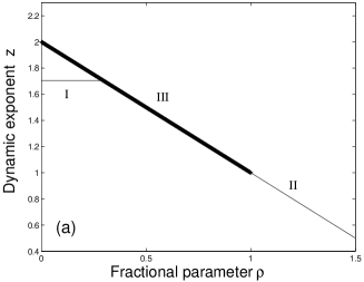
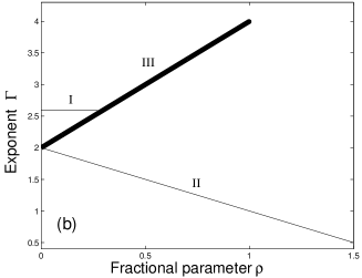
Figure 1: The values of the scaling exponents (a) $z$ and (b) $\Gamma$ as a function of the fractional parameter $\rho$, for uncorrelated noise ($\sigma=0$) in two-dimensions.

The described two-dimensional (and white-noise) scenario is quite typical and appears in other dimensions as well - namely there are usually three possible phases that are possible for different values of $\sigma$ with possible phase transitions between them (as in the usual KPZ scenario - the phase transition is controlled by the strength of the dimensionless coupling constant). More precisely, this picture extends up to the upper critical dimension of the original KPZ problem ($d_{uc}^{KPZ}$) where the first phase (phase I in Fig. 1) disappears (see the discussion below).

At this point, the full picture of possible solutions might seem too complex, so I want to suggest the following simple interpretation for the behavior of the Fractal KPZ equation. If you remember, the starting point of this discussion was the introduction of the fractional Laplacian into the KPZ equation. This immediately implies that faster relaxations are now possible (faster in the sense that a smaller dynamical exponent is expected) when compared with the Edwards-Wilkinson equation. However, it is well known that already the KPZ nonlinearity introduces faster relaxations (at least for dimensions lower than the upper critical dimension). Therefore, in the FKPZ system, the dynamics is controlled by the fastest ”component”: if the dynamical exponent of the classical KPZ system is smaller than $2-\rho$ then it dominates, otherwise the new fractional dynamical exponent $z=2-\rho$ controls the dynamics. However, at this point the picture gets a little bit more complicated (just like in the classical KPZ case), namely there are several possible phases with this new fractional dynamical exponent $z=2-\rho$, and the transition between these phases is controlled by the strength of dimensionless coupling constant.

These conclusions have an important implication for the upper critical dimension of the FKPZ model (i.e. the dimension above which the dynamical exponent is the same as that of the linear theory). Namely, it is turns out that the FKPZ equation always has an upper critical dimension that is determined by the relation $\Gamma_{0}\left({d_{uc}^{FKPZ}}\right)=d_{uc}^{FKPZ}+2\rho$ (or alternatively, using the roughness exponent $\alpha$ - the upper critical dimension is the dimension where $\alpha_{KPZ}\left({d_{uc}^{FKPZ}}\right)=\rho$). Notice, that this result does not dependent on the ongoing debate over the existence of the upper critical dimension for the KPZ system (see UCD98 -Marinari2002 ). Actually, it merely requires that the roughness exponent of the classical KPZ system becomes arbitrarily small in higher dimensions - an assumption that is generally accepted (only Tu Tu94 had a different conjecture).

As one can see, the results obtained using the Self-Consistent Expansion (SCE) are quite general, and cover all possible values of the relevant parameters ($\rho$ and $\sigma$) as well as dimensions. It is also easily verified that these results recover the exact result obtained at the beginning of this paper for the case $\rho=2\sigma$. This situation, suggest that the SCE method is generally appropriate when dealing with non-linear continuum equations.

Acknowledgement: I would like to thank Moshe Schwartz for useful discussions.

References

- (1) M. Kardar, G. Parisi and Y.-C. Zhang, Phys. Rev. Lett. 56, 889 (1986).
- (2) A.-L. Barabasi and H. E. Stanley, Fractal Concepts in Surface Growth (Cambridge Univ. Press, Cambridge, 1995).
- (3) J.A. Mann Jr. and W.A. Woyczynski, Physica A 291, 159 (2001).
- (4) G.L. Kellog, Phys. Rev. Lett. 72, 1662 (1994).
- (5) F. Family and T. Vicsek, J. Phys. A 18, L75 (1985).
- (6) M. Schwartz and S.F. Edwards, Europhys. Lett. 20, 301 (1992).
- (7) M. Schwartz and S.F. Edwards, Phys. Rev. E 57, 5730 (1998).
- (8) E. Katzav and M. Schwartz, Phys. Rev. E 60, 5677 (1999).
- (9) E. Medina, T. Hwa, M. Kardar and Y.C. Zhang, Phys. Rev. A 39, 3053 (1989).
- (10) J.R. Herring, Phys. Fluids 8, 2219 (1965); 9, 2106 (1966).
-
(11)
T. Ala-Nissila,
Phys. Rev. Lett. 80, 887 (1998).
J. M. Kim, ibid. 80, 888 (1998).
M. Lassig and H. Kinzelbach, ibid. 80, 889 (1998). - (12) E. Perlsman and M. Schwartz, Physica A 234, 523 (1996).
-
(13)
C. Castellano, M. Marsili and L. Pietronero,
Phys. Rev. Lett. 80, 3527 (1998).
C. Castellano, A. Gabrielli, M. Marsili, M.A. Munoz and L. Pietronero, Phys. Rev. E 58, 5209 (1998). - (14) T. Halpin-Healy, Phys. Rev. A 42, 711 (1990).
- (15) T. Blum and A. J. McKane, Phys. Rev. E 52, 4741 (1995).
-
(16)
J-P. Bouchaud and M. E. Cates,
Phys. Rev. E 47, 1455 (1993).
erratum), Phys. Rev. E 48, 653 (1993). - (17) E. Katzav and M. Schwartz, Physica A 309, 69 (2002).
- (18) J. Cook and B. Derrida, J. Phys. A 23, 1523 (1990).
- (19) F. Colaiori and M. A. Moore, Phys. Rev. Lett. 86, 3946 (2001).
- (20) E. Marinari, A. Pagnani, G. Parisi and Z. Rácz, Phys. Rev. E 65, 26136 (2002).
- (21) Y. Tu, Phys. Rev. Lett. 73, 3109 (1994).
- (22) R. Metzler, E.Barkai and J. Klafter, Phys. Rev. Lett. 82, 3563 (1999).
- (23) R. Metzler and J. Klafter, Chem. Phys. Lett. 321, 238 (2000).
- (24) R. Granek and J. Klafter, Europhys. Lett. 56, 15 (2001).
- (25) M. Sokolov, J. Klafter and A. Blumen, Phys. Rev. E 64, 21107 (2001).
- (26) H. Scher and E. Montroll, Phys. Rev. B 12, 2455 (1975).
- (27) Q. Gu, E. A. Schiff, S. Grebner and R. Schwartz, Phys. Rev. Lett. 76, 3196 (1996).
- (28) A. Klemm, H.-P. Müller and R. Kimmich, Phys. Rev. E 55, 4413 (1997).
- (29) F. Amblard, A. C. Maggs, B. Yurke, A. N. Pargellis and S. Leibler, Phys. Rev. Lett. 77, 4470 (1996).
- (30) M. Lässig, Nucl. Phys. B 448, 559 (1995).
- (31) K.J. Wiese, J. Stat. Phys. 93, 143 (1998).
- (32) E. Frey, U.C. Täuber and H.K. Janssen, Europhys. Lett. 47, 14 (1999).
- (33) H.K. Janssen, U.C. Täuber and E. Frey, Europhys. J. B 9, 491 (1999).
- (34) A. Kr. Chattapohadhyay and J. K. Bhattacharjee, Europhys. Lett. 42, 119 (1998).
- (35) E. Frey and U.C. Täuber, Phys. Rev. E 50, 1024 (1994).