Exactly solvable model of reactions on a random catalytic chain.

G.Oshanin¹, O.Bénichou² and A.Blumen³

¹ Laboratoire de Physique Théorique des Liquides,
Université Paris 6, 4 Place Jussieu, 75252 Paris, France

² Laboratoire de Physique de la Matière Condensée,
Collège de France, 11 Place M.Berthelot, 75252 Paris Cedex 05, France

³ Theoretische Polymerphysik,
Universität Freiburg, Hermann-Herder-Str. 3,
D-79104 Freiburg, Germany

In this paper we study a catalytically-activated $A+A\to 0$ reaction taking place on a one-dimensional regular lattice which is brought in contact with a reservoir of $A$ particles. The $A$ particles have a hard-core and undergo continuous exchanges with the reservoir, adsorbing onto the lattice or desorbing back to the reservoir. Some lattice sites possess special, catalytic properties, which induce an immediate reaction between two neighboring $A$ particles as soon as at least one of them lands onto a catalytic site. We consider three situations for the spatial placement of the catalytic sites: regular, $annealed$ random and $quenched$ random. For all these cases we derive $exact$ results for the partition function, and the disorder-averaged pressure per lattice site. We also present exact asymptotic results for the particles’ mean density and the system’s compressibility. The model studied here furnishes another example of a 1D Ising-type system with random multisite interactions which admits an exact solution.

Key Words: Random reaction/adsorption model, quenched and annealed disorder

1 Introduction.

Reactions involving particles which may recombine only when some third substance - the catalytic substrate - is present [1, 2], but otherwise remain chemically inactive, are ubiquitous in nature and also widely used in a variety of technological and industrial processes. Within the past two decades much effort has been put in understanding the peculiarities of such catalytically-activated reactions (CARs). In particular, considerable theoretical knowledge was gained from an extensive study of a particular reaction scheme - the CO-oxidation in the presence of metal surfaces with catalytic properties [3] (see also Ref.[4] for a recent review). Remarkably, Refs.[3] have substantiated the emergence of an essentially different behavior as compared to the predictions of the classical, formal-kinetics scheme and have shown that under certain conditions such collective phenomena as phase transitions or the formation of bifurcation patterns may take place [3]. Prior to these works on catalytic systems, anomalous behavior was amply demonstrated in other schemes [5, 6, 7], involving reactions on contact between two particles at any point of the reaction volume (i.e., ”completely” catalytic sysems). It was realized [5, 6, 7] that the departure from the text-book, formal-kinetic predictions is due to many-particle effects, associated with fluctuations in the spatial distribution of the reacting species. This suggests that, similar to such ”completely” catalytic reaction schemes, the behavior of the CARs may be influenced by many-particle effects.

Apart from many-particle effects, the behavior of the CARs might be affected by the very structure of the catalytic substrate, which often cannot be considered as being a well-defined geometrical object, but represents rather an assembly of mobile or localized catalytic sites or islands, whose spatial distribution is complex [1]. Metallic catalysts, for instance, are often disordered compact aggregates, the building blocks of which are imperfect crystallites with broken faces, kinks and steps. Usually only the steps are active in promoting the reaction. In porous materials with convoluted surfaces, such as, e.g., silica, alumina or carbons, the effective catalytic substrate is also only a portion of the total surface area because of the selective participation of different sites in reaction. Finally, for liquid-phase CARs the catalyst can consist of active groups attached to polymer chains in solution.

Such complex morphologies render the theoretical analysis difficult. There are only a few available studies which concern disordered substrates such as found in the CO-oxidation scheme; here the disorder is believed to affect mainly the particles’ adsorption and desorption [8, 9, 10, 11, 12, 13, 14, 15, 16]. On the other hand, for the situations in which the spatial distribution of the catalyst is random, only empirical approaches have been used, based mostly on heuristic concepts of effective reaction order or on phenomenological generalizations of the formal-kinetic ”law of mass action” (see, e.g., Refs.[1] and [2] for more details). The important outcome of such descriptions is that they provide an evidence of the existing correlations between the morphology of the chemically reactive environment and reaction kinetic and steady-state properties. On the other hand, their shortcoming is that they do not explain the mechanisms underlying the anomalous kinetic and stationary behavior. In this regard, exact analytical solutions of even somewhat idealized or simplified models, are already highly desirable since such studies may provide an understanding of the effects of different factors on the properties of the CARs.

In this paper we study the catalytically-activated annihilation $A+A\to 0$ reaction in a simple, one-dimensional model with different (regular or random) distributions of the catalysts, appropriate to the just mentioned situations with the catalytically-activated reactions assisted by the active groups attached to polymer chains. More specifically, we consider here the $A+A\to 0$ reaction on a one-dimensional regular lattice which is brought in contact with a reservoir of $A$ partilces. Some portion of the lattice sites (marked by crosses in Fig.1) possesses special ”catalytic” properties such that they induce an immediate reaction $A+A\to 0$, when at least one of two neighboring adsorbed $A$ particles sits on a catalytic site. In this case these two particles react and instantaneously leave the chain.

In regard to the distribution of the catalytic sites, we focus here on three different situations. First, we consider the case when the catalytic sites are placed periodically, forming a regular sublattice. Next, we turn to the disordered case. We analyse first the case of annealed disorder and furnish an exact solution. Lastly, we analyse the behavior in the most complex case of quenched disorder, for which situation an exact solution is also derived.

We note finally that the kinetics of $A+A\to 0$ reactions involving $\it diffusive$ $A$ particles which react upon encounters on randomly placed catalytic sites has been discussed already in Refs.[20, 21] and [22], and a rather surprising behavior has been found, especially in low-dimensional systems. A much simplier equilibrium model of an $A+A\to 0$ reaction on a 1D chain with randomly placed catalytic segments has been solved in Refs.[17] and [18], by noticing that here the average pressure per lattice site coincides exactly with the Lyapunov exponent of a product of random two-by-two matrices, obtained in Ref.[19]. Additionally, the steady-state properties of contact $A+A\to 0$ reactions between diffusive $A$ particles, or $A+A\to 0$ reactions between immobile $A$ particles reacting via long-range reaction probabilities in systems with external particles input have been presented in Refs.[23] and [24, 25], respectively, which analysis has revealed non-trivial ordering phenomena with anomalous input intensity dependence of the mean particle density. This anomalous behavior agrees with earlier experimental observations [26]. For completely catalytic 1D systems, the kinetics of $A+A\to 0$ reactions with immobile $A$ particles undergoing cooperative desorption has been discussed in Refs.[27, 28] and [29]. Exact solutions for $A+A\to 0$ reactions in 1D completely catalytic systems in which $A$ particles perform conventional diffusive or subdiffusive motion have been presented in Refs.[30] and [31], respectively.

The paper is structured as follows: In section 2 we formulate our model and introduce the basic notations. Next, in section 3 we focus on situations with regular placements of catalytic sites. We calculate exactly the partition function of the model, the pressure per site, and present as well explicit results for the particles’ mean density in the thermodynamic limit from which we determine the compressibility of the system. In section 4 we study the behavior of the system in the case of random $annealed$ distributions of the catalytic sites. We show that in this case the model reduces to a one-dimensional lattice gas with an effective three-particle repulsive interaction. We develop a combinatorial formulation of the model which allows us to obtain an exact solution. We present thus an exact expression for the disorder-averaged pressure, as well as exact asymptotic expansions for the mean particle density and the compressibility. In section 5 we turn to the very complex situation where the random distribution of catalytic sites is $quenched$. For this case, averaging the logarithm of the partition function over the states of the quenched random variables describing the catalytic properties of lattice sites, we find that the problem reduces in finite lattices with a fixed number of catalytic sites to an exact enumeration of all possible interconnected clusters. The weights of such clusters are calculated exactly in terms of a certain combinatorial procedure, and we find eventually an exact expression for the disorder-averaged pressure in the quenched disorder case. Additionally, we evaluate exact asymptotic expansions for the mean-particle density and the compressibility. We show that the behavior of these properties differs substantially, depending on whether the disorder is annealed or quenched. In particular, in systems with annealed disorder the mean particle density tends to unity when the chemical potential $\mu\to\infty$ for any $p<1$, where $p$ is the mean density of catalytic sites. On the other hand, mean particle density in the quenched disorder case tends to a finite value $(1-p+p^{2})/(1+p^{2})<1$ as $\mu\to\infty$. As well, in the $annealed$ disorder case the compressibility appears to be a non-monotonic function of $p$ for any $\mu$, while in the quenched disorder case the compressibility shows a non-monotonic behavior as a function of $p$ only for $\mu\leq\mu_{crit}=\beta^{-1}\ln(2)$, where $\beta^{-1}$ is the temperature. Lastly, in section 6 we conclude with a summary of results. Details of intermediate calculations are summarized in the appendices A,B and C.

2 The model

Consider a one-dimensional, regular lattice containing $N$ adsorption sites (Fig.1), which is brought in contact with a reservoir of identical, non-interacting, hard-core $A$ particles - a vapor phase, maintained at a constant chemical potential $\mu$. The $A$ particles from the vapor phase can adsorb onto vacant adsorption sites and desorb back to the reservoir. The occupation of the ”i”-th adsorption site is described by the Boolean variable $n_{i}$, such that

$$n_{i}=\left\{\begin{array}[]{ll}1,\mbox{ if the "i"-th site is occupied,}\\ 0,\mbox{ otherwise.}\end{array}\right.$$

For computational convenience, we also add two special, boundary sites $i=0$ and $i=N+1$, and stipulate that these sites are always unoccupied, $n_{0}=n_{N+1}=0$.

Figure 1: One-dimensional lattice of $N$ adsorption sites in contact with a vapor phase. The filled circles denote $A$ particles with hard-cores. The crosses denote the adsorption sites with catalytic properties. (a) denotes a ”forbidden” particle configuration. The sites $i=0$ and $i=N+1$ are always unoccupied and non-catalytic, i.e. $n_{0}=n_{N+1}=0$ and $\zeta_{0}=\zeta_{N+1}=0$.

Suppose next that some of the adsorption sites possess ”catalytic” properties (crosses in Fig.1) in the sense that they induce an immediate reaction $A+A\to 0$ between neighboring $A$ particles; that is, if at least one of two neighboring adsorbed $A$ particles sits on a catalytic site, these two particles react and instantaneously leave the chain (desorb back to the reservoir). To specify the catalytic sites, we introduce the quenched variable $\zeta_{i}$, so that

$$\zeta_{i}=\left\{\begin{array}[]{ll}1,\mbox{if the "i"-th site is catalytic, $i=1,2,\ldots,N$, }\\ 0,\mbox{ otherwise.}\end{array}\right.$$

The sites at the extremities of the chain are supposed to be non-catalytic, i.e. $\zeta_{0}=0$ and $\zeta_{N+1}=0$. As for the segment $[1,N]$, we will consider several possible ways of spatial placement of catalytic sites, namely, regular and random.

For a given distribution of catalytic sites, the partition function $Z_{N}(\zeta)$ of the system under study can be written as follows:

$$Z_{N}(\zeta)=\lim_{\lambda\to\infty}\sum_{\{n_{i}\}}\exp\Big{(}\beta\mu\sum_{i=1}^{N}n_{i}-\lambda\sum_{i=1}^{N}\zeta_{i}\;n_{i}\;(n_{i-1}+n_{i+1})\Big{)},$$ (1)

where the summation extends over all possible configurations $\{n_{i}\}$, $\mu$ is the chemical potential which accounts for the reservoir pressure and for the particles’ preference for adsorption. The parameter $\lambda$ stands for the catalytic activity, which is here taken to be infinitely large. Such a choice implies that the reaction between two neighboring $A$s, in which pair at least one of $A$s sits on a catalytic site, takes place instantaneously. Note that here $Z_{N}(\zeta)$ is a functional of the configuration $\zeta=\{\zeta_{i}\}$.

We stop to note that an analysis of general reaction and diffusion problems was previously done using effective Hamiltonians of spin systems. Examples are, e.g., the works by Doi [32], Zeldovitch and Ovchinnikov [33], Alcaraz et al [34] and Simon [35]. Our procedure here is different in that we consider equilibrium systems and take the limit $\lambda\to\infty$, which allows us to present the basic results in closed form.

Now, taking into account that

$$\lim_{\lambda\to\infty}\exp\Big{(}-\lambda\zeta_{i}n_{i}(n_{i-1}+n_{i+1})\Big{)}\equiv\Big{(}1-\zeta_{i}n_{i}n_{i-1}\Big{)}\Big{(}1-\zeta_{i}n_{i}n_{i+1}\Big{)},$$ (2)

and setting

$$z=\exp\Big{(}\beta\mu\Big{)},$$ (3)

we can rewrite eq.(1) as:

$$Z_{N}(\zeta)=\sum_{\{n_{i}\}}\prod_{i=1}^{N}z^{n_{i}}\Big{(}1-\zeta_{i}n_{i}n_{i-1}\Big{)}\Big{(}1-\zeta_{i}n_{i}n_{i+1}\Big{)}$$ (4)

Hence, any two neighboring sites $i$ and $i-1$ appear to be coupled by a factor $(1-n_{i}n_{i-1})$ when at least one of these sites is catalytic. These coupling factors are depicted in Fig.1 as arcs connecting neighboring sites and signify that configurations $\{n_{i}\}$ in which the occupation variables $n_{i}$ and $n_{i-1}$ assume simultaneously the value $1$ are excluded. We introduce now the notion of ”cluster”, as being a set of sites, all connected to each other consecutively by arcs. Thus, a $K$-cluster contains $K$ sites. Note that the boundary between adjacent clusters is given by a pair of two neighboring non-catalytic sites, i.e. by two consecutive variables $\zeta_{i}$ and $\zeta_{i+1}$ which are both equal to zero (see Fig.1). Now, the chain decomposes into disjunct clusters, and consequently, the partition function $Z_{N}(\zeta)$ factorizes into independent terms, such that each one depicts its corresponding cluster.

It may be also instructive to rewrite eq.(1) in terms of the Ising-type spin variables $\sigma_{i}=(2n_{i}-1)$, such that $\sigma_{i}=\pm 1$. In terms of these variables, $Z_{N}(\zeta)$ of eq.(1) reads:

$$Z_{N}(\zeta)=\lim_{\lambda\to\infty}\exp\Big{(}(\beta\mu-\lambda p)\frac{N}{2}\Big{)}\sum_{\{\sigma_{i}\}}\exp\Big{(}\sum_{i=1}^{N}\mu_{i}\sigma_{i}+\sum_{i=1}^{N}J_{i}\sigma_{i}\sigma_{i+1}\Big{)}$$ (5)

where $p$ denotes the mean density of catalytic sites, $p=N^{-1}\sum_{i}^{N}\zeta_{i}$, while

$$\mu_{i}=\frac{\beta\mu}{2}-\frac{\lambda}{4}(2\zeta_{i}+\zeta_{i-1}+\zeta_{i+1}),\;\;\;\text{and}\;\;\;J_{i}=-\frac{\lambda}{4}(\zeta_{i}+\zeta_{i+1}).$$ (6)

Consequently, the model under study can be also thought of as a version of a one-dimensional Ising-type model with site-dependent magnetic fields and site-dependent couplings (see, e.g., some seminal works [36, 37, 19], as well Refs.[38] and [39] for a recent review). Note, however, that in our case both the fields and the couplings are non-local, and that the local energy $\epsilon_{i}$, $\epsilon_{i}=-\mu_{i}\sigma_{i}-J_{i}\sigma_{i}\sigma_{i+1}$, can assume several different values, depending on the occupation variables of the neighboring sites and on their catalytic properties.

We close this section by mentioning the results of the conventional mean-field approach, which depicts the evolution of our system [1, 2]. Discarding correlations between the occupation of neighboring sites, i.e. setting $n_{i}=\overline{n}$ , one writes the following balance equation

$$\dot{\overline{n}}=-p{\cal K}\overline{n}^{2}+g_{ads}\left(1-\overline{n}\right)-g_{des}\overline{n},$$ (7)

where the overdot denotes the time derivative, ${\cal K}$ stands for the elementary reaction constant, $p$ is the mean density of catalytic sites (introduced to account for the reduction in the reaction rate due to the partial chain coverage by catalytic sites), while the second and the third terms on the rhs of eq.(7) correspond to the usual Langmuir adsorption/desorption events; here $g_{ads}$ and $g_{des}$ are the adsorption and desorption rates, respectively, $g_{ads}/g_{des}=z$.

Equation (7) has the following equilibrium solution

$$\overline{n}=\frac{\left(g_{ads}+g_{des}\right)}{2p{\cal K}}\left\{\sqrt{\frac{4p{\cal K}g_{ads}}{\left(g_{ads}+g_{des}\right)^{2}}+1}-1\right\}.$$ (8)

In the limit ${\cal K}\to\infty$, (which is the limit of interest in the present paper), and with $p$ and $g_{ads}$ kept finite one finds that $\overline{n}\to 0$; from eq.(8) $\overline{n}$ vanishes as $\overline{n}\sim\sqrt{g_{ads}/p{\cal K}}$. In the following we proceed to show that the actual behavior of the mean density of the $A$ particles turns out to be very different from eq.(8); this is due to the emerging correlations between the $A$ particles. Note also that in the limit ${\cal K}\equiv 0$ (suppressed reaction), one recovers from eq.(8) the classic Langmuir result $\overline{n}=z/(1+z)$ [1, 2].

3 Regular placement of catalytic sites.

To fix the ideas, consider first a situation in which the catalytic sites are placed periodically, with period $L$, so that $\zeta_{i}$ obeys:

$$\zeta_{i}=\delta(i,nL+1),\;\;\;\text{with}\;\;\;n=0,1,\ldots,\Big{[}\frac{N-1}{L}\Big{]},$$ (9)

where $[x]$ denotes the integer part of the number $x$, and $\delta(k,m)$ is the Kroneker-delta symbol,

$$\delta(k,m)=\frac{1}{2\pi i}\oint_{{\cal C}}\frac{\mathrm{d}\tau}{\tau^{1+k-m}}=\left\{\begin{array}[]{ll}1,\mbox{if $k=m$,}\\ 0,\mbox{ otherwise,}\end{array}\right.$$

where ${\cal C}$ stands for any closed contour which encircles the origin counterclockwise while $(k,m)\in\mathbb{Z}^{2}$.

Figure 2: Periodic placement of the catalytic sites with the period $L=4$. (a) denotes a forbidden particle configuration.

We have now to distinguish between two situations: namely, when $L\geq 3$ and when $L=1$ or $L=2$. In the former case, evidently, the factors $(1-\zeta_{i}n_{i}n_{i\pm 1})$ in eq.(4) are non-overlapping (see Fig.2); then the partition function decomposes into elementary three-clusters centered around each catalytic site and (possibly) into uncoupled, ”free” sites, i.e. sites unaffected by any of the factors $(1-\zeta_{i}n_{i}n_{i\pm 1})$. On the other hand, in the cases $L=1$ and $L=2$ we deal with totally interconnected clusters, spanning the entire chain, as one can deduce from Fig.3. In fact, the role of $L=1$ and $L=2$ is, chemically speaking, identical.

Figure 3: Periodic placement of the catalytic sites with the period $L=2$. In this case all sites are coupled by factors $(1-n_{i}n_{i-1})$ and hence the occupation variables of any two neighboring sites can not assume the value $1$ simultaneously; (a) denotes such ”forbidden” particle configurations.

3.1 Periodic case with $L\geq 3$.

In the case $L\geq 3$ the partition function in eq.(4) decomposes into the product

$$Z_{N}(\zeta)=Z_{N}^{(reg)}(L)=Z_{3}^{{\cal N}_{3}}\;Z_{2}^{{\cal N}_{2}}\;Z_{1}^{{\cal N}_{1}},$$ (10)

where the superscript ”(reg)” signifies that we deal with the regular case, and where $Z_{K}$, $K=1$, $K=2$ and $K=3$, are the partition functions of one-, two- and three-clusters, while ${\cal N}_{K}$, $K=1,2,3$, stands for the numbers of such clusters in the $N$-chain, respectively. Now:

$${\cal N}_{3}=\Big{[}\frac{N-1}{L}\Big{]}-\delta\Big{(}\frac{N-1}{L},\Big{[}\frac{N-1}{L}\Big{]}\Big{)};\;\;\;{\cal N}_{2}=1+\delta\Big{(}\frac{N-1}{L},\Big{[}\frac{N-1}{L}\Big{]}\Big{)},$$ (11)

and

$${\cal N}_{1}=N-2+\delta\Big{(}\frac{N-1}{L},\Big{[}\frac{N-1}{L}\Big{]}\Big{)}-3\Big{[}\frac{N-1}{L}\Big{]},$$ (12)

where we have used the evident ”conservation” law

$$3{\cal N}_{3}+2{\cal N}_{2}+{\cal N}_{1}=N.$$ (13)

Note, however, that the number of the two-clusters is not extensive, i.e., it does not grow with $N$: Such clusters can be present only on the boundaries, i.e., ${\cal N}_{2}=2$ when $(N-1)/L$ is an integer and ${\cal N}_{2}=1$ otherwise. Moreover,

$$Z_{1}=\sum_{\{n_{1}=0,1\}}z^{n_{1}}=(1+z);\;\;\;Z_{2}=\sum_{\{n_{1},n_{2}=0,1\}}z^{n_{1}+n_{2}}(1-n_{1}n_{2})=(1+2z),$$ (14)

and

$$Z_{3}=\sum_{\{n_{1},n_{2},n_{3}=0,1\}}z^{n_{1}+n_{2}+n_{3}}(1-n_{1}n_{2})(1-n_{2}n_{3})=(1+3z+z^{2}).$$ (15)

Consequently, in the case of a regular, periodic placement of catalytic sites with period $L$, $L\geq 3$, we can calculate the pressure $P^{(reg)}(L)$ per site from the relation:

$$\beta P^{(reg)}(L)=\lim_{N\to\infty}\frac{\ln Z_{N}^{(reg)}(L)}{N},$$ (16)

which yields:

$$\beta P^{(reg)}(L) = \lim_{N\to\infty}\Big{(}\frac{{\cal N}_{3}}{N}\ln Z_{3}-\frac{{\cal N}_{2}}{N}\ln Z_{2}-\frac{{\cal N}_{1}}{N}\ln Z_{1}\Big{)}=$$ (17)

$$= p\;\ln(1+3z+z^{2})+(1-3p)\;\ln(1+z),$$

where $p=1/L$ is the density of catalytic sites.

The averaged density of adsorbed particles obeys

$$n^{(reg)}(L)=\frac{1}{N}\overline{\sum_{i=1}^{N}n_{i}}=\frac{z}{N}\frac{d}{dz}\ln Z_{N}^{(reg)}(L),$$ (18)

and hence, in the limit $N\to\infty$ it follows that

$$n^{(reg)}(L)=(1-3p)\frac{z}{1+z}+p\frac{3z+2z^{2}}{1+3z+z^{2}}.$$ (19)

We stop to note that in the limit $p=0$ (i.e. that of a completely non-catalytic chain) eq.(19) reduces to the standard Langmuir result. On the other hand, when $p=1/3$ the number of free-sites in the periodic chain vanishes and the Langmuir contribution gets equal to zero; in this case the chain is composed totally of three-clusters. In this case, for very large $z$ the occupation of lattice sites by adsorbed molecules equals $2/3$, as it should.

Finally, we have that the compressibility $k_{T}$, defined as

$$\beta^{-1}k_{T}=\frac{1}{n^{2}}\frac{\partial n}{\partial\mu}=\frac{z}{n^{2}}\frac{\partial n}{\partial z}$$ (20)

obeys

$$\beta^{-1}k_{T}^{(reg)}(L)=\frac{1+6z+11z^{2}+6z^{3}+z^{4}-pz(8+8z+19z^{2})}{z(1+3z+z^{2}-4pz-pz^{2})^{2}}.$$ (21)

For $p=0$ the last equation reduces to the standard Langmuir result, $k_{T}^{(lan)}=\beta/z$.

3.2 Periodic cases with $L=1$ or $L=2$.

We note first that since $(1-n_{i}n_{i+1})^{2}=(1-n_{i}n_{i+1})$, we evidently have that

$$Z_{N}\equiv Z_{N}^{(reg)}(L=1)=Z_{N}^{(reg)}(L=2)=\left.\sum_{\{n_{i}\},i=1,\ldots,N}z^{\sum_{i=1}^{N}n_{i}}\prod_{i=1}^{N}\Big{(}1-n_{i}n_{i+1}\Big{)}\right|_{n_{N+1}=0}.$$ (22)

We hence conclude that the $L=1$ and the $L=2$ periodic systems are chemically equivalent.

Now, we focus on the derivation of the form of $Z_{N}$ according to eq.(22). To do this, we proceed as follows: performing first the averaging over the states of the variable $n_{N}$, we have that $Z_{N}$ can be written as

$$Z_{N}=Z_{N-1}+z\sum_{\{n_{i}\},i=1,\ldots,N-1}z^{\sum_{i=1}^{N-1}n_{i}}\prod_{i=1}^{N-2}\Big{(}1-n_{i}n_{i+1}\Big{)}\Big{(}1-n_{N-1}\Big{)},$$ (23)

where $Z_{N-1}$ obeys

$$Z_{N-1}=\left.\sum_{\{n_{i}\},i=1,\ldots,N-1}z^{\sum_{i=1}^{N-1}n_{i}}\prod_{i=1}^{N-1}\Big{(}1-n_{i}n_{i+1}\Big{)}\right|_{n_{N}=0},$$ (24)

and is hence the partition function of a chain consisting of $N-1$ sites. We notice next that the second term on the rhs of eq.(23) vanishes when $n_{N-1}=1$; thus it can be written as

$$\sum_{\{n_{i}\},i=1,\ldots,N-1}z^{\sum_{i=1}^{N-1}n_{i}}\prod_{i=1}^{N-2}\Big{(}1-n_{i}n_{i+1}\Big{)}\Big{(}1-n_{N-1}\Big{)}=$$ (25)

$$= \left.\sum_{\{n_{i}\},i=1,\ldots,N-2}z^{\sum_{i=1}^{N-2}n_{i}}\prod_{i=1}^{N-2}\Big{(}1-n_{i}n_{i+1}\Big{)}\right|_{n_{N-1}=0},$$

where the expression on the right-hand-side is, evidently, the partition function of a chain containing $N-2$ sites. Consequently, the partition function of an $N$-site chain obeys the following recursion:

$$Z_{N}=Z_{N-1}+zZ_{N-2}$$ (26)

whose first three terms are given by eqs.(14) and (15).

Next, to determine $Z_{N}$ explicitly for arbitrary $N$ we introduce the following generating function

$${\cal H}(\tau)=\sum_{N=1}^{\infty}Z_{N}\tau^{N}.$$ (27)

Then, multiplying both sides of eq.(26) by $\tau^{N-2}$ and performing the summation, we obtain the following explicit result for ${\cal H}(\tau)$:

$${\cal H}(\tau) = \Big{(}z\tau^{2}+(1+z)\tau\Big{)}\Big{(}1-\tau-z\tau^{2}\Big{)}^{-1}=$$ (28)

$$= \frac{\Big{(}z\tau^{2}+(1+z)\tau\Big{)}}{\sqrt{1+4z}}\Big{(}\frac{1}{\tau+\tau_{1}}+\frac{1}{\tau_{2}-\tau}\Big{)},$$

where $\tau_{1}$ and $\tau_{2}$ are given by

$$\tau_{1}=\frac{1}{2z}\Big{(}\sqrt{1+4z}+1\Big{)}$$ (29)

and

$$\tau_{2}=\frac{1}{2z}\Big{(}\sqrt{1+4z}-1\Big{)}.$$ (30)

Next, expanding the terms in the second line on the rhs of eq.(28) in a Taylor series in powers of $\tau$ and gathering terms entering with the same power, we find that $Z_{N}$ obeys

$$Z_{N}=\frac{1+2z+\sqrt{1+4z}}{2\sqrt{1+4z}\;\tau_{2}^{N}}\;{\cal L}_{N},$$ (31)

where

$${\cal L}_{N}=\Big{(}1-(-1)^{N}\frac{(1+2z-\sqrt{1+4z})}{(1+2z+\sqrt{1+4z})}\Big{(}\frac{\tau_{2}}{\tau_{1}}\Big{)}^{N}\Big{)}$$ (32)

We recall that the $Z_{N}$ are, of course, polynomial functions of the activity $z$; expanding the rhs of eq.(31) in powers of $z$, we get

$$Z_{N}=\sum_{l=0}^{[(N+1)/2]}{N-l+1\choose l}z^{l},$$ (33)

where ${N\choose l}$ denote the binomial coefficients,

$${N\choose l}=\left\{\begin{array}[]{ll}\displaystyle N!/l!(N-l)!,\mbox{for $N\geq l$,}\\ 0,\mbox{ otherwise.}\end{array}\right.$$

For large values of $z$, it might be more convenient to use another representation; subtracting in eq.(33) $z^{(N+1)/2}$ and summing up the remaining terms, we find that $Z_{N}$ are given by

$$Z_{N}=z^{(N+1)/2}F_{N+2}(1/\sqrt{z}),$$ (34)

where $F_{n}(x)$ are the Fibonacci polynomials [40], defined explicitly by

$$F_{n}(x)=\sum_{l=0}^{[(n-1)/2]}{n-l-1\choose l}x^{n-2l-1}.$$ (35)

Finally, noticing that for $z<\infty$ one has $(\tau_{2}/\tau_{1})<1$ and hence, that $(\tau_{2}/\tau_{1})^{N}$ vanishes exponentially with $N$ as $N\to\infty$, we find in the cases when $L=1$ and $L=2$ that the pressure per site obeys, using eq.(16):

$$\beta P^{(reg)}(L=1\,{\rm or}\,2)=\ln\Big{(}\frac{\sqrt{1+4z}+1}{2}\Big{)},$$ (36)

while the average density in an infinite chain is, using eq.(18):

$$n^{(reg)}(L=1\,{\rm or}\,2)=1-\frac{2z}{1+4z-\sqrt{1+4z}}.$$ (37)

In the limit $z=\infty$, the roots $\tau_{1}$ and $\tau_{2}$ are equal, $\tau_{1}=\tau_{2}$, this signals the emergence of long-range order. Actually, in this case $n^{(reg)}(L=1\,{\rm or}\,2)=1/2$ and the particles’ distribution on the lattice is periodic.

Finally, to close this section, we derive the compressibility of the particle phase. In the thermodynamic limit, for regular placement of the catalytic sites with the period $L=1$ or $L=2$ it obeys:

$$\beta^{-1}k_{T}^{(reg)}(L=1\,{\rm or}\,2)=\frac{2z}{\sqrt{1+4z}(1+2z-\sqrt{1+4z})}.$$ (38)

Note that contrary to the expression in eq.(21) which holds for $L\geq 3$, here $k_{T}^{(reg)}(L=1\,{\rm or}\,2)$ is a non-analytic function of the activity $z$ when $z\to\infty$.

4 Random placement of catalytic sites. Annealed disorder.

Consider next the situation with $\it annealed$ disorder, which is realized, for instance, when the catalytic property may move (diffuse) very quickly. In this case, the disorder-average pressure $P^{(ann)}(p)$ per site and the average density are given by, respectively,

$$P^{(ann)}(p)=\lim_{N\to\infty}\frac{\ln\left<Z_{N}(\zeta)\right>}{\beta N},$$ (39)

and

$$n^{(ann)}(p)=\frac{1}{N}\overline{\sum_{i=1}^{N}n_{i}}=\beta z\frac{d}{dz}P^{(ann)}(p),$$ (40)

where $Z_{N}(\zeta)$ is again the partition function of eq.(1).

We can now average directly the partition function in eq.(1) over the placement of the sites with catalytic property:

$$\left<Z_{N}(\zeta)\right> = \lim_{\lambda\to\infty}\sum_{\{n_{i}\}}\exp\Big{(}\beta\mu\sum_{i=1}^{N}n_{i}\Big{)}\left<\exp\Big{(}-\lambda\sum_{i=1}^{N}\zeta_{i}n_{i}(n_{i-1}+n_{i+1})\Big{)}\right>=$$ (41)

$$= \lim_{\lambda\to\infty}\sum_{\{n_{i}\}}\exp\Big{(}\beta\mu\sum_{i=1}^{N}n_{i}\Big{)}\prod_{i=1}^{N}\left<\exp\Big{(}-\lambda\zeta_{i}n_{i}(n_{i-1}+n_{i+1})\Big{)}\right>=$$

$$= \sum_{\{n_{i}\}}z^{\sum_{i=1}^{N}n_{i}}\lim_{\lambda\to\infty}\prod_{i=1}^{N}\Big{(}p\exp\Big{(}-\lambda n_{i}(n_{i-1}+n_{i+1})\Big{)}+1-p\Big{)}.$$

Noticing next that

$$\lim_{\lambda\to\infty}\Big{(}p\exp\Big{(}-\lambda n_{i}(n_{i-1}+n_{i+1})\Big{)}+1-p\Big{)}=\left\{\begin{array}[]{ll}1-p,\mbox{ if $n_{i}(n_{i-1}+n_{i+1})>0$,}\\ 1,\mbox{if $n_{i}(n_{i-1}+n_{i+1})=0$,}\end{array}\right.$$

and hence, that

$$\lim_{\lambda\to\infty}\Big{(}p\exp\Big{(}-\lambda n_{i}(n_{i-1}+n_{i+1})\Big{)}+1-p\Big{)}=(1-p)^{\displaystyle n_{i}(1-(1-n_{i-1})(1-n_{i+1}))},$$ (42)

we find that the averaged partition function in eq.(1) attains the form

$$\left<Z_{N}(\zeta)\right>=\sum_{\{n_{i}\}}z^{\sum_{i=1}^{N}n_{i}}(1-p)^{\sum_{i=1}^{N}\Psi_{i}},$$ (43)

where $\Psi_{i}$ is a Boolean variable:

$$\Psi_{i}=(n_{i}n_{i+1}+n_{i}n_{i-1}-n_{i-1}n_{i}n_{i+1})=\left\{\begin{array}[]{ll}1,\mbox{ if $n_{i}(n_{i-1}+n_{i+1})>0$,}\\ 0,\mbox{if $n_{i}(n_{i-1}+n_{i+1})=0$.}\end{array}\right.$$

Evidently, $\Psi_{i}$ is non-local and depends on the environment of the ”i”-th site. As a matter of fact, the local energy $\epsilon_{i}$ at the ”i”-th site, $\epsilon_{i}=-\beta\mu n_{i}-\ln(1-p)(n_{i}n_{i+1}+n_{i}n_{i-1}-n_{i-1}n_{i}n_{i+1})$, assumes $8$ different values depending on $n_{i-1}$, $n_{i}$ and $n_{i+1}$. Before we proceed further, it might be also instructive to rewrite eq.(43) in terms of the spin variables $\sigma_{i}$. Then eq.(43) takes the form

$$\left<Z_{N}(\zeta)\right> = \exp\Big{(}(\beta\mu+\frac{3}{4}\ln(1-p))\frac{N}{2}\Big{)}\sum_{\{\sigma_{i}\}}\exp\Big{(}\beta\mu^{\prime}\sum_{i=1}^{N}\sigma_{i}+J_{1}\sum_{i=1}^{N}\sigma_{i}\sigma_{i+1}-$$ (44)

$$- J_{2}\sum_{i=1}^{N}\sigma_{i-1}\sigma_{i+1}-J_{3}\sum_{i=1}^{N}\sigma_{i-1}\sigma_{i}\sigma_{i+1}\Big{)},$$

where

$$\mu^{\prime}=\mu+\frac{5}{8\beta}\ln(1-p);\;\;\;J_{1}=\frac{\ln(1-p)}{4}<0;\;\;\;\text{and}\;\;\;J_{2}=J_{3}=\frac{\ln(1-p)}{8}<0.$$ (45)

As one may notice, the expression in eq.(44) represents a combination of two well-known Ising-type models: namely, the first three terms in the exponent define the antiferromagnetic ANNNI (axial next-nearest neighbor Ising) chain [41]. In our case, the competition ratio $k=J_{2}/J_{1}$ equals $k=1/2$, which is, in fact, a non-trivial special point (the so-called multiphase point [42]) of the ANNNI model. On the other hand, the fourth term in the exponent corresponds to the three-spin interaction model [43]. Both models have been extensively studied within the last two decades in various contexts [42, 43] and show interesting equilibrium and dynamic properties, see e.g., Refs.[44, 45]. We are, however, unaware of an exact solution of the one-dimensional combined model of eq.(44). Below we will furnish such an exact solution using a combinatorial approach.

Note now that $\Psi_{i}$ always equals zero for unoccupied sites, $(n_{i}=0)$, but attains the value $\Psi_{i}=1$ only for occupied sites, $(n_{i}=1)$, which have at least one (or two) occupied neighboring sites (see Fig.4).

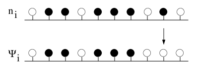
Figure 4: Values of the variable $\Psi_{i}$ corresponding to a given configuration $\{n_{i}\}$.

Otherwise, for isolated occupied sites (elementary sequences with $(n_{i-1}=0,n_{i}=1,n_{i+1}=0)$) the variable $\Psi_{i}$ equals $0$. Consequently, for any given realization $\{n_{i}\}$, one has that

$$\sum_{i=1}^{N}\Psi_{i}={\cal N}_{+}[\{n_{i}\}]-{\cal N}_{is}[\{n_{i}\}],$$ (46)

where ${\cal N}_{+}[\{n_{i}\}]$ is the number of lattice sites on which (in a given realization $\{n_{i}\}$) the occupation variable $n_{i}$ assumes the value $1$, while ${\cal N}_{is}[\{n_{i}\}]$ is the realization-dependent number of isolated occupied sites (elementary cells of the form $(0,1,0)$). Hence, the partition function in eq.(43) can be rewritten as

$$\left<Z_{N}(\zeta)\right>=\sum_{\{n_{i}\}}\Big{(}z(1-p)\Big{)}^{{\cal N}_{+}[\{n_{i}\}]}(1-p)^{-{\cal N}_{is}[\{n_{i}\}]}$$ (47)

Next, ordering the entire set of $2^{N}$ different realizations $\{n_{i}\}$ with respect to the total number of adsorbed particles which they contain, i.e. ${\cal N}_{+}[\{n_{i}\}]$, we can recast eq.(47) into the form:

$$\left<Z_{N}(\zeta)\right>=\sum_{{\it N}_{+}=0}^{N}\Big{(}z(1-p)\Big{)}^{{\it N}_{+}}\;\sum_{m=0}^{N-{\it N}_{+}+1}(1-p)^{-m}M_{m}({\it N}_{+}|N),$$ (48)

where $M_{m}({\it N}_{+}|N)$ stands for the number of realizations $\{n_{i}\}$ that have a fixed ${\it N}_{+}$ and contain $\it exactly$ $m$ elementary cells $(0,1,0)$.

4.1 Calculation of $M_{m}({\it N}_{+}|N)$.

To evaluate $M_{m}({\it N}_{+}|N)$ we now proceed as follows. Let us consider a given realization $\{n_{i}\}$ with ${\it N}_{+}$ filled (and ${\it N}_{-}=N-{\it N}_{+}$ vacant) sites and specify the lattice positions of the vacant sites by introducing a set of intervals $\{{\it l}_{j}\}$, $j=1,\ldots,{\it N}_{-}+1$, such that the interval ${\it l}_{1}$ connects a boundary site $i=0$ with the first vacant site, the interval ${\it l}_{2}$ connects the first vacant site with the second one, and etc, while the last interval ${\it l}_{\it N_{-}{\rm+1}}$ connects the last vacant site with the boundary site $i=N+1$ (see Fig.5).

These intervals, which uniquely define the positions of the vacant sites in each given realization $\{n_{i}\}$, obey the ”conservation law”:

$${\it l}_{1}+{\it l}_{2}+{\it l}_{3}+\;\ldots\;+{\it l}_{\it N_{-}{\rm+1}}=N+1$$ (49)

Then, since each interval containing exactly two lattice units corresponds to an isolated occupied site, $M_{m}({\it N}_{+}|N)$ equals the number of different solutions of eq.(49), constrained by the condition that in each sequence $\{{\it l}_{i}\}$ obeying eq.(49) $m$ of the ${\it N}_{-}+1$ intervals are equal to $2$, while the rest can assume any value except $2$. Hence, $M_{m}({\it N}_{+}|N)$ can be represented as

$$M_{m}({\it N}_{+}|N)={{\it N}_{-}+1\choose m}\;{\it P}_{m}({\it N}_{+}|N).$$ (50)

Here the binomial coefficient accounts for all possible choices of $m$ intervals from the set of ${\it N}_{-}+1$ intervals, while ${\it P}_{m}({\it N}_{+}|N)$ stands for the number of different solutions of the equation

$${\it l}_{1}+{\it l}_{2}+{\it l}_{3}+\;\ldots\;+{\it l}_{{\it N}_{-}-m+1}=N-2m+1,$$ (51)

where each of intervals ${\it l}_{k}$, $k=1,2,\ldots,{\it N}_{-}-m+1$, can assume one of the values ${\it l}_{k}=1,3,4,5,\ldots$.

Figure 5: Definition of a given configuration $\{n_{i}\}$ in terms of the intervals $\{{\it l}_{i}\}$ connecting sequentially unoccupied lattice sites.

Making use of the integral representation of the lattice delta-function in eq.(3), we can write ${\it P}_{m}({\it N}_{+}|N)$ as

$${\it P}_{m}({\it N}_{+}|N)=\frac{1}{2\pi i}\oint_{{\cal C}}\frac{d\tau}{\tau}\;\tau^{-(N-2m+1)}\Big{\{}\hat{\sum_{{\it l}_{\rm 1}}}\;\ldots\;\hat{\sum_{{\it l}_{{\it N}_{-}-m+1}}}\tau^{\displaystyle\Big{(}{\it l}_{1}+{\it l}_{2}+{\it l}_{3}+\;\ldots\;+{\it l}_{{\it N}_{-}-m+1}\Big{)}}\Big{\}},$$ (52)

where the hat above the summation symbol signifies that summation runs over all possible values $l_{k}=1,3,\ldots,\infty$, excluding the value $l_{k}=2$. Performing the summation, we find

$${\it P}_{m}({\it N}_{+}|N)=\frac{1}{2\pi i}\oint_{{\cal C}}\;\frac{d\tau}{\tau}\;\tau^{\displaystyle\Big{(}{\it N}_{+}-m\Big{)}}\;S_{\tau}^{N-{\it N}_{+}+1-m},$$ (53)

where

$$S_{\tau}=\left(\Big{(}1-\tau\Big{)}^{-1}-\tau\right).$$ (54)

4.2 Explicit form of $\left<Z_{N}(\zeta)\right>$.

Substituting eqs.(53) and (50) into eq.(48), we find that the partition function obeys

$$\left<Z_{N}(\zeta)\right>=\frac{1}{2\pi i}\oint_{{\cal C}}\;\frac{d\tau}{\tau}\;S_{\tau}^{N+1}\;\sum_{{\it N}_{+}=0}^{N}\Big{(}\frac{z(1-p)}{\tau S_{\tau}}\Big{)}^{{\it N}_{+}}\;\sum_{m=0}^{{\it N}_{-}+1}{{\it N}_{-}+1\choose m}\;\Big{(}\frac{\tau}{(1-p)S_{\tau}}\Big{)}^{m},$$ (55)

which yields, upon summing over $m$ and ${\it N}_{+}$, the following result

$$\left<Z_{N}(\zeta)\right> = \frac{2(1-p)}{9(-Q)p}\Big{\{}-\frac{1-3\sqrt{-Q}\cos\Big{(}\displaystyle\frac{1}{3}\arccos\Big{(}R/\sqrt{-Q^{3}}\Big{)}\Big{)}}{\displaystyle 1+2\cos\Big{(}\frac{2}{3}\arccos\Big{(}R/\sqrt{-Q^{3}}\Big{)}\Big{)}}\Big{(}\displaystyle\frac{z(1-p)}{t_{1}}\Big{)}^{N+2}+$$ (56)

$$+ \frac{1+3\sqrt{-Q}\sin\Big{(}\displaystyle\frac{1}{3}\arcsin\Big{(}R/\sqrt{-Q^{3}}\Big{)}\Big{)}}{2\sin\Big{(}\displaystyle\frac{\pi}{6}+\frac{2}{3}\arccos\Big{(}R/\sqrt{-Q^{3}}\Big{)}\Big{)}-1}\Big{(}\displaystyle\frac{z(1-p)}{t_{2}}\Big{)}^{N+2}-$$

$$- \frac{\displaystyle 1+3\sqrt{-Q}\sin\Big{(}\displaystyle\frac{1}{3}\arcsin\Big{(}R/\sqrt{-Q^{3}}\Big{)}\Big{)}}{\displaystyle 1-2\sin\Big{(}\frac{\pi}{6}-\frac{2}{3}\arccos\Big{(}R/\sqrt{-Q^{3}}\Big{)}\Big{)}}\Big{(}\displaystyle\frac{z(1-p)}{t_{3}}\Big{)}^{N+2}\Big{\}},$$

where $R$ and $Q$ are auxiliary functions, which obey

$$Q=-\frac{1}{9}-\frac{(1-p)}{3p}(1+z(1-p))\leq 0,$$ (57)

and

$$R=\frac{1}{27}+\frac{1}{6}\Big{(}\frac{(1-p)}{p}(1+z(1-p))-\frac{3z(1-p)^{2}}{p}\Big{)}.$$ (58)

Equation (56) defines $\left<Z_{N}(\zeta)\right>$ for arbitrary values of $p$, $z$ and chain’s length $N$. The derivation of eq.(56) is presented in Appendix A.

4.3 The thermodynamic limit $N\to\infty$.

We turn next to the thermodynamic limit aiming to calculate the disorder-averaged pressure per site in the $annealed$ disorder case and the mean density of adsorbed particles. In the limit $N\to\infty$ only the smallest root in absolute value matters. To select the appropriate root, it suffices to plot the combination $(t_{i}-1/3)/2\sqrt{-Q}$, $i=1,2,3$, versus the variable $x=R/\sqrt{-Q^{3}}$, which is defined on the interval $[-1,1]$. This plot is presented in Fig.6 and shows that the smallest root is $t=t_{2}$.

Figure 6: Plot of $(t_{i}-1/3)/2\sqrt{-Q}$, $i=1,2,3$, versus the variable $X=R/\sqrt{-Q^{3}}$. The dotted line $(1)$ gives $(t_{1}-1/3)/2\sqrt{-Q}$, the solid line $(2)$ gives $(t_{2}-1/3)/2\sqrt{-Q}$, and the dashed line $(3)$ gives $(t_{3}-1/3)/2\sqrt{-Q}$, respectively.

Consequently, taking into account that

$$\frac{1+3\sqrt{-Q}\sin\Big{(}\displaystyle\frac{1}{3}\arcsin\Big{(}R/\sqrt{-Q^{3}}\Big{)}\Big{)}}{2\sin\Big{(}\displaystyle\frac{\pi}{6}+\frac{2}{3}\arccos\Big{(}R/\sqrt{-Q^{3}}\Big{)}\Big{)}-1}\geq 0,$$ (59)

is positive definite, we find from eq.(39) that the pressure per site is given by

$$\beta P^{(ann)}(p) = \ln\Big{(}\frac{z(1-p)}{t_{2}}\Big{)}=$$ (60)

$$= -\ln\left(\frac{\Big{(}1-6\sqrt{-Q}\sin\Big{(}\displaystyle\frac{1}{3}\arcsin\Big{(}R/\sqrt{-Q^{3}}\Big{)}\Big{)}\Big{)}}{3z(1-p)}\right),$$

which expression determines $P^{(ann)}(p)$ for arbitrary values of the parameters $p$ and $z$.

Consider now the form of $P^{(ann)}(p)$ in the limits $p\to 0$ and $p\sim 1$. In the limit of a vanishingly small concentration of catalytic sites, we have from eq.(60) that:

$$\beta P^{(ann)}(p)=\ln(1+z)-\frac{z^{2}(2+z)}{\beta(1+z)^{3}}p+{\mathcal{O}}\Big{(}p^{2}\Big{)}.$$ (61)

Note that the first term in the last equation is, as it should be, just the standard Langmuir adsorption isotherm.

In the case $p\sim 1$, we expand first $t_{2}/z(1-p)$ in powers of $(1-p)$. This yields,

$$\frac{t_{2}}{z(1-p)}=\frac{\sqrt{1+4z}-1}{2z}-\frac{(1+z)\sqrt{1+4z}-3z-1}{2z\sqrt{1+4z}}(1-p)^{2}+{\mathcal{O}}\Big{(}(1-p)^{3}\Big{)},$$ (62)

which expansion, as one can check by comparing the first and the second terms in eq.(62), makes sense only when $(1-p)\ll(4/z)^{1/4}$. As a matter of fact, $p=1$ has here a special role, as will be shown in the following. Then, we find that the pressure per site is

$$\beta P^{(ann)}(p)=\ln\Big{(}\frac{\sqrt{1+4z}+1}{2}\Big{)}+\frac{4z^{2}+5z-3z\sqrt{1+4z}+1-\sqrt{1+4z}}{(\sqrt{1+4z}-1)(1+4z)}(1-p)^{2}+{\mathcal{O}}\Big{(}(1-p)^{3}\Big{)}$$ (63)

Note now that the first term in eq.(63), which defines the disorder-averaged pressure per site in the limit $p=1$, coincides exactly with the result we obtained earlier in the case of a regular placement of catalytic sites with the period $L=1$ (or $L=2$), eq.(36). As a matter of fact, one could notice that the partition function in the annealed-disorder case, eq.(48), will coincide for $p=1$ with the partition function for the regular case, eqs.(31) and (32), by just analysing the behavior of the coefficients $M_{m}({\it N}_{+}|N)$, eqs.(50) and (53). To show this, we note first that from eqs.(50) and (53) one has that $M_{m}({\it N}_{+}|N)\equiv 0$ for $m>{\it N}_{+}$. This is, of course, quite evident, if we recall that $M_{m}({\it N}_{+}|N)$ stands for the number of realizations $\{n_{i}\}$ having a fixed number ${\it N}_{+}$ of adsorbed particles and a fixed number $m$ of elementary cells containing one adsorbed particle surrounded by two vacant sites: hence, the number of realizations $\{n_{i}\}$ in which $m$ exceeds ${\it N}_{+}$ equals zero. Further on, one notices that when $p=1$, in eq.(48) only the terms $M_{m={\it N}_{+}}({\it N}_{+}|N)$ with ${\it N}_{+}\leq{\it N}_{-}+1=N+1-{\it N}_{+}$ matter. Hence eq.(48) becomes

$$\left<Z_{N}(\zeta)\right>=\sum_{{\it N}_{+}=0}^{[(N+1)/2]}M_{{\it N}_{+}}({\it N}_{+}|N)\;z^{{\it N}_{+}},$$ (64)

where

$$M_{m={\it N}_{+}}({\it N}_{+}|N)=\frac{1}{2\pi i}{{\it N}_{-}+1\choose{\it N}_{+}}\oint_{{\cal C}}\frac{d\tau}{\tau}S_{\tau}^{{\it N}_{-}+1-{\it N}_{+}}=$$ (65)

$$= \frac{1}{2\pi i}{{\it N}_{-}+1-{\it N}_{+}\choose{\it N}_{+}}\oint_{{\cal C}}\frac{d\tau}{\tau}\Big{(}1+\sum_{k=2}^{\infty}\tau^{k}\Big{)}^{{\it N}_{-}+1-{\it N}_{+}}\equiv{{\it N}_{-}+1-{\it N}_{+}\choose{\it N}_{+}}$$

On comparing eqs.(64) and (65) with eq.(33), we have in the limit $p=1$ that the partition function, (and hence, the pressure per site), in the annealed disorder case coincides with the partition function of a chain on which the catalytic sites are placed regularly with period $L=1$.

Finally, differentiating eq.(60) with respect to the variable $z$ and making use of eq.(40), we find that in the annealed disorder case the average density of adsorbed particles obeys:

$$n^{(ann)}(p)=1+\frac{3z(1-p)^{2}}{1-6\sqrt{-Q}\sin\Big{(}\displaystyle\frac{1}{3}\arcsin\Big{(}R/\sqrt{-Q^{3}}\Big{)}\Big{)}}\times$$ (66)

$$\times \Big{[}A\sin\Big{(}\frac{1}{3}\arcsin\Big{(}R/\sqrt{-Q^{3}}\Big{)}\Big{)}+\frac{B}{\sqrt{1+R^{2}/Q^{3}}}\cos\Big{(}\frac{1}{3}\arcsin\Big{(}R/\sqrt{-Q^{3}}\Big{)}\Big{)}\Big{]},$$

where

$$A=\Big{(}p(3zp^{2}-2p(1+3z)+3(1+z))\Big{)}^{-1/2},$$ (67)

and

$$B=\frac{3}{2}\frac{(2zp^{2}+p(5-4z)+2z-7)}{\Big{(}3zp^{2}-2p(1+3z)+3(1+z)\Big{)}^{2}}.$$ (68)

Note that the result in eq.(66) differs from the mean-field prediction $\overline{n}\equiv 0$, which follows from eq.(8) for instantaneous reactions, ${\cal K}=\infty$.

In Fig.8 we present a plot of $n^{(ann)}(p)$ versus $p$ for different values of the activity $z$. In Fig.8 we also compare the behavior of $n^{(ann)}(p)$ with the behavior found in the case of quenched disorder (see the next section). In the limits $p\ll 1$ and $p\sim 1$, we find that $n^{(ann)}(p)$ follows, respectively,

$$n^{(ann)}(p)=\frac{z}{1+z}-\frac{(4+z)z^{2}}{(1+z)^{4}}p+{\mathcal{O}}\left(p^{2}\right),$$ (69)

and

$$n^{(ann)}(p)=1-\frac{2z}{1+4z-\sqrt{1+4z}}+\frac{2z^{2}}{(1+4z)^{3/2}}(1-p)^{2}+{\mathcal{O}}\left((1-p)^{3}\right).$$ (70)

Note that the first term in eq.(69) is, as it should be, just the Langmuir adsorbtion isotherm, while the first term in eq.(70) coincides with our earlier result for the average density of adsorbed particles on the periodic chain with $L=1$ or $L=2$, see eq.(37).

Lastly, we analyse the behavior of the compressibility $k_{T}^{(ann)}(p)$ for the annealed disorder situation:

$$\beta^{-1}k_{T}^{(ann)}(p)=\frac{z}{(n^{(ann)}(p))^{2}}\frac{\partial n^{(ann)}(p)}{\partial z}.$$ (71)

We find that $k_{T}^{(ann)}(p)$ shows the following asymptotical behavior: For $p\ll 1$ we have

$$\beta^{-1}k_{T}^{(ann)}(p)=\frac{1}{z}+\frac{z(7+z)}{(1+z)^{3}}p+{\cal O}\Big{(}p^{2}\Big{)},$$ (72)

while for $p\sim 1$ the compressibility obeys

$$\beta^{-1}k_{T}^{(ann)}(p)=\beta^{-1}k_{T}^{(reg)}(L=1\,{\rm or}\,2)+\frac{4z^{2}}{(1+4z)^{3/2}}(1-p)^{2}+{\cal O}\Big{(}(1-p)^{3}\Big{)}.$$ (73)

Here $k_{T}^{(reg)}(L=1\,{\rm or}\,2)$ is as previously defined, eq.(38), and represents the compressibility of a completely catalytic chain. Note that the result in eq.(73) signifies that in the annealed disorder case the compressibility is a non-monotonic function of the mean density $p$ of catalytic sites. This can be seen immediately if one notices that, first, for any fixed $z$, one has $k_{T}^{(reg)}(L=1\,{\rm or}\,2)\geq k_{T}^{(lan)}=\beta/z$, (or in other words, that for any fixed $z$ the compressibility of a non-catalytic (Langmuir) system is always smaller than the compressibility of a completely catalytic system) and second, that $k_{T}^{(ann)}(p)$ approaches $k_{T}^{(reg)}(L=1\,{\rm or}\,2)$ from above, since the function $4z^{2}/(1+4z)^{3/2}$ is always positive.

We close this section with some comments concerning the large-$z$ behavior of $P^{(ann)}(p)$ and $n^{(ann)}(p)$. As a matter of fact, it appears that in the $annealed$ disorder case the large-$z$ behavior of $P^{(ann)}(p)$ and $n^{(ann)}(p)$ for $p$ arbitrarily close but strictly less than unity is completely different from the large-$z$ behavior of these parameters in the case when $p\equiv 1$. This implies, of course, that $p=1$ is a special point. More specifically, we find that for $z\gg(1-p)^{-2}$ the disorder-averaged pressure per site obeys

$$\beta P^{(ann)}(p)=\ln(z)+\ln(1-p)+\frac{1}{(1-p)z}-\frac{(1-3p)}{(1-p)^{3}z^{2}}+{\cal O}\Big{(}\frac{1}{z^{3}}\Big{)},$$ (74)

which implies that the mean density follows:

$$n^{(ann)}(p)=1-\frac{1}{(1-p)z}+\frac{(1-3p)}{(1-p)^{3}z^{2}}+{\cal O}\Big{(}\frac{1}{z^{3}}\Big{)}.$$ (75)

This asymptotic behavior should be contrasted to the asymptotic behavior which holds in the $p\equiv 1$ case. When $z\to\infty$, we find from eqs.(36) and (37) the following results:

$$\beta P^{(reg)}(L=1\,{\rm or}\,2)=\frac{1}{2}\ln(z)+\frac{1}{2\;z^{1/2}}-\frac{1}{48\;z^{3/2}}+\frac{3}{1280\;z^{5/2}}+{\cal O}\Big{(}\frac{1}{z^{7/2}}\Big{)},$$ (76)

and

$$n^{(reg)}(L=1\,{\rm or}\,2)=\frac{1}{2}-\frac{1}{4\;z^{1/2}}+\frac{1}{32\;z^{3/2}}-\frac{3}{512\;z^{5/2}}+{\cal O}\left(\frac{1}{z^{7/2}}\right).$$ (77)

This signifies, in particular, that for $p$ arbitrarily close but not equal to unity, the mean density is equal to $1$ as $z=\infty$, while for $p$ strictly equal to unity the mean density $n^{(reg)}(L=1\,{\rm or}\,2)=1/2$. On physical grounds, such a behavior can be understood as follows. In the annealed disorder case, instead of averaging the logarithm of the partition function in eq.(1), we average the partition function itself and thus operate with an effective, ”annealed” partition function in eq.(43). Here, the strict constraint that no two particles can occupy simultaneously neighboring sites if at least one of them sits on the catalytic site, is replaced by a more tolerant condition (see, eq.(4)), which allows for such pairs to be present at any site, while a penalty of $2\ln(1-p)$ is to be paid. For any finite $p<1$ such a penalty can be overpassed by increasing the chemical potential. Thus for $\beta\mu\gg-2\ln(1-p)$ (or, equivalently, for $z\gg(1-p)^{-2}$) one expects essentially the same behavior regardless of the value of $p$, and, in particular, that $n^{(ann)}(p)\to 1$ as $z\to\infty$. On the other hand, for $p\equiv 1$ the penalty for having a pair of particles occupying neighboring sites becomes infinitely large and can not be compensated by any increase of the chemical potential. The behavior of $n^{(ann)}(p)$ as a function of $z$ for different values of $p$ is depicted in Fig.9 and compared with the behavior obtained for it in the case of quenched disorder.

5 Random placement of catalytic sites. Quenched disorder.

We finally turn to the most challenging situation - the case of quenched randomness in the placement of catalytically active sites. We begin by introducing one auxiliary function. Consider a chain of length $N$ which contains a fixed number $N-N_{nc}$ of catalytic and hence, a fixed number $N_{nc}$ of non-catalytic sites, the latter being placed at the positions $\{X_{n}\}$, $n=1,2,\ldots,N_{nc}$. We denote the partition function of such a chain as $Z_{N}(\{X_{n}\})$. Evidently, $Z_{N}(\{X_{n}\})$ obeys eq.(1) and eq.(4) with

$$\zeta_{i}=\left\{\begin{array}[]{ll}0,\mbox{if the $i\in\{X_{n}\}$, }\\ 1,\mbox{ otherwise.}\end{array}\right.$$

Then, the logarithm of the partition function in eq.(1), averaged over all realizations of the quenched random variable $\{\zeta_{i}\}$, can be formally written as

$$\left<\ln Z_{N}(\zeta)\right>\;=\;\sum_{N_{nc}=0}^{N}p^{N-N_{nc}}(1-p)^{N_{nc}}\sum_{\{X_{n}\}}\ln Z_{N}(\{X_{n}\}),$$ (78)

where the sum with the subscript $\{X_{n}\}$ signifies that the summation extends over all possible placements of $N_{nc}$ non-catalytic sites on an $N$-chain.

Next, similarly to the approach used in the previous section, we introduce a set of $N_{nc}+1$ intervals $\{l_{n}\}$ determined by consecutive non-catalytic sites, such that $l_{n}=X_{n}-X_{n-1}$ (with $X_{0}=0$) and $l_{N_{nc}+1}=N+1-X_{N_{nc}}$. That is, the first interval extends from the boundary (non-catalytic, unoccupied) site $i=0$ to its closest non-catalytic neighboring site, the second interval extends from this non-catalytic site to the following one, and so forth, while the interval $l_{N_{nc}+1}$ goes from the last non-catalytic site inside the chain to the boundary site $i=N+1$. In terms of these intervals, eq.(78) can be rewritten as

$$\left<\ln Z_{N}(\zeta)\right>\;=\;\sum_{N_{nc}=0}^{N}p^{N-N_{nc}}(1-p)^{N_{nc}}\sum_{\{l_{n}\}}\ln Z_{N}(\{l_{n}\}),$$ (79)

where $Z_{N}(\{l_{n}\})$ stands now for the partition function $Z_{N}(\{X_{n}\})$ in which we have just expressed the positions of the non-catalytic sites using the set $\{l_{n}\}$, while the summation with the sign $\{l_{n}\}$ denotes now the summation over all possible solutions of the equation, analogous to eq.(49),

$$l_{1}+l_{2}+l_{3}+\ldots+l_{N_{nc}+1}=N+1,$$ (80)

where each $l_{i}\geq 1$.

For each given set $\{l_{n}\}$ of intervals we have that the partition function of an $N$-chain decomposes into that of smaller clusters,

$$Z_{N}(\{l_{n}\})=Z_{1}^{{\cal N}_{1}(\{l_{n}\}|N)}\;Z_{2}^{{\cal N}_{2}(\{l_{n}\}|N)}\;Z_{3}^{{\cal N}_{3}(\{l_{n}\}|N)}\;\ldots\;Z_{N}^{{\cal N}_{N}(\{l_{n}\}|N)},$$ (81)

where $Z_{K}$, $(K=1,2,\ldots,N)$, is the partition function of the $K$-cluster, which obeys eqs.(31) and (32) or (33) (with $N$ replaced by $K$), while ${\cal N}_{K}(\{l_{n}\}|N)$ denotes the $\{l_{n}\}$-realization dependent number of $K$-clusters in an $N$-chain with $N_{nc}$ non-catalytic sites. Evidently, for each realization $\{l_{n}\}$ these numbers ${\cal N}_{K}(\{l_{n}\}|N)$ obey

$${\cal N}_{1}(\{l_{n}\}|N)+2\;{\cal N}_{2}(\{l_{n}\}|N)+3\;{\cal N}_{3}(\{l_{n}\}|N)+\;\ldots\;+N\;{\cal N}_{N}(\{l_{n}\}|N)=N$$ (82)

Note now that we have previously defined a $K$-cluster as being the set of all sites connected consecutively by arcs (see Fig.1). An equivalent definition of the $K$-cluster, which uses now the language of the intervals connecting consecutive non-catalytic sites is as follows: an interconnected $K$-cluster, whose partition function is determined by eqs.(31) and (32) or (33) (with $N$ replaced by $K$), is a subset of $n$ ($n\leq[(K-1)/2]$) consequitive intervals $l_{r+1},l_{r+2},l_{r+3},\ldots,l_{r+n}$ from the entire set $\{l_{n}\}$, where all intervals a) are greater than unity, b) obey the conservation law $l_{r+1}+l_{r+2}+\ldots+l_{r+n}=K-1$, and c) are necessarily bounded by two intervals ($l_{r}$ and $l_{r+n+1}$) of length unity.

Figure 7: Example of a 10-cluster containing $4$ inner intervals and $5$ non-catalytic sites.

As we have already remarked, the latter condition implies that two pairs of non-catalytic sites appear at the extremities of the segment containing the $K$ sites which automatically decomposes the chain into three independent parts. On the other hand, the condition that all intervals $l_{k}$, $k=r+1,r+2,\ldots,r+n$, are greater than unity insures that the $K$-cluster is interconnected and does not break up into smaller subunits (see Fig.7). Consequently, we have from eq.(81) that

$$\ln Z_{N}(\{l_{n}\})=\sum_{K=1}^{N}{\cal N}_{K}(\{l_{n}\}|N)\;\ln Z_{K},$$ (83)

and eq.(79) becomes

$$\left<\ln Z_{N}(\zeta)\right>\;=\;\sum_{N_{nc}=0}^{N}p^{N-N_{nc}}(1-p)^{N_{nc}}\sum_{K=1}^{N}N_{K}(N_{nc}|N)\;\ln Z_{K},$$ (84)

where now $N_{K}(N_{nc}|N)$ reads

$$N_{K}(N_{nc}|N)=\sum_{\{l_{n}\}}{\cal N}_{K}(\{l_{n}\}|N),$$ (85)

and hence, defines the total number of $K$-clusters in all realizations of the $N$-chain with a fixed number $N_{nc}$ of non-catalytic sites.

The disorder-averaged pressure per site in the $N$-chain with random, quenched placements of catalytic sites is then given by

$$\beta P^{(quen)}(p)=\lim_{N\to\infty}\frac{1}{N}\sum_{K=1}^{N}w_{K,N}(p)\ln Z_{K},$$ (86)

where now $w_{K,N}(p)$ is the statistical weight of the $K$-clusters in the $N$-chain; $w_{K,N}(p)$ obeys

$$w_{K,N}(p)=\sum_{N_{nc}=0}^{N}p^{N-N_{nc}}\;(1-p)^{N_{nc}}\;N_{K}(N_{nc}|N).$$ (87)

Below we determine $w_{K,N}(p)$ explicitly.

5.1 Calculation of the weights $w_{K,N}(p)$.

To fix the ideas, we start with the trivial case of $(K=1)$- and $(K=2)$-clusters. Consider a given realization $\{l_{n}\}$ of intervals. As may readily notice, a $(K=1)$-cluster, or ”a free site” in the terminology of the section 3, appears as soon as one has three consecutively placed non-catalytic sites. In other words, such a site appears as soon as any two consecutive intervals $l_{r}$ and $l_{r+1}$ are both equal to unity. Consequently, the number ${\cal N}_{1}(\{l_{n}\}|N)$ of $(K=1)$-clusters in a given realization of the $N$-chain with $N_{nc}$ non-catalytic sites can be written as follows:

$${\cal N}_{1}(\{l_{n}\}|N)=\sum_{r=1}^{N_{nc}}\delta(l_{r},1)\;\delta(l_{r+1},1)$$ (88)

Then, using the definition of the lattice delta-function in eq.(3), we have that the total number $N_{1}(N_{nc}|N)$ of $(K=1)$-clusters in all realizations of the $N$-chain with a fixed number $N_{nc}$ of non-catalytic sites obeys:

$$N_{1}(N_{nc}|N) = \sum_{r=1}^{N_{nc}}\sum_{\{l_{n}\}}\delta(l_{r},1)\;\delta(l_{r+1},1)=\frac{N_{nc}}{2\pi i}\sum_{\{l_{n}\}}\;\oint_{{\cal C}}\frac{d\tau}{\tau}\;\tau^{(\sum_{r=1}^{N_{nc}-1}l_{r}-N+1)}=$$ (89)

$$= \frac{N_{nc}}{2\pi i}\;\oint_{{\cal C}}\frac{d\tau}{\tau}\;\Big{(}\frac{\tau}{1-\tau}\Big{)}^{N_{nc}-1}\;\tau^{-(N-1)},$$

which yields, using the expansion

$$\frac{1}{(1-\tau)^{N_{nc}-1}}=\sum_{n=N_{nc}-2}^{\infty}{n\choose N_{nc}-2}\;\tau^{\displaystyle(n-N_{nc}+2)},$$ (90)

the following result:

$$N_{1}(N_{nc}|N)=N_{nc}\;{N-2\choose N_{nc}-2}\;\times\;\left\{\begin{array}[]{ll}1,\mbox{if the $N_{nc}\geq 2$, }\\ 0,\mbox{ otherwise.}\end{array}\right.$$

Consequently, the weight $w_{1,N}(p)$ of the $(K=1)$-clusters is given by

$$w_{1,N}(p) = \sum_{N_{nc}=2}^{N}p^{N-N_{nc}}\;(1-p)^{N_{nc}}\;N_{nc}\;{N-2\choose N_{nc}-2}=$$ (91)

$$= N\;(1-p)^{3}\;+\;2\;(1-p)^{2}\;p.$$

Next, we turn to calculation of $w_{2,N}$ describing the weight of the $(K=2)$-clusters. Two such clusters, as we have already remarked, may only appear on the chain boundaries in the case when the sites $i=1$ or $i=N$ (or both) are catalytic, while two pairs of neighboring sites $i=2,3$ and $i=N-1,N-2$ are non-catalytic. Consequently, the number of $(K=2)$-clusters in a given realization of an $N$-chain with $N_{nc}$ non-catalytic sites is given by

$${\cal N}_{2}(\{l_{n}\}|N)=\delta(l_{1},2)\;\delta(l_{2},1)+\delta(l_{N_{nc}+1},2)\;\delta(l_{N_{nc}},1).$$ (92)

Hence,

$$N_{2}(N_{nc}|N)=\frac{1}{\pi i}\sum_{\{l_{n}\}}\;\oint_{{\cal C}}\frac{d\tau}{\tau}\;\tau^{(\sum_{r=1}^{N_{nc}-1}l_{r}-N+2)}=\frac{1}{\pi i}\;\oint_{{\cal C}}\frac{d\tau}{\tau}\;\Big{(}\frac{\tau}{1-\tau}\Big{)}^{N_{nc}-1}\;\tau^{-(N-2)},$$ (93)

and, making use of the expansion in eq.(90), we obtain

$$N_{2}(N_{nc}|N)=2\;{N-3\choose N_{nc}-2}\;\times\;\left\{\begin{array}[]{ll}1,\mbox{if the $2\leq N_{nc}\leq N-1$, }\\ 0,\mbox{ otherwise.}\end{array}\right.$$

Finally, we get

$$w_{2,N}=2\;(1-p)^{2}\;p.$$ (94)

Now, in contrast to the very simple $(K=1)$- and $(K=2)$-clusters, clusters of larger size may be composed of several types of intervals. Let ${\cal N}_{K}^{(n)}(\{l_{n}\}|N)$ denote the number of $K$-clusters composed of $n$ intervals in a given realization of an $N$-chain containing exactly $N_{nc}$ non-catalytic sites. This number can be written down explicitly as

$${\cal N}_{K}^{(n)}(\{l_{n}\}|N)=J^{(S)}_{(n)}(\{l_{n}\}|K|N)+J^{(B)}_{(n)}(\{l_{n}\}|K|N),$$ (95)

where

$$J^{(S)}_{(n)}(\{l_{n}\}|K|N)=2\;\Big{(}\prod_{i=1}^{n}\delta(l_{i}\geq 2)\Big{)}\;\delta(l_{n+1},1)\;\delta(l_{1}+l_{2}+\;\ldots\;+l_{n},K)$$ (96)

denotes the contribution from the $K$-clusters starting from either boundary site, i.e. ”surface” $K$-clusters, while

$$J^{(B)}_{(n)}(\{l_{n}\}|K|N) = \sum_{r=1}^{N_{nc}-n}\delta(l_{r},1)\;\Big{(}\prod_{i=r+1}^{n+r}\delta(l_{i}\geq 2)\Big{)}\times$$ (97)

$$\times \delta(l_{r+n+1},1)\;\delta(l_{r+1}+l_{r+2}+\;\ldots\;+l_{r+n}+1,K)$$

represents the contribution of the ”bulk” $K$-clusters, i.e. such $K$-clusters which are entirely inside the chain and do not include any of the boundary sites.

Summing ${\cal N}_{K}^{(n)}(\{l_{n}\}|N)$ over all the interval realizations $\{l_{n}\}$ obeying the conservation law in eq.(80), and next, performing in the result summation over all possible numbers $n$ of subintervals in a $K$-cluster, we find that for $K\neq 1$ and $K\neq N$, the total weight of $K$-clusters is given by

$$w_{K,N}(p) = p^{(K-1)/2}\;(1-p)^{(K+3)/2}\Big{\{}2F_{K}\left(\sqrt{\frac{p}{1-p}}\right)+$$ (98)

$$+ (1-p)(N-K-1)F_{K-2}\left(\sqrt{\frac{p}{1-p}}\right)\Big{\}},$$

while for $K=N$ one has

$$w_{N,N}(p)=p^{N/2}\;(1-p)^{N/2}\;\Big{\{}2F_{N-1}\left(\sqrt{\frac{p}{1-p}}\right)+$$ (99)

$$+ \sqrt{\frac{p}{1-p}}F_{N-2}\left(\sqrt{\frac{p}{1-p}}\right)+\sqrt{\frac{p}{1-p}}F_{N}\left(\sqrt{\frac{p}{1-p}}\right)\Big{\}}.$$

Details of these calculations are presented in Appendix B.

5.2 The thermodynamic limit $N\to\infty$.

Now, having calculated the weights $w_{K,N}(p)$ of $K$-clusters explicitly, we may rewrite eq.(86) as the sum of three contributions

$$\beta P^{(quen)}(p)=\beta P^{(quen)}_{1}(p)+\beta P^{(quen)}_{2}(p)+\beta P^{(quen)}_{3}(p),$$ (100)

where the first term $\beta P^{(quen)}_{1}(p)$ accounts for the contribution of $(K=1)$-clusters,

$$\beta P^{(quen)}_{1}(p)=\lim_{N\to+\infty}\left(\frac{1}{N}w_{1,N}\ln{Z_{1}}\right),$$ (101)

the second term denotes the contribution of a single spanning $N$-cluster,

$$\beta P^{(quen)}_{2}(p)=\lim_{N\to+\infty}\left(\frac{1}{N}w_{N,N}\ln{Z_{N}}\right),$$ (102)

while $\beta P^{(quen)}_{3}(p)$ takes into account all remaining possible $K$-clusters,

$$\beta P^{(quen)}_{3}(p)=\lim_{N\to+\infty}\left(\frac{1}{N}\sum_{K=2}^{N-1}\;w_{K,N}(p)\;\ln{Z_{K}}\right).$$ (103)

In all these equations $Z_{K}$ stands for the partition function of the corresponding $K$-cluster, which has been defined previously in eqs.(31) and (32).

Now, using the results in eq.(91), we readily find that $\beta P^{(quen)}_{1}(p)$ obeys

$$\beta P^{(quen)}_{1}(p)\equiv(1-p)^{3}\ln(1+z).$$ (104)

Turning next to the contribution due to a single spanning $N$-cluster, we have that it is given explicitly by

$$\beta P^{(quen)}_{2}(p) = \lim_{N\to\infty}\Big{(}\frac{\displaystyle p^{N/2}(1-p)^{N/2}}{N}\Big{\{}2F_{N-1}\left(\sqrt{\frac{p}{1-p}}\right)+$$ (105)

$$+ \sqrt{\frac{p}{1-p}}F_{N-2}\left(\sqrt{\frac{p}{1-p}}\right)+\sqrt{\frac{p}{1-p}}F_{N}\left(\sqrt{\frac{p}{1-p}}\right)\Big{\}}\times$$

$$\times \Big{[}\ln{\cal L}_{N}+\ln\Big{(}\frac{z^{2}\tau_{1}^{2}}{\sqrt{1+4z}}\Big{)}-N\ln(\tau_{2})\Big{]}\Big{)}.$$

Taking into account the explicit representation of the Fibonacci polynomials in eq.(35), we notice that for $p\geq 1/2$ their growth is suppressed by the exponentially vanishing factor $(1-p)^{N/2}$ in the first line of eq.(105). On the other hand, for $p<1/2$, the vanishing factor $p^{N/2}$ in the first line of eq.(105) controls the large-$N$ behavior. Consequently, as could be expected on physical grounds, the contribution of a single spanning $N$-cluster is exactly equal to zero in the thermodynamic limit.

Consider now the form of $\beta P^{(quen)}_{3}(p)$ in eq.(103). Taking into account the explicit form of $Z_{N}$ in eqs.(31) and (32), and expanding ${\cal L}_{N}$ in eq.(32) in Taylor series in powers of $(\tau_{2}/\tau_{1})<1$, we may rewrite $\beta P^{(quen)}_{3}(p)$ in eq.(103) as

$$\beta P^{(quen)}_{3}(p) = \lim_{N\to\infty}\left(\frac{1}{N}\left(\sum_{K=2}^{N-1}w_{K,N}(p)\right)\ln\Big{(}\frac{z^{2}\tau_{1}^{2}}{\sqrt{1+4z}}\Big{)}\;-\;\frac{1}{N}\left(\sum_{K=2}^{N-1}K\;w_{K,N}(p)\right)\ln{\tau_{2}}-\right.$$ (106)

$$- \;\left.\frac{1}{N}\sum_{K=2}^{N-1}w_{K,N}(p)\sum_{n=1}^{\infty}\frac{(-1)^{nK}}{n}\left(\frac{\tau_{2}}{\tau_{1}}\right)^{n(K+2)}\right).$$

Evaluation of the sums entering eq.(106) is rather cumbersome and we present the details of such calculations in Appendix C.

Taking into account both the contribution of the $(K=1)$-clusters in eq.(104) and that of $\beta P^{(quen)}_{3}(p)$ in eq.(106) (see Appendix C) we arrive at the desired explicit expression describing the disorder-averaged pressure $P^{(quen)}(p)$ per site in the quenched disorder case:

$$\beta P^{(quen)}(p) = (1-p)^{3}\ln(1+z)+p\Big{(}5-7p+3p^{2}\Big{)}\ln\left(\frac{\sqrt{1+4z}+1}{2}\right)-\frac{p(1-p)^{2}}{2}\ln(1+4z)+$$ (107)

$$+ p(1-p)^{4}\;\sum_{n=1}^{\infty}\frac{(-1)^{n}}{n}\displaystyle\frac{\left(\tau_{2}/\tau_{1}\right)^{5n}}{1-p(-1)^{n}\left(\tau_{2}/\tau_{1}\right)^{n}-p(1-p)\left(\tau_{2}/\tau_{1}\right)^{2n}},$$

which can be reformulated, (by expanding the denominator in elementary fractions), in the following form:

$$\beta P^{(quen)}(p) = (1-p)^{3}\ln(1+z)+p\Big{(}5-7p+3p^{2}\Big{)}\ln\left(\frac{\sqrt{1+4z}+1}{2}\right)-\frac{p(1-p)^{2}}{2}\ln(1+4z)-$$ (108)

$$- \frac{p(1-p)^{4}}{\sqrt{p(4-3p)}}\sum_{m=0}^{\infty}\left(\frac{1}{X_{+}^{m}}-\frac{1}{X_{-}^{m}}\right)\ln\left(1-(-1)^{m+1}\Big{(}\frac{\tau_{2}}{\tau_{1}}\Big{)}^{m+5}\right),$$

where the $X_{\pm}$ are given by

$$X_{\pm}=\frac{1}{2p(1-p)}\left[-p\pm\sqrt{p(4-3p)}\right].$$ (109)

We note here that the first correction to the thermodynamic limit result in eqs.(107) or (108), (which shows how fast the thermodynamic limit is approached with respect to the chain’s length), should be proportional to the first inverse power of $N$, as follows from the expansion eq.(C.12) (see Appendix C).

Figure 8: Mean particle density $n$ versus mean density $p$ of catalytic sites for different values of $z=\exp(\beta\mu)$. Curves with signs (ann) and (quen) depict the behavior of the mean density for annealed and quenched random distributions, respectively.

We now consider the asymptotical behavior of $P^{(quen)}(p)$ for different limiting cases. In the asymptotic limit $p\to 0$ we find from eq.(107) that

$$\beta P^{(quen)}(p)=\ln\left(1+z\right)+\ln\left(\frac{1+3\,z+z^{2}}{\left(1+z\right)^{3}}\right)p+{\cal O}(p^{2}),$$ (110)

where the first term represents the Langmuir pressure, and the second one - the small-$p$ correction to it. Note that already the first correction term differs significantly from the first correction term to $P^{(ann)}(p)$ found in the annealed disorder case, eq.(61). Next, in the limit $p\sim 1$, we find that $P^{(quen)}$ obeys

$$\beta P^{(quen)}(p)=\ln\left(\frac{\sqrt{1+4z}+1}{2}\right)+\ln\left(\frac{\Big{(}1+\sqrt{1+4\,z}\Big{)}^{2}}{4\sqrt{1+4\,z}}\right)\left(1-p\right)^{2}+{\cal O}\left((1-p)^{3}\right),$$ (111)

in which expansion the second term is also different from the one obtained in the annealed disorder case, eq.(63).

Figure 9: Mean particle density $n$ in the annealed and quenched disorder cases, eqs.(66) and (113), versus the activity $z$ for different values of $p$. The notations are the same as in Fig.8.

Now, turning to the analysis of the large-$z$ behavior of $P^{(quen)}$ we notice that the behavior differs completely for $p\equiv 1$ and for $p<1$, which signifies that here, (as in the annealed disorder case), $p=1$ is a special point. In the case $p\equiv 1$ we have that on the righthand side of eq.(107) all terms except for the second one vanish and hence, $P^{(quen)}(p)=P^{(reg)}(L=1\,{\rm or}\,2)$, eq.(36). Consequently, for $p\equiv 1$ the large-$z$ behavior of $P^{(quen)}(p)$ obeys eq.(76), similar to $P^{(reg)}(L=1\,{\rm or}\,2)$ and to $P^{(ann)}(p)$, which is, of course, not surprising. On the other hand, for $p<1$ the large-$z$ behavior is rather different from the behavior observed in the annealed disorder case. Here, we find for $z\gg(1-p)^{-2}$ that $P^{(quen)}(p)$ obeys

$$\beta P^{(quen)}(p)=\frac{\left(p^{2}-p+1\right)}{p^{2}}\ln\left(z\right)+{\cal O}\left(1\right),$$ (112)

i.e. in the quenched disorder case the prefactor in the leading $z$-term depends on $p$, while in the annealed disorder case this prefactor was found to be independent of $p$, which caused a rather strange behavior of the mean particle density.

Differentiating eq.(108), we find that the particle density in the quenched disorder case is explicitly given by

$$n^{(quen)}(p)=(1-p)^{3}\frac{z}{1+z}+p\Big{(}5-7p+3p^{2}\Big{)}\frac{2z}{1+4z+\sqrt{1+4z}}-\frac{2p(1-p)^{2}z}{1+4z}-$$ (113)

$$- \frac{4p(1-p)^{4}z}{\sqrt{p(4-3p)(1+4z)}\Big{(}1+\sqrt{1+4z}\Big{)}^{2}}\sum_{m=0}^{\infty}\left(\frac{1}{X_{+}^{m}}-\frac{1}{X_{-}^{m}}\right)\frac{\displaystyle(m+5)\Big{(}-\frac{\tau_{2}}{\tau_{1}}\Big{)}^{m+4}}{\displaystyle\left(1-\Big{(}-\frac{\tau_{2}}{\tau_{1}}\Big{)}^{m+5}\right)}.$$

We note that again this result differs considerably from the mean-field prediction $\overline{n}\equiv 0$ (eq.(8) with ${\cal K}=\infty$).

From eq.(113) we find then that the asymptotic behavior of $n^{(quen)}(p)$ in the small-$p$ limit obeys

$$n^{(quen)}(p)=\frac{z}{1+z}-\frac{z^{2}\left(4+z\right)}{\left(1+z\right)\left(1+3\,z+z^{2}\right)}p+{\cal O}(p^{2}),$$ (114)

while in the limit $p\sim 1$ it follows

$$n^{(quen)}(p)=n^{(reg)}(L=1\,{\rm or}\,2)+{\frac{4{z}^{2}}{\left(1+4\,z\right)\left(1+2\,z+\sqrt{1+4\,z}\right)}}(1-p)^{2}+{\cal O}\left((1-p)^{3}\right),$$ (115)

in which equations the first corrections to the Langmuir and the regular cases depend very differently on the activity $z$ when compared to the annealed disorder case. Note also that, as depicted in Fig.8, for any fixed $z$ the mean particle densities in the annealed and in the quenched disorder cases show a completely different behavior as functions of the mean density $p$. The difference becomes more pronounced with increasing $z$.

Note that the catalytic efficiency in the annealed disorder case turns out to be lower than in the quenched case, as can be inferred from the fact that the $A$ particle density is always higher in the former case (see Fig.9).

Figure 10: Compressibility $k_{T}$ as a function of $p$ for the annealed and for the quenched disorder cases.

Finally, we find that as $z\to\infty$, the mean particle density $n^{(quen)}$ tends to

$$\lim_{z\to\infty}n^{(quen)}(p)=1-\frac{p}{1+p^{2}},$$ (116)

which contradicts apparently the behavior observed in the annealed disorder case, where we found that $\lim_{z\to\infty}n^{(ann)}(p)\equiv 1$, regardless of the value of $p$, (provided that $p<1$); it also differs from our predictions for the case of a regular placement of catalytic sites, for which $\lim_{z\to\infty}n^{(reg)}(L)=1-p$ for $p\leq 1/2$ and $\lim_{z\to\infty}n^{(reg)}\equiv 1/2$ for $p=1/2$ and $p=1$. Note also (despite of the fact that here $p=1$ also appears as a special point in regard to the large-$z$ behavior of the disorder-averaged pressure) that here, contrary to the annealed disorder case, $n^{(quen)}(p)$ does not show any discontinuity in the limit $p\to 1$ at $z=\infty$.

To close this final section we discuss the behavior of the compressibility in the quenched disorder case. From eqs.(108) and (113) we find that in the small-$p$ limit the compressibility follows

$$\beta^{-1}k_{T}^{(quen)}={\frac{1}{z}}+{\frac{\left(7+6\,z+2\,{z}^{2}\right)z}{\left(1+3\,z+{z}^{2}\right)^{2}}}\,p+{\cal O}(p^{2}),$$ (117)

while in the opposite limit $p\sim 1$ it is described by a more complicated expression of the form:

$$\beta^{-1}k_{T}^{(quen)}=k_{T}^{(reg)}(L=1\,{\rm or}\,2)+\frac{3z\sqrt{1+4z}\left(\sqrt{1+4z}+1-2z\right)}{2\left(4\,{z}^{3}+9\,{z}^{2}+6\,z+1\right)}\left(1-p\right)^{3}+{\cal O}\left(\left(1-p\right)^{4}\right)$$ (118)

It follows then that the coefficient in the term proportional to $(1-p)^{3}$ is positive only for $z<2$ and negative for $z>2$. This implies, in view of the discussion presented at the end of the previous section, that for $z<2$ the compressibility $k_{T}^{(quen)}$ is a non-monotonic function of $p$. On the other hand, for $z>2$ the compressibility $k_{T}^{(quen)}$ seems to be always increasing with $p$. This is distinct from the behavior found in the annealed disorder case when $k_{T}^{(ann)}$ is non-monotonic function for any $z$.

In Figs.10 we depict the behavior of the compressibility as a function of $p$ in the quenched disorder case and compare it to the behavior observed in the annealed disorder case. These figures suggest that for $z<2$ the compressibility $k_{T}^{(quen)}$ is a non-monotonic function of $p$, while for $z>2$, (as exemplified here by the case $z=5$) it is monotonic. We also find that the most dramatic difference between the three different modes of placing the catalytic sites is seen in $k_{T}$.

6 Conclusion.

In this paper we have studied the properties of the catalytically-activated annihilation $A+A\to 0$ reaction on a one-dimensional lattice, in which some lattice sites possesses special ”catalytic” properties; reaction takes place when at least one of two neighboring adsorbed $A$ particles, undergoing continuous exchanges with a particles reservoir, sits on a catalytic site.

We have focused here on three different situations. First, we have considered the case when the catalytic sites are placed periodically, forming a regular sublattice, in which case we obtained the exact solution in a straightforward manner. Next, we turned to the disordered case and studied the reaction properties for both annealed and quenched randomness in the distribution of the catalytic sites. We have shown that in the annealed disorder case the model reduces to a one-dimensional lattice gas with an effective three-particle repulsive interaction. We have developed a combinatorial formulation of the model which allowed us to obtain the exact solution. Next, we have demonstrated that in the (most complex) situation with quenched disorder the problem of computation of the average logarithm of the partition function can be reduced to the problem of the enumeration of all possible interconnected clusters in finite lattices with a fixed number of catalytic sites. We have calculated the weights of these clusters exactly, using a combinatorial procedure, and we have found an exact expression for the disorder-averaged pressure.

Apart from the results on the disorder-averaged pressure, we have determined exact asymptotic expressions for the mean-particle density and for the compressibility. We have shown that the behavior of these properties is substantially different in systems with annealed and with quenched disorder. Both differ considerably from the mean-field result of eq.(8). Furthermore, we have observed that in systems with annealed disorder the mean particle density tends to unity in the limit when the chemical potential $\mu$ tends to infinity, and this for any limited catalytic sites density. On the other hand, we have established that the mean particle density in the quenched disorder case tends to a finite value, namely to $(1-p+p^{2})/(1+p^{2})<1$ when $\mu$ tends to infinity. As well, we have demonstrated that in the $annealed$ disorder case the compressibility appears to be a non-monotonic function of $p$ for any $\mu$, while in the quenched disorder case the compressibility shows a non-monotonic behavior as a function of $p$ only for $\mu\leq\mu_{crit}=\beta^{-1}\ln(2)$.

We close by noting that the model studied here furnishes another example (see, e.g., Refs. [36, 37, 19, 38]) of a 1D Ising-type system with random multisite interactions which admits an exact solution.

7 Acknowledgment.

The support of the Deutsche Forschungsgemeinschaft and of the Fonds der Chemischen Industrie is gratefully acknowledged.

Appendix A

The partition function in eq.(55) can be represented as

$$\left<Z_{N}(\zeta)\right>=I_{1}-I_{2},$$ (A.1)

where

$$I_{1} = \frac{\displaystyle\Big{(}z(1-p)\Big{)}^{N+1}}{2\pi i}\oint_{{\cal C}}\frac{d\tau}{\tau}\;\tau^{-N}\Big{(}\frac{1-p}{p}+\tau-\tau^{2}\Big{)}\;\times$$ (A.2)

$$\times \Big{(}\frac{z(1-p)^{2}}{p}-\frac{(1-p)}{p}(1+z(1-p))\tau-\tau^{2}+\tau^{3}\Big{)}^{-1},$$

and

$$I_{2} = \frac{(1-p)}{2\pi ip}\oint_{{\cal C}}d\tau\;(1-\tau)\Big{(}\frac{1-p-p\tau+(1-p)\tau^{2}}{(1-p)(1-\tau)}\Big{)}^{N+2}\;\times$$ (A.3)

$$\times \Big{(}\frac{z(1-p)^{2}}{p}-\frac{(1-p)}{p}(1+z(1-p))\tau-\tau^{2}+\tau^{3}\Big{)}^{-1}.$$

To evaluate the integrals in eqs.(A.2) and (A.3), let us first express the denominator of the integrands in terms of elementary fractions; this gives

$$\frac{1}{\displaystyle\Big{(}\frac{z(1-p)^{2}}{p}-\frac{(1-p)}{p}(1+z(1-p))\tau-\tau^{2}+\tau^{3}\Big{)}}=-\frac{1}{t_{1}(t_{1}-t_{2})(t_{1}-t_{3})(1-t_{1}^{-1}\tau)}-$$ (A.4)

$$- \frac{1}{t_{2}(t_{2}-t_{1})(t_{2}-t_{3})(1-t_{2}^{-1}\tau)}-\frac{1}{t_{3}(t_{3}-t_{2})(t_{3}-t_{1})(1-t_{3}^{-1}\tau)},$$

where $t_{1}$, $t_{2}$ and $t_{3}$ are three roots of the cubic equation

$$t^{3}-t^{2}-\frac{(1-p)}{p}(1+z(1-p))t+\frac{z(1-p)^{2}}{p}=0.$$ (A.5)

Expanding next $(1-t_{i}^{-1}\tau)$ in a Taylor series with respect to $\tau$ and taking advantage of the definition of the lattice delta-function in eq.(3), we find that $I_{1}$ of eqs.(A.2) is given by

$$I_{1} = \displaystyle\Big{\{}\frac{\displaystyle pt_{1}^{2}-pt_{1}-(1-p)}{\displaystyle p(t_{1}-t_{2})(t_{1}-t_{3})}\Big{(}\frac{\displaystyle z(1-p)}{\displaystyle t_{1}}\Big{)}^{N+1}+$$ (A.6)

$$+ \frac{\displaystyle pt_{2}^{2}-pt_{2}-(1-p)}{\displaystyle p(t_{2}-t_{1})(t_{2}-t_{3})}\Big{(}\frac{\displaystyle z(1-p)}{\displaystyle t_{2}}\Big{)}^{N+1}+$$

$$+ \frac{\displaystyle pt_{3}^{2}-pt_{3}-(1-p)}{\displaystyle p(t_{3}-t_{2})(t_{3}-t_{1})}\Big{(}\frac{\displaystyle z(1-p)}{\displaystyle t_{3}}\Big{)}^{N+1}\Big{\}}.$$

On the other hand, the function in eq.(A.4) and also the expression

$$\Big{(}\frac{1-p-p\tau+(1-p)\tau^{2}}{(1-p)(1-\tau)}\Big{)}^{N+2}$$ (A.7)

are both analytic functions of the variable $\tau$. Hence, in virtue of eq.(3), it follows that the integral in eq.(A.3) equals zero and hence, $I_{2}=0$.

Furthermore, in terms of the auxiliary functions $R$ and $Q$, Eqs.(57) and (58), the roots of the cubic equation (A.5) can be written as follows [46]:

$$t_{1} = \frac{1}{3}+\Big{[}\Big{(}R+\sqrt{Q^{3}+R^{2}}\Big{)}^{1/3}+\Big{(}R-\sqrt{Q^{3}+R^{2}}\Big{)}^{1/3}\Big{]},$$ (A.8)

$$t_{2} = \frac{1}{3}-\frac{1}{2}\Big{[}\Big{(}R+\sqrt{Q^{3}+R^{2}}\Big{)}^{1/3}+\Big{(}R-\sqrt{Q^{3}+R^{2}}\Big{)}^{1/3}\Big{]}-$$ (A.9)

$$- \frac{i\sqrt{3}}{2}\Big{[}\Big{(}R+\sqrt{Q^{3}+R^{2}}\Big{)}^{1/3}-\Big{(}R-\sqrt{Q^{3}+R^{2}}\Big{)}^{1/3}\Big{]},$$

and

$$t_{3} = \frac{1}{3}-\frac{1}{2}\Big{[}\Big{(}R+\sqrt{Q^{3}+R^{2}}\Big{)}^{1/3}+\Big{(}R-\sqrt{Q^{3}+R^{2}}\Big{)}^{1/3}\Big{]}+$$ (A.10)

$$+ \frac{i\sqrt{3}}{2}\Big{[}\Big{(}R+\sqrt{Q^{3}+R^{2}}\Big{)}^{1/3}-\Big{(}R-\sqrt{Q^{3}+R^{2}}\Big{)}^{1/3}\Big{]}.$$

Note next that the characteristic sum $Q^{3}+R^{2}$ is less or equal to zero for any value of the parameters $p$ and $z$; hence, all three roots of the cubic equation (A.5) are real. Noticing also that the ratio $R/\sqrt{-Q^{3}}$ is bounded, $-1\leq R/\sqrt{-Q^{3}}\leq 1$, we find that the roots can be expressed in a more convenient fashion as:

$$t_{1}=\frac{1}{3}+2\sqrt{-Q}\cos\Big{(}\frac{1}{3}\arccos\Big{(}\frac{R}{\sqrt{-Q^{3}}}\Big{)}\Big{)},$$ (A.11)

$$t_{2}=\frac{1}{3}-2\sqrt{-Q}\sin\Big{(}\frac{1}{3}\arcsin\Big{(}\frac{R}{\sqrt{-Q^{3}}}\Big{)}\Big{)},$$ (A.12)

and

$$t_{3}=\frac{1}{3}-2\sqrt{-Q}\sin\Big{(}\frac{\pi}{6}+\frac{1}{3}\arccos\Big{(}\frac{R}{\sqrt{-Q^{3}}}\Big{)}\Big{)}.$$ (A.13)

Noticing now that all roots $t_{i}$, $(i=1,2,3)$, of eq.(A.5) obey

$$pt_{i}^{2}-pt_{i}-(1-p)=2(1-p)(t_{i}-1)\Big{(}\frac{z(1-p)}{2t_{i}}\Big{)},$$ (A.14)

while

$$t_{1}-t_{2}=2\sqrt{-3Q}\cos\Big{(}\frac{\pi}{6}+\frac{1}{3}\arccos\Big{(}\frac{R}{\sqrt{-Q^{3}}}\Big{)}\Big{)},$$ (A.15)

$$t_{1}-t_{3}=2\sqrt{-3Q}\cos\Big{(}\frac{\pi}{6}-\frac{1}{3}\arccos\Big{(}\frac{R}{\sqrt{-Q^{3}}}\Big{)}\Big{)},$$ (A.16)

and

$$t_{2}-t_{3}=2\sqrt{-3Q}\sin\Big{(}\frac{1}{3}\arccos\Big{(}\frac{R}{\sqrt{-Q^{3}}}\Big{)}\Big{)},$$ (A.17)

and substituting the results in eqs.(A.11) to (A.13) into eq.(A.6), we find, eventually, the result in eq.(56).

Appendix B

Summing ${\cal N}_{K}^{(n)}(\{l_{n}\}|N)$ over all the interval realizations $\{l_{n}\}$ obeying the conservation law in eq.(80), and using the integral representation of the Kronecker function in eq.(3), we obtain, after some straightforward calculations, that:

$$\sum_{\{l_{n}\}}J^{(S)}_{(n)}(\{l_{n}\}|K|N)=2\;{K-1-n\choose n-1}\;{N-K-1\choose N_{nc}-n-1},$$ (B.1)

while

$$\sum_{\{l_{n}\}}J^{(B)}_{(n)}(\{l_{n}\}|K|N)=(N_{nc}-n)\;{K-2-n\choose n-1}\;{N-K-1\choose N_{nc}-n-2}.$$ (B.2)

Performing next the summation over all possible numbers $n$ of subintervals in a $K$-cluster, we find that the total number $N_{K}(N_{nc}|N)$ of $K$-clusters for all possible realizations of an $N$-chain containing a fixed number $N_{nc}$ of non-catalytic sites is given by

$$N_{K}(N_{nc}|N) = \left(1-\delta(K,N)\right)\;\left(1-\delta(K,1)\right)\;\Big{\{}2\sum_{n=1}^{[K/2]}\;{K-1-n\choose n-1}\;{N-K-1\choose N_{nc}-n-1}\;+$$ (B.3)

$$+ \;\sum_{n=1}^{[(K-1)/2]}\;(N_{nc}-n)\;{K-2-n\choose n-1}\;{N-K-1\choose N_{N_{nc}}-n-2}\Big{\}}+$$

$$+ \;\delta(K,N)\;\Big{\{}2\sum_{n=1}^{[K/2]}\;\delta(n,N_{nc})\;{K-1-n\choose n-1}\;+$$

$$+ \;\;\sum_{n=1}^{[(K-1)/2]}\;\delta(n,N_{nc}-1)\;{K-2-n\choose n-1}\;+\;\sum_{n=1}^{[(K+1)/2]}\;\delta(n,N_{nc}+1)\;{K-n\choose n-1}\;\Big{\}}+$$

$$+ \;\delta(K,1)\;(1-\delta(N_{nc},1))\;(1-\delta(N_{nc},0))\;N_{nc}\;{N-2\choose N_{nc}-2}.$$

Now, representing the weights $w_{K,N}(p)$ of $K$-clusters as

$$w_{K,N}(p)=w_{K,N}^{(B)}(p)+w_{K,N}^{(S)}(p),$$ (B.4)

where $w_{K,N}^{(B)}(p)$ and $w_{K,N}^{(S)}(p)$ denote the weights of the ”bulk” and ”surface” $K$-clusters, respectively, we find, summing over all possible numbers $N_{nc}$ of non catalytic sites, that these weights are defined explicitly by

$$w_{K,N}^{(B)}(p)=p^{N}\sum_{n=1}^{[(K-1)/2]}{K-2-n\choose n-1}\sum_{N_{nc}=0}^{\infty}(N_{nc}-n)\;\left(\frac{1-p}{p}\right)^{N_{nc}}{N-K-1\choose N_{nc}-n-2}$$ (B.5)

and

$$w_{K,N}^{(S)}(p)=2p^{N}\sum_{n=1}^{[(K-1)/2]}{K-1-n\choose n-1}\sum_{N_{nc}=0}^{\infty}\;\left(\frac{1-p}{p}\right)^{N_{nc}}{N-K-1\choose N_{nc}-n-1}.$$ (B.6)

Noticing next that

$$\sum_{N_{nc}=0}^{\infty}(N_{nc}-n)\;\left(\frac{1-p}{p}\right)^{N_{nc}}{N-K-1\choose N_{nc}-n-2}=\frac{(1-p)^{n+2}}{p^{n+N-K+1}}\;\left[(1-p)(N-K-1)+2\right],$$ (B.7)

we obtain that $w_{K,N}^{(B)}(p)$ obeys

$$w_{K,N}^{(B)}(p)=(1-p)^{2}p^{K-1}\sum_{n=1}^{[(K-1)/2]}\left[(1-p)(N-K-1)+2\right]{K-2-n\choose n-1}\;\left(\frac{(1-p)}{p}\right)^{n},$$ (B.8)

and consequently, in virtue of the definition of the Fibonacci polynomials, eq.(35), the total weight of the ”bulk” $K$-clusters can be expressed by

$$w_{K,N}^{(B)}(p) = p^{(K-1)/2}\;(1-p)^{(K+3)/2}\;\times$$ (B.9)

$$\times \left[(1-p)(N-K-1)+2\right]\;F_{K-2}\left(\sqrt{\frac{p}{1-p}}\right).$$

In similar fashion, we find that the total weight of ”surface” $K$-clusters $w_{K,N}^{(S)}(p)$ obeys

$$w_{K,N}^{(S)}(p)=2p^{K/2}\;(1-p)^{(K+2)/2}\;F_{K-1}\left(\sqrt{\frac{p}{1-p}}\right).$$ (B.10)

Combining these results, we arrive eventually at the general formulae in eqs.(98) and (99).

Appendix C

In order to evaluate the limiting behavior of the rather complicated sums entering eq.(106), it is expedient to introduce an auxiliary generating function of the form:

$${\cal F}(\xi,\tau)=\sum_{N=3}^{\infty}{\cal G}_{N}(\xi)\tau^{N},$$ (C.1)

where

$${\cal G}_{N}(\xi)=\sum_{K=2}^{N-1}\frac{w_{K,N}(p)}{N}\xi^{K}.$$ (C.2)

Once ${\cal F}(\xi,\tau)$ and ${\cal G}_{N}(\xi)$ are determined, one obtains $\beta P^{(quen)}_{3}(p)$ directly. As one may verify readily, $\beta P^{(quen)}_{3}(p)$ in eq.(106) can be expressed in terms of ${\cal G}_{N}(\xi)$ as

$$\beta P^{(quen)}_{3}(p) = {\cal G}_{\infty}(\xi=1)\ln\Big{(}\frac{z^{2}\tau_{1}^{2}}{\sqrt{1+4z}}\Big{)}\;-\;\left.\frac{\partial{\cal G}_{\infty}(\xi)}{\partial\xi}\right|_{\xi=1}\ln{\tau_{2}}-$$ (C.3)

$$- \sum_{n=1}\frac{(\tau_{2}/\tau_{1})^{2n}}{n}{\cal G}_{\infty}\left(\xi=(-\frac{\tau_{2}}{\tau_{1}})^{n}\right).$$

We turn now to the calculation of the generating function in eq.(C.1). Substituting the explicit form of $w_{K,N}(p)$, eq.(98), into eq.(C.2), and this in eq.(C.1), and interchanging then in the final result the order of summations (over $K$ and $N$), we find that ${\cal F}(\xi,\tau)$ can be represented as a sum of two components,

$${\cal F}(\xi,\tau)=F_{1}(\xi,\tau)+F_{2}(\xi,\tau),$$ (C.4)

where

$$F_{1}(\xi,\tau) \equiv \frac{(1-p)^{5/2}}{p^{1/2}}\sum_{K=2}^{\infty}\Big{(}p(1-p)\xi^{2}\Big{)}^{\frac{K}{2}}F_{K-2}\left(\sqrt{\frac{p}{1-p}}\right)\Big{(}\sum_{N=K+1}^{\infty}\frac{N-K-1}{N}\tau^{N}\Big{)},$$

and

$$F_{2}(\xi,\tau) = 2\frac{(1-p)^{3/2}}{p^{1/2}}\sum_{K=2}^{\infty}\Big{(}p(1-p)\xi^{2}\Big{)}^{\frac{K}{2}}F_{K}\left(\sqrt{\frac{p}{1-p}}\right)\Big{(}\sum_{N=K+1}^{\infty}\frac{\tau^{N}}{N}\Big{)}.$$ (C.6)

Using next the evident integral equality

$$\frac{1}{N}=\int_{0}^{1}dv\;v^{N-1},$$ (C.7)

as well as the explicit expression of the generating function of the Fibonacci polynomials [40]

$$\sum_{K=1}^{\infty}F_{K}(x)\tau^{K}=\frac{\tau}{\tau^{2}+x\tau-1}$$ (C.8)

we obtain the following integral representations of $F_{1}(\xi,\tau)$ and $F_{2}(\xi,\tau)$:

$$F_{1}(\xi,\tau) = (1-p)^{4}p\tau^{5}\xi^{3}\;\int_{0}^{1}\frac{v^{4}{\mathrm{d}v}}{(1-\tau v)^{2}}\frac{1}{\Big{(}1-pv\tau\xi-p(1-p)(v\tau\xi)^{2}\Big{)}},$$ (C.9)

and

$$F_{2}(\xi,\tau) = 2(1-p)^{3}p^{3/2}\tau^{3}\xi\;\int_{0}^{1}\frac{v^{2}{\mathrm{d}v}}{(1-\tau v)}\frac{1-p+v\tau\xi}{\Big{(}1-pv\tau\xi-p(1-p)(v\tau\xi)^{2}\Big{)}}.$$ (C.10)

Now, the asymptotic behavior of behavior of ${\cal G}_{N}(\xi)$ as $N\to\infty$ can be deduced, in a standard fashion, by analysing the critical behavior of the generating function ${\cal F}(\xi,\tau)$ in the vicinity of the singularity closest to the origin [47]; that is, here, in the vicinity of $\tau=1$. Expanding ${\cal F}(\xi,\tau)$ in the vicinity of the singular point $\tau=1$, we obtain

$${\cal F}(\xi,\tau) = \frac{(1-p)^{4}p\xi^{3}}{1-p\xi-p(1-p)\xi^{2}}\;\frac{1}{1-\tau}\;+$$ (C.11)

$$+ \;\frac{2(1-p)^{3}p^{3/2}\tau^{3}\xi(1-p+\xi)}{1-p\xi-p(1-p)\xi^{2}}\ln(1-\tau)\;+\;o\left(\ln(1-\tau)\right).$$

Next, in virtue of the Tauberian theorems [47], it follows that ${\cal G}_{N}(\xi)$ exhibits the following asymptotical behavior as $N\to\infty$:

$${\cal G}_{N}(\xi)\sim\frac{p(1-p)^{4}\xi^{3}}{1-p\xi-p(1-p)\xi^{2}}-\left(\frac{2(1-p)^{3}p^{3/2}\tau^{3}\xi(1-p+\xi)}{1-p\xi-p(1-p)\xi^{2}}\right)\frac{1}{N}\;+\;o\left(\frac{1}{N}\right),$$ (C.12)

and consequently, we find from eq.(C.12) that the particular values of the function ${\cal G}_{N}(\xi)$ entering eq.(C.3) are given explicitly by:

$${\cal G}_{\infty}(\xi=1)=p(1-p)^{2};\;\;\;\left.\frac{\partial{\cal G}_{\infty}(\xi)}{\partial\xi}\right|_{\xi=1}=p\;(p^{2}-3p+3),$$

and

$${\cal G}_{\infty}\left(\xi=\left(-\frac{\tau_{2}}{\tau_{1}}\right)^{n}\right)=\frac{p(1-p)^{4}\left(-\tau_{2}/\tau_{1}\right)^{3n}}{1-p(-1)^{n}\left(\tau_{2}/\tau_{1}\right)^{n}-p(1-p)\left(\tau_{2}/\tau_{1}\right)^{2n}}.$$ (C.14)

Substituting the results in eqs.(Appendix C) and (C.14) into eq.(C.3), we thus find that $\beta P^{(quen)}_{3}(p)$ obeys

$$\beta P^{(quen)}_{3}(p) = p\Big{(}5-7p+3p^{2}\Big{)}\ln\left(\frac{\sqrt{1+4z}+1}{2}\right)-\frac{p(1-p)^{2}}{2}\ln(1+4z)+$$ (C.15)

$$+ p(1-p)^{4}\;\sum_{n=1}^{\infty}\frac{(-1)^{n}}{n}\displaystyle\frac{\left(\tau_{2}/\tau_{1}\right)^{5n}}{1-p(-1)^{n}\left(\tau_{2}/\tau_{1}\right)^{n}-p(1-p)\left(\tau_{2}/\tau_{1}\right)^{2n}},$$

which, in combination with the expression for $\beta P_{1}^{(quen)}(p)$, eq.(104), leads to eq.(107).

References

- [1] G.C.Bond, Heterogeneous Catalysis: Principles and Applications (Clarendon Press, Oxford, 1987); D.Avnir, R.Gutfraind and D.Farin, in: Fractals in Science, eds.: A.Bunde and S.Havlin (Springer, Berlin, 1994)
- [2] A.Clark, The Theory of Adsorption and Catalysis (Academic Press, New York, 1970) Part II.
- [3] R.M.Ziff, E.Gulari and Y.Barshad, Phys. Rev. Lett. 50, 2553 (1986); D.Considine, S.Redner and H.Takayasu, Phys. Rev. Lett. 63, 2857 (1989); J.Mai, W.von Niessen and A.Blumen, J. Chem. Phys. 93, 3685 (1990); E.Clement, P.Leroux-Hugon and L.M.Sander, Phys. Rev. Lett. 67, 1661 (1991); J.W.Evans, Langmuir 7, 2514 (1991); K.Krischer, M.Eiswirth and G.Ertl, J. Chem. Phys. 96, 9161 (1992); P. L. Krapivsky, Phys. Rev. A 45, 1067 (1992); J. W. Evans and T. R. Ray, Phys. Rev. E 47, 1018 (1993); M.Bär, N.Gottschalk, M.Eiswirth and G.Ertl, J. Chem. Phys. 100, 1202 (1994); D. S. Sholl and R. T. Skodje, Phys. Rev. E 53, 335 (1996); Yu. Suchorski, J. Beben, R. Imbihl, E. W. James, D.-J. Liu, and J. W. Evans, Phys. Rev. B 63, 165417 (2001); M. Mobilia and P.-A. Bares, Phys. Rev. E 63, 036121 (2001); P. Argyrakis, S. F. Burlatsky, E. Clément, and G. Oshanin, Phys. Rev. E 63, 021110 (2001)
- [4] J.Marro and R.Dickman, Nonequilibrium Phase Transitions in Lattice Models, (Cambridge University Press, Cambridge, 1999)
- [5] A.A.Ovchinnikov and Ya.B.Zeldovich, Chem. Phys. 28, 215 (1978); S.F.Burlatsky, Theor. Exp. Chem. 14, 343 (1978); D.Toussaint and F.Wilczek, J. Chem. Phys. 78, 2642 (1983); K.Kang and S.Redner, Phys. Rev. Lett. 52, 955 (1984); J.Klafter, G.Zumofen and A.Blumen, J. Phys. Lett. (Paris) 45, L49 (1984); K.Lindenberg, B.J.West and R.Kopelman, Phys. Rev. Lett. 60, 1777 (1988); M.Bramson and J.L.Lebowitz, Phys. Rev. Lett. 61, 2397 (1988); K.Lindenberg, B.J.West and R.Kopelman, Phys. Rev. A 42, 890 (1990); W.-S. Sheu, K.Lindenberg and R.Kopelman, Phys. Rev. A 42, 2279 (1990); M.Bramson and J.L.Lebowitz, J. Stat. Phys. 62, 297 (1991); S.F.Burlatsky, A.A.Ovchinnikov and G.Oshanin, Sov. Phys. JETP 68, 1153 (1989); S.F.Burlatsky and G.Oshanin, J. Stat. Phys. 65, 1095 (1991)
- [6] A.Blumen, J.Klafter and G.Zumofen, in: Optical Spectroscopy of Glasses, ed. I.Zschokke (Reidel Publ. Co., Dordrecht, Holland, 1986)
- [7] G.Oshanin, M.Moreau and S.F.Burlatsky, Adv. Colloid and Interface Sci. 49, 1 (1994)
- [8] L.Frachebourg, P.L.Krapivsky and S.Redner, Phys. Rev. Lett. 75, 2891 (1995)
- [9] D.A.Head and G.J.Rodgers, Phys. Rev. E 54, 1101 (1996)
- [10] E.V.Albano, Phys. Rev. B 42, 10818 (1990)
- [11] E.V.Albano, Phys. Rev. Lett. 69, 656 (1992)
- [12] J.Zhuo and S.Redner, Phys. Rev. Lett. 70, 2822 (1993)
- [13] E.V.Albano, J. Phys. A 27, 431 (1994)
- [14] J.Cortés and E.Valencia, Surface Science Lett. 425, L357 (1999)
- [15] G.L.Hoenicke and W.Figueiredo, Phys. Rev. E 42, 6216 (2000)
- [16] D.Hua and Y.Ma, Phys. Rev. E 66, 066103 (2002)
- [17] G.Oshanin and S.F.Burlatsky, J. Phys. A 35, L695 (2002)
- [18] G.Oshanin and S.F.Burlatsky, Phys. Rev. E 67, 016115 (2003)
- [19] B.Derrida and H.Hilhorst, J. Phys. A 16, 2641 (1983)
- [20] S.F.Burlatsky and M.Moreau, Phys. Rev. E 51, 2363 (1995)
- [21] G.Oshanin and A.Blumen, J. Chem. Phys. 108, 1140 (1998)
- [22] S.Toxvaerd, J. Chem. Phys. 109, 8527 (1998)
- [23] Z.Racz, Phys. Rev. Lett. 55, 1707 (1985)
- [24] G.Oshanin, S.F.Burlatsky, E.Clément, D.Graff and L.M.Sander, J. Phys. Chem. 98, 7390 (1994)
- [25] J.-M. Park and M. W. Deem, Eur. Phys. J. B 10, 35 (1999)
- [26] V.A.Benderskii et al, Sov. Phys. JETP 43, 268 (1976); Phys. Status Solidi B 95, 47 (1979)
- [27] A.Tretyakov, A.Provata and G.Nicolis, J. Phys. Chem. 99, 2770 (1995)
- [28] S.Prakash and G.Nicolis, J. Stat. Phys. 82, 297 (1996); 86, 1289 (1997)
- [29] F.Vikas, F.Baras and G.Nicolis, Phys. Rev. E 66, 036133 (2002)
- [30] A.A.Lushnikov, Phys. Lett. A 120, 135 (1987); C.R.Doering and D.ben-Avraham, Phys. Rev. A 38, 3035 (1988); M.A.Burschka, C.R.Doering and D.ben-Avraham, Phys. Rev. Lett. 63, 700 (1989); F.Family and J.Amar, J. Stat. Phys. 65, 1235 (1991); E.Abad, H.L.Frisch and G.Nicolis, J. Stat. Phys. 99, 1397 (2000)
- [31] S.B.Yuste and K.Lindenberg, Phys. Rev. Lett. 87, 118301 (2001); Chem. Phys. 284, 169 (2002)
- [32] M.Doi, J. Phys. A 9, 1465 (1976)
- [33] Ya.B.Zeldovich and A.A.Ovchinnikov, Sov. Phys. JETP 47, 829 (1978) [Zh. Eksp. Teor. Fiz. 74, 1588 (1978)]
- [34] F.C.Alcaraz, M.Droz, M.Henkel and V.Rittenberg, Ann. Phys. 230, 250 (1994)
- [35] H.Simon, J. Phys. A 28, 6585 (1995)
- [36] B.Derrida, J.Vannimenus and Y.Pomeau, J. Phys. C 11, 4749 (1978)
- [37] B.Derrida and H.Hilhorst, J. Phys. C 14, L539 (1981)
- [38] A.Crisanti, G.Paladin and A.Vulpiani, Products of Random Matrices in Statistical Physics, (Springer-Verlag, Berlin, Heidelberg, 1993)
- [39] Vik. Dotsenko, Introduction to the Replica Theory of Disordered Statistical Systems, (Cambridge University Press, 2001)
- [40] see, e.g.: http://mathworld.wolfram.com/FibonacciPolynomial.html
- [41] M.E.Fisher and W.Selke, Phys. Rev. Lett. 44, 1502 (1980)
- [42] W.Selke, Phys. Reports 170, 213 (1988)
- [43] R.J.Baxter, Exactly Solved Models in Statistical Mechanics, (Academic Press, New York, 1982)
- [44] J.Kisker, H.Rieger and H.Schrekenberg, J. Phys. A 27, L853 (1994)
- [45] A.Dhar, B.Sriram Shastry and C.Dasgupta, Phys. Rev. E 62, 1592 (2000)
- [46] see, e.g., in: M.Abramowitz and I.A.Stegun, The Handbook of Mathematical Functions, (Dover, New York, 1972)
- [47] H.S.Wilf, Generatingfunctionology, (Academic Press, Inc., 1994); see also in: B.D.Hughes, Random Walks and Random Environments, Vol.1, (Oxford Science Publ., Oxford, 1995)