Superconductivity in repulsive electron systems having three-dimensional disconnected Fermi surfaces

Abstract

The idea of raising $T_{c}$ in the spin-fluctuation mediated superconductivity on disconnected Fermi surfaces with the gap function changing sign across but not within the Fermi pockets, proposed by Kuroki and Arita for two dimensions (2D), is here extended to three-dimensional (3D) systems. Two typical cases of 3D disconnected Fermi surfaces (stacked bond-alternating lattice and stacked ladder layers) are considered. By solving Eliashberg’s equation for Green’s function obtained with the fluctuation exchange approximation (FLEX) for the repulsive Hubbard model on these structures, we have shown that $T_{c}$ can indeed reach $O(0.01t)$, which is almost an order of magnitude higher than in ordinary 3D cases and similar to those for the best case found in 2D. The key factor found here for the favorable condition for the superconductivity on disconnected Fermi surfaces is that

the system should be quasi-low dimensional, and the peak in the spin susceptibility should be appropriately “blurred”.

I Introduction

The monumental discovery of high-$T_{c}$ superconductivity in strongly correlated electrons in cuprates[1] has kicked off intensive studies on superconductivity in repulsively interacting electron systems. These studies have brought to light the spin-fluctuation mediated pairing mechanism, which gives rise to anisotropic Cooper pairing instabilities. So identifying the optimum condition for pairing in the repulsively interacting electron systems is one of the most fascinating goals of theoretical studies, since it should give a guiding principle in searching for higher-$T_{c}$ materials.

A fundamental question in this context is a repeatedly asked one: “why is $T_{c}$ in the electron-mechanism superconductivity so low?” Although this may at first sound strange, this is true in that the estimated $T_{c}$ for ordinary lattices is at best $O(0.01t)$[2] which is two orders of magnitude smaller than the starting electronic (hopping) energy, $t$. There are in fact good reasons why $T_{c}$ is so low. One is that the spin-fluctuation mediated interaction is much weaker than the original electron-electron interaction. Another important reason, also quite inherent in the electron mechanism, is the following. If one wants to have superconductivity from repulsion, pairing has to be anisotropic, since the nodes in the gap function, which convert the repulsion to an attraction in the gap equation, realize the superconductivity. Namely, the pair-scattering processes (the matrix elements of the interaction that connect two electrons around the Fermi surface to another positions) contribute positively to the gap equation when there is a node across the pair-scattering momentum transfer. Unfortunately, the nodes greatly reduce $T_{c}$: While the gap function has opposite signs across the main pair scattering (e.g., $\mbox{\boldmath$k$}=(0,\pi)\leftrightarrow(\pi,0)$ for the antiferromagnetic spin-fluctuation exchange), there are other pair scattering processes across the regions of the Fermi surface having the same sign, and these work against the pairing and lowers $T_{c}$. Since the nodes are imperative in anisotropic-pairing superconductivity, this problem is unavoidable as far as the ordinary lattices are concerned.

So a novel avenue to explore is: can we improve the situation by going over to multiband systems. In this context Kuroki and Arita[3] have proposed that the systems that have disconnected Fermi surfaces are a promising candidate for higher-$T_{c}$ superconductivity. In such systems the gap function can change sign across the Fermi surfaces but not within each Fermi surface, so that all of the main pair-scattering processes contribute positively to superconductivity. The estimated $T_{c}$ for two-dimensional (2D) repulsive Hubbard model on such lattices is indeed almost an order of magnitude higher, $T_{c}\sim 0.1t$. The disconnected Fermi surface has been subsequently explored in other models and systems[4, 5, 6].

As for the dimensionality of the system, on the other hand, three of the present authors have systematically studied[2] the Hubbard model on 2D and 3D single-band lattices with the fluctuation-exchange approximation (FLEX), and have clarified that 2D systems are generally more favorable than 3D systems as far as the spin-fluctuation-mediated superconductivity in ordinary lattices (square, triangular, fcc, bcc, etc) are concerned. The “best case” among the ordinary lattices is identified to be the d-wave pairing in the square lattice, and the above-mentioned $T_{c}\sim O(0.01t)$ in fact refers to this case. Physical reason why 2D is more favorable is that the fraction of the phase volume over which the fluctuation-mediated interaction exerts significant attractions is much smaller in 3D.[2] $T_{c}$ estimated by solving Eliashberg’s equation with FLEX is indeed only $O(0.001t)$ even for the best 3D case (as far as simple lattices are concerned). Similar results have also been obtained by Monthoux et al.[7] independently by means of a phenomenological calculation. Recent experimental finding[8] that a series of heavy-fermion compounds Ce(Rh,Ir,Co)In₅ has higher $T_{c}$ when the structure is more two-dimensional (with larger $c/a$) is consistent with this prediction (although orbital degeneracies in the heavy-fermion compound may exert some effects).

Now, if one puts these two observations (i.e., one on the disconnected Fermi surface and another on the dimensionality), a natural question arises: can we conceive 3D lattices having disconnected Fermi surfaces that have high $T_{c}$’s. In other words, can the disconnected Fermi surface overcome the disadvantage of 3D to possibly realize $T_{c}\sim O(0.1t)$), which should be a fundamental question for the spin-fluctuation mediated pairing. More specifically, what we have in mind is the inter-band nesting in the 3D disconnected Fermi surface as schematically depicted in Fig.1.

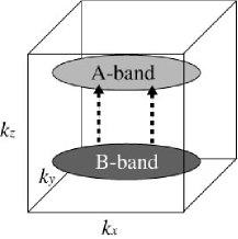
FIG. 1.: Schematic inter-band nesting (arrows) in disconnected Fermi surfaces in 3D.

There, a nesting vector exists across the two bands, and this is envisaged to give the attractive pair-scattering interaction with a nodal plane running in between the two bands. Note that a pair is formed within each band, although the nesting is inter-band. In such a case the gap function should be nodeless within each band, while the gap has opposite signs between the two bands. In this sense the mechanism is an extension of the time-honored Suhl-Kondo mechanism, although there are important differences since here we consider bands originating from multiple orbitals of the same type connected by single electron hopping in order to have appropriate nesting between the disconnected Fermi surfaces, while Suhl-Kondo considers basically the bands originating from different (e.g., s and d) orbitals that interact only via multi electron processes.

For the survey in lattice structures, there are two possible approaches: (i) to find 3D lattice structures whose Fermi surfaces are disconnected, and consider the 3D-version of the mechanism originally proposed for 2D lattices,[3] (ii) stack the 2D lattices already proposed[3, 4, 5, 6] for which $T_{c}\sim O(0.1t)$ has been estimated, and introduce the interlayer hopping, $t_{z}$, to see how the $T_{c}$ behaves as $t_{z}$ is increased. As for the former approach, we have recently studied superconductivity in 3D stacked honeycomb lattice,[9] where the Fermi surface consists of two networks of tubes. However, the networks of tubes have turned out to have such a strong structure that the intra-band as well as inter-band pair-scattering processes contribute to the gap equation, and the resulting gap function has nodes (with $d$-wave symmetry) within each band. Accordingly, the estimated $T_{c}\sim O(0.001t)$ is low, and the stacked honeycomb lattice does not realize the 3D-version of inter-band nesting conceived here.

This has motivated us in the present study to look for models that have more compact and structure-less Fermi surfaces. We have found that a stacked bond-alternating lattice (Fig. 2) has a compact and disconnected Fermi surface (i.e., a pair of ball-like Fermi pockets). We then show for the multiband Hubbard model on this lattice that the inter-band pair-scattering alone is dominant. The estimated $T_{c}$ is $O(0.01t)$, which is the same order of that for the square lattice, and remarkably high for a 3D system.

As for the second approach of stacking the 2D lattices, we have studied the $t_{z}$-dependence of the pairing instability for stacked ladder lattice (Fig. 2). We have found that the $T_{c}\sim O(0.1t)$, found for the single layer, is unexpectedly robust against, or even increases with, $t_{z}$ when $t_{z}$ is not too strong. We have then identified the underlying physics for the favorable condition for the superconductivity on disconnected Fermi surfaces — the system should be quasi-low dimensional, and the peak in the spin susceptibility should be appropriately “blurred”.

So we shall conclude that the idea of raising $T_{c}$ in superconductivity from repulsive electron-electron interaction on disconnected Fermi surfaces can work in 3D lattices if we consider appropriate lattice structures.

II formulation

Here we take the repulsive Hubbard model, a simplest possible model for repulsively interacting electron systems. So the interaction is the ordinary on-site repulsion, $U$, but the lattice has two atoms per unit cell here accompanied by two bands. The Hamiltonian is

$${\cal H} = \sum_{i,j}^{\rm nn}\sum_{\sigma=\uparrow,\downarrow}\sum_{\alpha,\beta={\rm A},{\rm B}}t_{ij}c_{i\sigma}^{\alpha\dagger}c_{j\sigma}^{\beta}$$ (2)

$$+U\sum_{i}\sum_{\alpha={\rm A},{\rm B}}n_{i\uparrow}^{\alpha}n_{i\downarrow}^{\alpha},$$

where $\alpha,\beta$ label A,B sublattices with standard notations otherwise. For the transfer energies $t$, $t_{x_{1}}$, $t_{x_{2}}$ and $t_{y}$ are intra-layer hoppings, while $t_{z}$ the inter-layer (see Fig. 2).

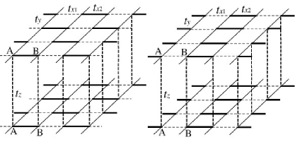
FIG. 2.: A stacked bond-alternating lattice (left panel) and a stacked connected-ladder lattice (right) considered in the present work. Solid lines (dashed lines) indicate stronger (weaker) hopping, and A, B label sublattices.

We employ the FLEX method developed by Bickers et al.[10, 11, 12, 13] In the two-band version of FLEX,[14, 15] Green’s function $G$, self-energy $\Sigma$, susceptibility $\chi$, and the gap function $\phi$ all become $2\times 2$ matrices, such as $G_{\alpha\beta}(k)$, where $\alpha,\beta=$ A,B sublattice, $k\equiv(\mbox{\boldmath$k$},i\omega_{n})$ with $\omega_{n}=(2n-1)\pi T$ being the Matsubara frequency for fermions.

The self-energy is given in the FLEX as

$$\Sigma_{\alpha\beta}(k) = \frac{T}{N}\sum_{k^{\prime}}\left[V_{\alpha\beta}^{\rm ph}(k-k^{\prime})G_{\alpha\beta}(k^{\prime})\right.$$ (4)

$$\left.-V_{\alpha\beta}^{\rm pp}(k-k^{\prime})G_{\beta\alpha}(-k^{\prime})\right],$$

where the particle-hole ($V^{\rm ph}$) and particle-particle ($V^{\rm pp}$) fluctuation-exchange interactions are given as

$$V_{\alpha\beta}^{\rm ph}(q) = \frac{3}{2}U^{2}\!\!\left[\frac{\chi^{{\rm ph}}(q)}{1-U\chi^{{\rm ph}}(q)}\right]_{\alpha\beta}\!\!\!+\frac{1}{2}U^{2}\!\!\left[\frac{\chi^{{\rm ph}}(q)}{1+U\chi^{{\rm ph}}(q)}\right]_{\alpha\beta}\!\!\!\!$$ (6)

$$-U^{2}\chi_{\alpha\beta}^{\rm ph}(q),$$

$$V_{\alpha\beta}^{\rm pp}(q)=U^{2}\left[\frac{\chi^{{\rm pp}}(q)}{1+U\chi^{{\rm pp}}(q)}-\chi^{\rm pp}(q)\right]_{\alpha\beta}\\$$ (7)

with

$$\chi_{\alpha\beta}^{{\rm ph}}(q) = -\frac{T}{N}\sum_{k}G_{\alpha\beta}(k+q)G_{\beta\alpha}(k),$$ (8)

$$\chi_{\alpha\beta}^{{\rm pp}}(q) = \frac{T}{N}\sum_{k}G_{\alpha\beta}(k+q)G_{\alpha\beta}(-k).$$ (9)

Here we denote $q\equiv(\mbox{\boldmath$q$},i\epsilon_{l})$ with $\epsilon_{l}=2\pi lT$ being the Matsubara frequency for bosons, and $N$ the number of $k$-points on a mesh.

Green’s function is related to $\Sigma$ via Dyson’s equation,

$$\left[G(k)^{-1}\right]_{\alpha\beta}=\left[G^{0}(k)^{-1}\right]_{\alpha\beta}-\Sigma_{\alpha\beta}(k),$$ (10)

where $G^{0}$ is the bare Green’s function,

$$G_{\alpha\beta}^{0}(k)=\left[\frac{1}{i\omega_{n}+\mu-\epsilon_{\mbox{\boldmath$k$}}^{0}}\right]_{\alpha\beta}$$ (11)

with $\epsilon_{\mbox{\boldmath$k$}}^{0}$ the energy of a free electron.

The gap function, $\phi$, and $T_{c}$ are obtained from Eliashberg’s equation,

$$\lambda\phi_{\alpha\beta}(k) = -\frac{T}{N}\sum_{k^{\prime}}\sum_{\alpha^{\prime},\beta^{\prime}}$$ (13)

$$V_{\alpha\beta}^{(2)}(k-k^{\prime})G_{\alpha\alpha^{\prime}}(k^{\prime})G_{\beta\beta^{\prime}}(-k^{\prime})\phi_{\alpha^{\prime}\beta^{\prime}}(k^{\prime}),$$

where the (spin-singlet) pairing interaction $V^{(2)}(q)$ is given as

$$V_{\alpha\beta}^{(2)}(q) = \frac{3}{2}U^{2}\!\!\left[\frac{\chi^{{\rm ph}}(q)}{1-U\chi^{{\rm ph}}(q)}\right]_{\alpha\beta}\!\!\!-\frac{1}{2}U^{2}\!\!\left[\frac{\chi^{{\rm ph}}(q)}{1+U\chi^{{\rm ph}}(q)}\right]_{\alpha\beta}$$ (15)

$$+U\delta_{\alpha\beta}.$$

$T_{c}$ is then determined as the temperature at which the largest eigenvalue, $\lambda$, of Eliashberg’s equation becomes unity.

The spin susceptibility in RPA is given by,

$$\chi_{\alpha\beta}(\mbox{\boldmath$k$},0)=\left[\frac{\chi^{{\rm ph}}(\mbox{\boldmath$k$},0)}{1-U\chi^{{\rm ph}}(\mbox{\boldmath$k$},0)}\right]_{\alpha\beta},$$ (16)

may be expressed as diagonalized components,

$$\chi_{\pm}=\frac{\chi_{{\rm AA}}+\chi_{{\rm BB}}}{2}\pm\sqrt{\left[\frac{\chi_{{\rm AA}}-\chi_{{\rm BB}}}{2}\right]^{2}+\left|\chi_{{\rm AB}}\right|^{2}}.$$ (17)

For the two-band FLEX calculation in 3D we take $N=32^{3}$ $k$-point meshes, and the Matsubara frequencies taken as $-(2N_{c}-1)\pi T<\omega_{n}<(2N_{c}-1)\pi T$ with $N_{c}=4096$, which gives converged results.

III result

A Stacked bond-alternating lattice

We have searched for the case where the inter-band nesting is strong with a weak intra-band nesting along the following line. We start from the stacked honeycomb lattice, where the tubular Fermi surface connected along $x-y$ directions has too strong an intra-band nesting as mentioned.[9] One way to make the Fermi surface more compact and structureless is to introduce alternating bonding structures in the $x-y$ plane. For example, if the in-plane bonds along $x$ alternate between weak ones ($t_{x1}$) and strong ones ($t_{x2}$), where the array of strong and weak ones is staggered as we go along $y$ direction. We can then connect the layers with the third-direction hopping $t_{z}$, and we call this the stacked bond-alternating lattice (Fig. 2). We have varied $t_{x_{1}}$ and $t_{z}$ to examine the pairing instability over the region $t_{x_{1}},t_{z}<t_{y}(=1)<t_{x_{2}}$ with a fixed $t_{x_{2}}=2$ for the band filling $n=1.02$. This region has turned out to correspond to the case of compact Fermi pockets. The repulsion is taken to be $U=4$, which is a typical value for strongly correlated systems. Hereafter we take $t_{y}$ as the unit of energy. The Fermi surface and the spin susceptibility for a typical case ($t_{x_{1}}=0.4$, $t_{z}=0.8$) is shown in Fig. 3. We can see that the Fermi surface comprises a pair of compact, ball-like pockets. There exists, as intended, a dominant nesting vector in the stacking direction ($\mbox{\boldmath$k$}=(0,0,\pi)$) across the two pockets, as confirmed from a strong peak in $\chi_{+}(\mbox{\boldmath$k$},0)$ around $\mbox{\boldmath$k$}=(0,0,\pi)$ in Fig. 3.

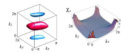
FIG. 3.: (Color) Fermi surface (left panel; blue: bonding band, red: antibonding band) along with $\chi_{+}$ at $k_{z}=\pi$ (right) for the stacked bond-alternating lattice with $U=4$, $n=1.02$, $t_{x_{1}}=0.4$, $t_{x_{2}}=2.0$, $t_{z}=0.8$, $T=0.02$.

Figure 4 shows the result for the dependence of the largest eigenvalue, $\lambda$, of Eliashberg’s equation on the inter-layer hopping, $t_{z}$, for $T=0.02$ and $t_{x_{1}}=0.2$. We can see that $\lambda$ increases with $t_{z}$. This indeed occurs as the two Fermi pockets (displayed in red and blue) begin to be formed and the inter-band nesting across the pockets, that should favor the pairing, develops. For this choice of parameters, however, the superconductivity gives way to antiferromagnetism (whose boundary is identified here to the situation when $1-U\chi^{\rm ph}=0$) around the value of $t_{z}$ at which $\lambda$ reaches unity. Nevertheless we are on the right track in that the gap function is, as intended, nodeless (gapful) in each band while changes sign across the two bands.

So we should next tune the shape of the two Fermi pockets. This can be achieved by varying the weak hopping, $t_{x_{1}}$, in the bond-alternating system. As seen in Fig. 5, the Fermi surface for each band remains to be two balls throughout, but they become more compact as $t_{x_{1}}$ is increased. If we turn to $\lambda$ in the figure for a fixed $t_{z}=0.8$ with $T=0.02$, $\lambda$ indeed reaches unity well before the antiferromagnetism sets in. In the case of $t_{x1}=0$ (with a low $T_{c}$), the gap function has a nodal plane as shown by green sheet in Fig. 5, which should be due to the main $(0,0,\pi)$ pair scattering in large antibonding band Fermi surface favor node to change the sign across the scattering.

So we conclude for the bond-alternating model that, although disconnected Fermi surfaces are favorable for the inter-band pairing, the Fermi pockets have to be compact so that the intra-band pair-scattering is suppressed and the gap function for each band becomes nodeless.

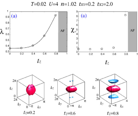
FIG. 4.: (Color) The largest eigenvalue, $\lambda$ (top left), of Eliashberg’s equation and the peak value of spin susceptibility $\chi_{+}$ (top right, with the gray region indicating the antiferromagnetic phase) as a function of the inter-layer hopping $t_{z}$, along with the Fermi surface (bottom) for selected values of $t_{z}$ for $U=4$, $n=1.02$, $t_{x_{1}}=0.2$, $t_{x_{2}}=2.0$, $T=0.02$ for the stacked bond-alternating lattice.

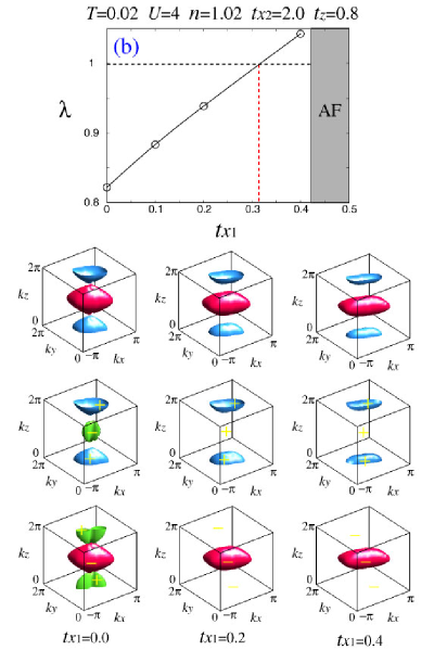
FIG. 5.: (Color) A plot similar to Fig. 4 (top two rows) when we vary the weak hopping, $t_{x_{1}}$, in the stacked bond-alternating lattice with fixed $t_{x_{2}}=2.0$, $t_{z}=0.8$ for $U=4$, $n=1.02$, and $T=0.02$. We depict the gap function with its sign indicated on the Fermi surface for the bonding (second from bottom row) and antibonding (bottom) bands, respectively, where nodal planes are shown by green sheets.

We have then scanned the $t_{x_{1}}-t_{z}$ parameter plane to optimize the values of $t_{x_{1}}$ and $t_{z}$, and found that $\lambda$ takes its maximum at $t_{x_{1}}=0.4$, $t_{z}=0.8$. In Fig. 6, temperature dependence of $\lambda$ for the optimized case is plotted. We can see that $T_{c}\sim 0.02t_{y}$, which is remarkably high (i.e., $\simeq 2\times 10^{-3}\times$ the bandwidth with the bandwidth $\simeq 12t_{y}$) for a 3D system (where usually $T_{c}\sim 10^{-4}\times$ bandwidth at most as estimated for the simple cubic lattice[2]).

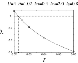
FIG. 6.: $\lambda$ as a function of $T$ for the optimized $t_{x_{1}}=0.4$ and $t_{z}=0.8$ for the stacked bond-alternating lattice with $U=4$, $n=1.02$, $t_{x_{2}}=2.0$, and $T=0.02$.

B Stacked connected-ladder lattice

Let us move on to the stacked connected-ladder lattice (right panel in Fig.2). In this subsection, we fix $n=1.05,U=4.0,t_{x_{2}}=1.6,t_{y}=1({\rm unit})$. This value of $t_{x_{2}}$ turns out to give the highest $T_{c}$ for $U=4$. In 2D Kuroki and Arita[3] have shown that a larger $U=8$ gives a higher $T_{c}$, but in the present case of 3D the tendency toward AF is stronger, so that we take a weaker $U=4$ as in the previous section.

Figure 7 shows $\lambda$ and $\chi_{+}$ as a function of the inter-layer hopping $t_{z}$ for a fixed $t_{x1}=0.1$ with $T=0.06$. We can see that $\lambda$ is as large as, or even greater than, in 2D ($t_{z}=0$) up to $t_{z}<0.3$. For smaller $t_{z}<0.2$ the Fermi surface consists of only one band (two panels at bottom left in Fig.7). In this case the inter-band nesting is weak, as seen from a small $\chi_{+}$ (top right in Fig.7). When $t_{z}>0.3\gg t_{x1}$, the system becomes quasi-2D along the $yz$ plane, and a nesting in the direction of $(0,\pi,\pi)$ evolves (as evident from the shape of the Fermi cylinders that change their direction from $\parallel z$ to $\parallel x$). While $\chi_{+}$ monotonically increases with $t_{z}$ throughout, superconductivity is most favored ($\lambda\simeq 1$ in between ($t_{z}\simeq 0.2$).

The resultant $T_{c}\simeq 0.06$ in the 3D system is $T_{c}\simeq 8\times 10^{-3}\times$ bandwidth (with the bandwidth $\simeq 8t_{y}$), which is even higher than in the above bond-alternating lattice, and almost an order of magnitude higher than the ordinary 3D case of $\simeq 10^{-4}\times$ bandwidth. This shows that the superconductivity in the disconnected Fermi surface proposed in Ref.[3] for 2D is robust against introduction of the third-direction hopping.

C Condition favoring the pairing on disconnected Fermi surfaces

The peak in $T_{c}$ at a nonzero $t_{z}$ (rather than at $t_{z}=0$) seen above is surprising. This is particularly puzzling since the spin susceptibility increases monotonically with $t_{z}$, which implies that a good nesting per se does not necessarily favor the pairing. We then want to pin-point the physical reason why superconductivity is degraded although $\chi_{+}$ increases in the region of $t_{z}>0.3$.

To elaborate the question let us look at another, similar phenomenon when we increase the in-plane, inter-ladder hopping, $t_{x_{1}}$, with a fixed $t_{z}=0.2$ in Fig. 8. There, we can see that, although the nesting, in the direction of $(0,\pi,\pi)$, evolves with $t_{x_{1}}$ as shown from both the shape of the Fermi surface and the value of $\chi_{+}$ in Fig. 8, $\lambda$ decreases as $\chi_{+}$ increases, which provides another example of the degraded superconductivity in the evolution of the nesting.

We can conceive several reasons as follows. As we have mentioned, the increase of $t_{z}$ or $t_{x1}$ raises the dimensionality of the anisotropic system to 3D. This should degrade superconductivity in two ways. First one is just the mechanism revealed by Arita et al. in ref.[2], where higher the dimension smaller the phase volume fraction for the pairing interaction. Secondly, when $E_{F}$ is close to band edges, the density of states there tends to be smaller for higher dimensions. To see that this is indeed the case, we have examined in Figs.10,11 the regions in $k$-space in which

$\displaystyle\mu-\delta\mu<\epsilon^{0}+{\rm Re}\Sigma<\mu+\delta\mu,$

which we will refer to as the “thickness” of the Fermi surface. Bulkier the thickness larger the density of states, but we specifically take the energy window $\delta\mu$ as the energy interval over which ${\rm Im}\chi_{+}({\mbox{\boldmath$k$}_{\rm max}},\omega)$ (with $\mbox{\boldmath$k$}_{\rm max}$ being the momentum that gives the peak in $\chi_{+}$), displayed in Fig.9, is significant. In other words, $\delta\mu$ is the energy scale of the spin fluctuations that mediate the pairing. As seen in Figs. 10,11, respectively, increased $t_{z}$ or $t_{x1}$ makes the Fermi surface “thinner” although the Fermi surface itself is large. The situation is shown schematically in Fig.12

Another factor governing superconductivity can also be identified from Figs.10,11. Namely, since we are here dealing with small (or vanishing) Fermi surfaces, the spin susceptibility is governed not by the shape of the Fermi surface itself, but by the thickened Fermi surface. The thin Fermi surfaces for smaller $t_{z}$ or $t_{x1}$ then make the nesting sharper and the peak in $\chi_{+}$ becomes narrower. This also acts to degrade superconductivity, since the spin susceptibility has to be appropriately “blurred” in order to make the spin fluctuation usable over a large phase space for pair scattering.

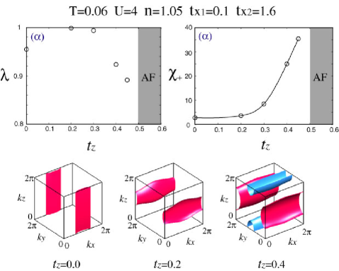
FIG. 7.: (Color) $\lambda$ (top left) and $\chi_{+}$ (top right) as a function of the inter-layer hopping $t_{z}$ along with the Fermi surface for the stacked connected-ladder lattice with selected values of $t_{z}$ (as indicated at the bottom) for the stacked-ladder lattice for $U=4$, $n=1.05$, $t_{x_{1}}=0.1$, $t_{x_{2}}=1.6$, $T=0.06$.

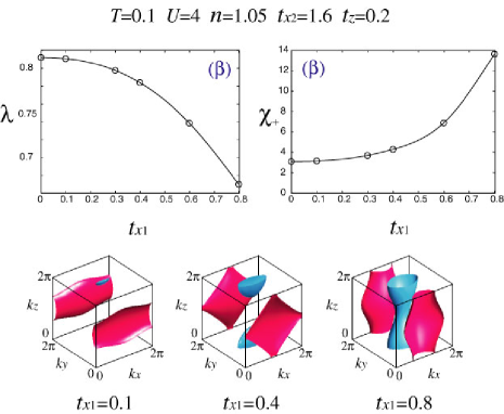
FIG. 8.: A plot similar to Fig. 7 for the stacked connected-ladder lattice when the weak hopping, $t_{x1}$, is varied as indicated at the bottom for a fixed $t_{z}=0.2$ with $U=4$, $n=1.05$, $t_{x_{2}}=1.6$, and $T=0.1$.

FIG. 9.: ${\rm Im}\chi_{+}(\mbox{\boldmath$k$}_{\rm max},\omega)$ (normalized by its maximum value), where $\mbox{\boldmath$k$}_{\rm max}=(0,\pi,\pi)$, as a function of $\omega$ for $T=0.06,U=4,n=1.05,t_{x_{1}}=0.1,t_{x_{2}}=1.6,t_{z}=0.2$ for the stacked connected-ladder lattice.

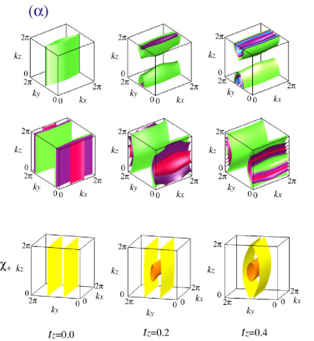
FIG. 10.: (Color) Top: The regions in the $k$-space bounded by $\mu-\delta\mu<\epsilon^{0}+{\rm Re}\Sigma<\mu+\delta\mu$ with $\delta\mu=0.5$(purple), $1$(green), along with the Fermi surface (blue: the bonding band which is only visible in the right row, red: the anti-bonding band) on which the region of $\epsilon^{0}+{\rm Re}\,\Sigma=\mu$ is displayed for the stacked connected-ladder lattice with selected values of the inter-layer hopping $t_{z}$ as in Fig.7 as indicated at the bottom. Bottom: $k$-space contours (orange: $\chi_{+}=3$, yellow: $\chi_{+}=1$) of the spin susceptibility.

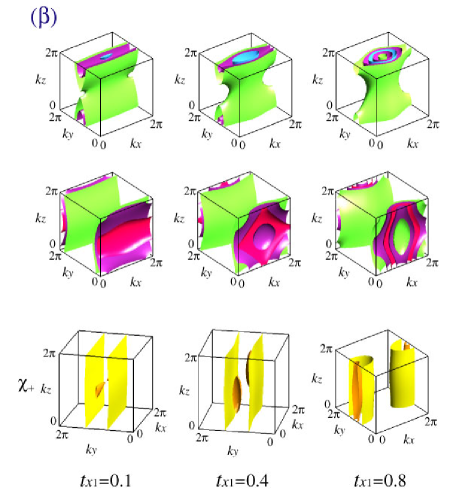
FIG. 11.: (Color) A plot similar to Fig. 10 for the stacked connected-ladder lattice when the weak hopping, $t_{x_{1}}$, is varied as in Fig.8 as indicated at the bottom.

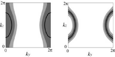
FIG. 12.: The schematic ”thickness” of Fermi surface at $k_{x}=\pi$. The light gray and dark gray regions represent $0.5<|\epsilon^{0}-\mu+{\rm Re}\Sigma|<1$ and $0<|\epsilon^{0}-\mu+{\rm Re}\Sigma|<0.5$, respectively, and Fermi surfaces are shown by black lines. The left panel has larger gray (active) region than the right.

IV Conclusion

We have studied how the pairing with higher $T_{c}$ in disconnected Fermi surfaces can be realized in three-dimensional systems. Our first proposal of the stacked bond-alternating lattice has a pair of ball-like Fermi pockets with a dominant inter-band nesting vector and antiferromagnetic spin fluctuations, which is a genuinely 3D model in that the interlayer hopping $t_{z}$ promotes the inter-band pairing. $T_{c}$ estimated from Eliashberg’s equation shows that $T_{c}\sim 10^{-3}$ times the bandwidth ($\sim O(0.01t)$), which is as high as that for the single-band Hubbard model on the square lattice, and remarkably high for 3D system.

Our second model of the stacked layers each having a disconnected Fermi-surface in 2D originally proposed by Kuroki and Arita[3] is shown to have a high $T_{c}$ that is robust against the introduction of the inter-layer hopping, although the hopping degrades the 2D nesting. The estimated $T_{c}\sim$ several times $10^{-3}\times$ bandwidth ($=$ several times $O(0.01t)$) is even higher than the first model.

From these we have then identified the right conditions for higher $T_{c}$ in the disconnected Fermi surface: the system should be quasi-low dimensional, and the peak in the spin susceptibility should be not too sharp but “blurred”. So the message here is that 3D materials with considerably high $T_{c}$ can be expected if we consider appropriate lattice structures.

V Acknowledgements

Numerical calculations were performed at the Computer Center and the ISSP Supercomputer Center of University of Tokyo. This study was in part supported by a Grant-in-aid for scientific research from the Ministry of Education of Japan.

REFERENCES

- [1] J. G. Bednortz and K. A. Müller, Z. Phys. B 64, 189 (1986).
- [2] R. Arita, K. Kuroki, and H. Aoki, Phys. Rev. B 60, 14585 (1999); J. Phys. Soc. Jpn. 69, 1181 (2000).
- [3] K. Kuroki and R. Arita, Phys. Rev. B 64, 024501 (2001).
- [4] T. Kimura, H. Tamura, K. Kuroki, K. Shiraishi, H. Takayanagi, and R. Arita, Phys. Rev. B 68, 132508 (2002).
- [5] T. Kimura, Y. Zenitani, K. Kuroki, R. Arita, and H. Aoki, Phys. Rev. B 66, 212505 (2002).
- [6] T. Kimura, K. Kuroki, and R. Arita, Phys. Rev. B 66, 132508 (2002).
- [7] P. Monthoux and G. G. Lonzarich, Phys. Rev. B 59, 14598 (1999).
- [8] P.G. Pagliuso, R. Movshovich, A.D. Bianchi, M. Nicklas, N.O. Moreno, J.D. Thompson, M.F. Hundley, J.L. Sarrao, and Z. Fisk, Physica B 312, 129 (2002).
- [9] S. Onari, K. Kuroki, R. Arita, and H. Aoki, Phys. Rev. B 65, 184525 (2002).
- [10] N. E. Bickers, D. J. Scalapino, and S. R. White, Phys. Rev. Lett. 62, 961 (1989).
- [11] N. E. Bickers and D. J. Scalapino, Ann. Phys. (N.Y.) 193, 206 (1989).
- [12] T. Dahm and L. Tewodt, Phys. Rev. B 52, 1297 (1995).
- [13] M. Langer, J. Schmalian, S. Grabowski, and K. H. Bennemann, Phys. Rev. Lett. 75, 4508 (1995).
- [14] S. Koikegami, S. Fujimoto, and K. Yamada, J. Phys. Soc. Jpn. 66, 1438 (1997).
- [15] H. Kontani and K. Ueda, Phys. Rev. Lett. 80, 5619 (1998).