Corridors of barchan dunes: stability and size selection.

Abstract

Barchans are crescentic dunes propagating on a solid ground. They form dune fields in the shape of elongated corridors in which the size and spacing between dunes are rather well selected. We show that even very realistic models for solitary dunes do not reproduce these corridors. Instead, two instabilities take place. First, barchans receive a sand flux at their back proportional to their width while the sand escapes only from their horns. Large dunes proportionally capture more than they loose sand, while the situation is reversed for small ones: therefore, solitary dunes cannot remain in a steady state. Second, the propagation speed of dunes decreases with the size of the dune: this leads – through the collision process – to a coarsening of barchan fields. We show that these phenomena are not specific to the model, but result from general and robust mechanisms. The length scales needed for these instabilities to develop are derived and discussed. They turn out to be much smaller than the dune field length. As a conclusion, there should exist further – yet unknown – mechanisms regulating and selecting the size of dunes.

Since the pioneering work of Bagnold B41 , sand dunes have become an object of research for physicists. Basically, the morphogenesis and the dynamics of dunes result from the interaction between the wind, which transports sand grains and thus modifies the shape of the dune, and the dune topography which in turn controls the air flow. A lot of works have been devoted to the study of the mechanisms at the scale of the grain O64 ; H77 ; S85 ; JS86 ; AH88 ; AH91 ; ASW91 ; S91 ; WMR91 ; RM91 ; NHB93 ; IR94 ; RIR96 ; RVB00 ; SKH01 ; A03 and at the scale of single dune B10 ; F59 ; C64 ; LS64 ; H67 ; N66 ; H87 ; S90 ; HH98 ; SRPH00 ; ACD02b ; HDA02 ; M88 ; ZJ87 ; JH75 ; HMGP78 ; JZ85 ; WG86 ; HLR88 ; WHCWWLC91 ; W95 ; BAD99 ; KSH01 ; S01 . The interested reader should refer to a previous paper ACD02a for a review of these works. Our aim is to focus here on dune fields and to show that most of the problems at this scale are still open or even ill-posed.

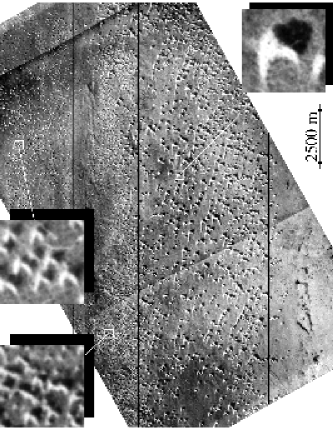
Figure 1: Aerial photograph showing part of the barchan field extending between Tarfaya, Laayoune and Sidi Aghfinir in southern Morocco, former Spanish Sahara. The trade winds, dominant in the region, blow from the north (from the top of the photograph). Several corridors are visible in which the size of barchans and their density is almost uniform. As confirmed by the three zooms, the size of dunes is different from one corridor to another.

The most documented type of dune, the barchan , is a crescentic shaped dune, horns downwind, propagating on a solid ground. In the general picture emerging from the literature, barchans are thought as solitary waves propagating downwind without changing their shape and weakly coupled to their neighborhood. For instance, most of the field observations concern geometric properties (morphologic relationships) and kinematic properties (propagation speed). This essentially static description probably results from the fact that barchans do not change a lot at the timescale of one field mission.

As shown on figure 1, barchans usually do not live isolated but belong to rather large fields LL69 . Even though they do not form a regular pattern, it is obvious that the average spacing is a few times their size, and that they form long corridors of quite uniformly sized dunes. Observing the right part of figure 1, the barchans have almost all the same size ($6~{}m$ to $12~{}m$ high, $60~{}m$ to $120~{}m$ long and wide). Observing now the left part of figure 1, the barchans are all much smaller ($1.5~{}m$ to $3~{}m$ high, $15~{}m$ to $30~{}m$ long and wide) and a small band can be distinguished, in which the density of dunes becomes very small. Globally, five corridors stretched in the direction of the dominant wind can be distinguished: from right to left, no dune, large dunes, small dunes, no dune and small dunes again. Figure 1 shows only $17~{}km$ of the barchan field. Direct observations show that these five corridors persist in a coherent manner over hundreds of kilometers along the dominant wind direction.

The content of this paper is perhaps a bit unusual as we will mostly present negative results. Indeed, we will show that none of the dune models HMGP78 ; JZ85 ; WG86 ; HLR88 ; WHCWWLC91 ; W95 ; BAD99 ; KSH01 ; S01 , nor the coarse grained field simulation LSHK02 are able at present to reproduce satisfactorily the selection of size and the formation of corridors.

More precisely, we shall first address the stability of solitary dunes, and conclude that, given reasonable orders of magnitude for dune sizes and velocities, barchans which are considered as “marginally unstable” by other authors S01 would in fact have the time to develop their instability over a length much smaller than that of the corridor they belong to. As a consequence, isolated dunes must be considered as truly unstable objects. Furthermore, the origin of this instability is rather general and model independent, as it can be understood from the analysis of the output sand flux as a function of the dune size.

One can wonder whether interactions via collisions between dunes can modify the dynamics and the stability of dunes. In a recent paper Lima et al. LSHK02 have investigated the dynamics of a field and have claimed to get realistic barchan corridors. However, they made use of numerical simulations into which individual dunes are stable objects of almost equal size ($6\%$ of polydispersity). They consequently obtained a nearly homogeneous field composed of dunes whose width is that of those injected at the upwind boundary. We show here that the actual case of individually unstable dunes leads by contrast to an efficient coarsening of the barchan field.

The paper is organized as follows. In order to get a good idea of the mechanisms leading to these two instabilities, we first derive a 3D generalization of the $\mbox{{C}}_{\mbox{{c}}}^{\mbox{{c}}}$ model previously used to study 2D dunes ACD02b . We then show that the two instabilities predicted by the $\mbox{{C}}_{\mbox{{c}}}^{\mbox{{c}}}$ model are in fact very general and we will derive in a more general framework the time and length scales over which they develop. Turning to field observations, we will conclude that the formation of nearly uniform barchan corridors is an open problem: there should exist further mechanisms, not presently known and may be related to more complicated and unsteady effects such as storms or change of wind direction, to regulate the dune size.

I Barchan modeling. The $\mbox{{C}}_{\mbox{{c}}}^{\mbox{{c}}}$ model

We start here with the state of the art concerning the modeling of dunes by Saint-Venant like equations. First, the mechanisms of transport at the scale of the grain O64 ; S85 ; JS86 ; AH88 ; AH91 ; ASW91 ; S91 ; WMR91 ; RM91 ; NHB93 ; IR94 ; RIR96 ; RVB00 ; SKH01 ; A03 ; ACD02a determine at the macroscopic scale – at the scale of the dune – the maximum quantity of sand that a wind of a given strength can transport. As a matter of fact, when the wind blows over a flat sand bed, the sand flux increases and saturates to its maximum value $Q$ after a typical length $L$ called the saturation length B41 ; SKH01 ; ACD02b ; HDA02 . This length determines the size of the smallest propagative dune.

The other part of the problem is to compute the turbulent flow around a huge sand pile of arbitrary shape M88 ; ZJ87 . Since the Navier-Stokes equations are far too complicated to be completely solved, people have derived simplified descriptions of the turbulent boundary layer JH75 ; HMGP78 ; JZ85 ; WG86 ; HLR88 ; WHCWWLC91 ; W95 ; BAD99 ; KSH01 ; S01 . The first step initiated by Jackson, Hunt et al. has been to derive an explicit expression of the basal shear stress in the limit of a very flat hill. Kroy et al. KSH01 ; S01 have shown that this expression can be simplified without loosing any important physical effect. In particular, it keeps the non-local feature of the velocity field: the wind speed at a given place depends on the whole shape of the dune.

Being a linear expansion, this approach can not account for boundary layer separation and in particular for the recirculation bubble that occurs behind dunes. Following Zeman and Jensen ZJ87 and later Kroy et al., the Jackson and Hunt formula is in fact applied to an envelope of the dune constituted by the dune profile prolonged by the separation surface.

As already stated in one of our previous papers ACD02b , we proposed to name $\mbox{{C}}_{\mbox{{c}}}^{\mbox{{c}}}$ the class of models which describe the dynamics of dunes in terms of the dune profile $h$ and the sand flux $q$, and which include (i) the mass conservation, (ii) the progressive saturation of sand transport and (iii) the feedback of the topography on the sand erosion/deposition processes. We chose this fancy name in reference to the spatial organization of the dunes which propagate like the flight of wild ducks and geese.

I.1 2D and 3D main equations

Let us start with a quick recall of the set of 2D $\mbox{{C}}_{\mbox{{c}}}^{\mbox{{c}}}$ equations that we already introduced in ACD02b . Let $x$ denote the axis oriented along the wind direction, and $t$ the time. The continuity equation which ensures mass conservation simply reads

$$\partial_{t}h+\partial_{x}q=0.$$ (1)

Note that $q(x,t)$ denotes the integrated volumic sand flux, i.e. the volume of sand that crosses at time $t$ the position $x$ per unit time. The saturation process is modeled by the following charge equation

$$\partial_{x}q=\frac{q_{sat}-q}{L}.$$ (2)

It is enough to incorporate the fact that the sand flux follows the saturated flux $q_{sat}$ with a spatial lag $L$. It is a linearized version of the charge equation proposed by Sauermann et al. SKH01 .

The saturated flux $q_{sat}$ is a growing function of the shear stress. This shear stress can be related to the dune profile $h$ by the modified Jackson and Hunt expression. Since this expression comes from a linear expansion, we can directly relate $q_{sat}$ to $h$ by:

$$\frac{q_{sat}(x)}{Q}=1+A\int\!\!\frac{d\chi}{\pi\chi}\,\partial_{x}h_{e}(x-\chi)+B\,\partial_{x}h_{e}(x),$$ (3)

where $Q$ is the saturated flux on a flat bed and $h_{e}$ the envelope prolonging the dune on the lee side (see Appendix and KSH01 ; ACD02b for the details of construction). The last term takes into account slope effects, while the convolution term encodes global curvature ones. The only relevant length scale is the saturation length $L$ of the sand flux. The other relevant physical parameter is the saturated sand flux on a flat bed $Q$. All the lengths are calculated in units of $L$, time in units of $Q/L^{2}$, and fluxes in unit of $Q$. $A$ and $B$ could in principle be predicted by the Jackson and Hunt analysis but we rather take them as two tunable phenomenological constants.

In three dimensions, equations are very similar, albeit slightly different. In order to express the total sand flux (which is now a 2D vector), we need to distinguish saltons and reptons H03 . The reason is that in contrast to the saltons, which follow the wind, the motion of the reptons is sensitive to the local slope H77 . Because the reptons are dislodged by the saltons, we assume that their fluxes are proportional A03 , so that the total flux can be written as the sum of two terms, one along the wind direction $\vec{x}$ and the other along the steepest slope H77 :

$${\vec{q}}_{tot}=q\,\vec{x}-Dq\,\vec{\nabla}h.$$ (4)

The continuity equation then takes its generalized form

$$\partial_{t}h+\vec{\nabla}\!\cdot{\vec{q}}_{tot}=0.$$ (5)

The down slope flux of reptons acts as a diffusive process. The diffusion coefficient is proportional to $q$ so that no new scale is introduced – $D$ is a dimensionless parameter. This diffusion term introduces a non-linearity that has a slight effect only: almost the same dynamics is obtained if a constant diffusion coefficient is used instead. Equations (2) and (3) can be solved independently in each slice along $x$.

In summary, the $\mbox{{C}}_{\mbox{{c}}}^{\mbox{{c}}}$ model considered here includes in a simple way all the known dynamical mechanisms for interactions between the dune shape, the wind and the sand transport.

I.2 Propagative solutions of the $\mbox{{C}}_{\mbox{{c}}}^{\mbox{{c}}}$ model.

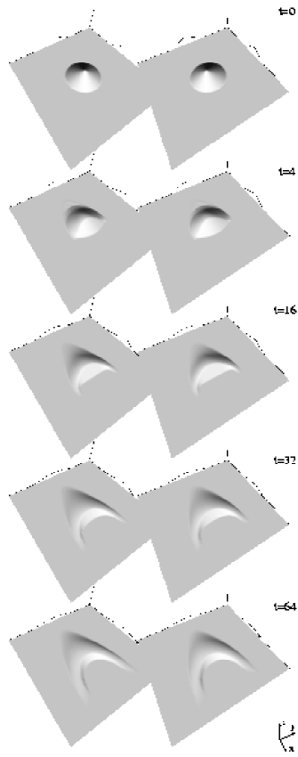
Figure 2: Evolution from a conical sand pile to a steady propagative barchan computed from the $\mbox{{C}}_{\mbox{{c}}}^{\mbox{{c}}}$ model. To obtain this steady solution the output flux is re-injected homogeneously at the upwind boundary. Times are given in units of $L^{2}/Q$. Stereoscopic view: a) place the figure at $\sim 60~{}cm$ from your eyes b) focus behind the sheet, at infinity (you should see three dunes) c) focus on the middle dune and relax d) you should see the shape in 3D.

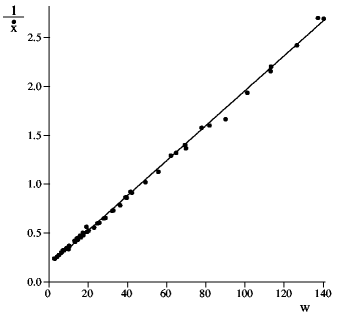
Figure 3: Relationship between the inverse velocity $1/\dot{x}$ and the width $w$ for barchans in the steady state. The line corresponds to the best fit by a Bagnold-like relation of the form $\dot{x}=aQ/(w+w_{c})$. It gives $a=56$ and $w_{c}=9.5$.

In a previous paper ACD02b , we have studied in details steady propagative solutions in the 2D case. They also apply to transverse dunes, i.e. invariant in the $y$ direction. We will now focus on three dimensional solitary dunes computed with the $\mbox{{C}}_{\mbox{{c}}}^{\mbox{{c}}}$ model presented in the latter section. The details of the integration algorithm and the numerical choice of the different parameters can be found in the Appendix and a more detailed discussion about the influence of the diffusion parameter is discussed in H03 . Figure 2 shows in stereoscopic views the time evolution of an initial conical sand pile ($t=0$). Horns quickly develop ($t=16$ and $t=32$) and a steady barchan shape is reached after typically $t=50$. Note that the propagation of the dune is not shown on figure 2: the center of mass of the dune is always kept at the center of the computation box.

The original $\mbox{{C}}_{\mbox{{c}}}^{\mbox{{c}}}$ model proposed by Kroy, Sauermann et al. KSH01 ; S01 was the first of a long series of models in which a steady solitary solution could be exhibited, with all the few known properties of barchans. In particular, the dunes present a nice crescentic shape with a length, a width, a height and a horn size that are related to each others by linear relationships. They propagate downwind with a velocity inversely proportional to their size, as observed on the field. These properties are robust inside the class of modeling, since we get the same results with the simplified version that we use here. We will only show in the following two of these properties, important for the stability discussion, namely the velocity and the volume as functions of the dune size.

Since they are linearly related one to the others, all the dimensions are equivalent to parameterize the dune size. We choose the width $w$ as it is directly involved in the expression of the sand flux at the rear of the dune. Figure 3 shows the inverse of the propagation velocity of the dune as a function of $w$. The velocity decreases as the inverse of the size:

$$\dot{x}\sim\frac{aQ}{w+w_{c}}\,.$$ (6)

Preliminary fields measurements of the displacement of the dunes shown on figure 1 over $27$ years have given $aQ=3700~{}m^{2}/year$ and $w_{c}=33~{}m$. The transverse velocity $\dot{y}$ is found to be null, as lateral inhomogeneities of the sand flux are unable to move dunes sideways LSHK02 . The volume of $V$ is plotted on figure 4. This relation is well fitted by:

$$V=bw^{2}(w+w_{v}),$$ (7)

where the numerical coefficients are $b\sim 0.011$ and $w_{v}\sim 22.9$. This value roughly corresponds to the volume of a half pyramid, with a height $h\sim 0.1\,w$ and a width $w$ which gives a volume $V\sim w^{3}/60$. One can observe that barchan dune are not self similar object: the deviation observed for small dunes is related to the change of shape due to the existence of a characteristic length $L$.

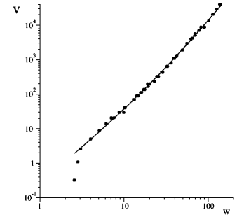
Figure 4: Relationship between the volume $V$ and the width $w$ of solitary barchans. Note the log-log scales. The solid line corresponds to the best fit by the relation $V=bw^{2}(w+w_{v})$. It gives $b=0.011$ and $w_{v}=22.9$.

I.3 Instabilities

The choice of the boundary conditions is absolutely crucial: to get stationary solutions, the sand escaping from the dune and reaching the downwind boundary is uniformly re-injected at the upwind one. Obviously, this ensures the overall mass conservation. Doing so, the simulation converges to a barchan of well defined shape of width $w_{\infty}$ with a corresponding sand flux $q_{\infty}$.

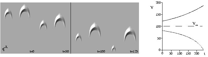
Figure 5: Origin of the flux instability. Two dunes are submitted to a given flux, which is not the equilibrium sand flux for both dunes. The small dune (dotted line) is then under supplied an can only shrink. On the contrary, the bigger dune (solid line) receive too much sand and grows. The evolution of their volume $V$ is depicted on the right. Eventually, the small one disappears.

However, under natural conditions, the input flux $q$ is imposed by the upwind dunes. We thus also performed simulations with a given and constant incoming flux. Figure 5 shows the evolution of two dunes of different sizes under an imposed constant input flux. One is a bit larger than the steady dune corresponding to the imposed flux, and the other is slightly smaller. It can be observed that none of these two initial conditions lead to a steady propagative dune: the small one shrinks and eventually disappears while the big one grows for ever. The steady solution obtained with the re-injection of the output flux is therefore unstable.

If solitary dunes are unstable, it is still possible that the interaction between dunes could stabilize the whole field. It is not what happened in the $\mbox{{C}}_{\mbox{{c}}}^{\mbox{{c}}}$ model. Instead, an efficient coarsening takes place as shown by Sauermann in the chapter $8$ of S01 .

As a first conclusion, the $\mbox{{C}}_{\mbox{{c}}}^{\mbox{{c}}}$ model predicts that solitary barchans and barchan fields are unstable in the case of a permanent wind. We will see below that these two instabilities are generic and not due to some particularity of the modeling. In particular, they can be also observed with the more complicated equations of Kroy, Sauermann et al. who deal with a non-linear charge equation and take explicitly into account the existence of a shear stress threshold to get erosion.

Therefore, we can wonder what are the dynamical mechanisms responsible for these instabilities. Would they have time/length to develop in an actual barchan field? Seeking answers to these questions, we will now investigate the two instabilities in a more general framework. As a first step, we will investigate the time and length scales associated to the evolution of barchan dunes.

II Time and length scales

Three different time scales govern the dynamics of dunes: a very short one for aerodynamic processes (i.e. the grain transport), the turnover time for the dune motion, and a much larger time scale involved in the evolution of the dune volume and shape under small perturbations of the wind properties.

II.1 Turnover time

The dune memory time is usually defined as the time needed to propagate over its own length. Since the length and the width of the dune are almost equal – this is only a good approximation for steady dunes – we will use here the turnover time:

$$\tau_{t}=\frac{w}{\dot{x}}.$$ (8)

In the geological community, the turnover time is believed to be the time after which the dune looses the memory of its shape. The idea is that a grain remains static inside the dune during a cycle of typical time $\tau_{t}$: it then reappears at the surface and is dragged by the wind to the other side of the dune. In other words, after $\tau_{t}$ all the grains composing a dune have moved, and the internal structure of the dune has been renewed. But this does not preclude memory of the dune shape at times larger than $\tau_{t}$, and one can wonder whether $\tau_{t}$ is the internal relaxation time scale to reach its equilibrium shape.

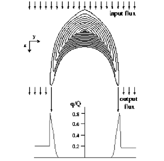
Figure 6: Top: three dimensional shape of a barchan dune obtained with the $\mbox{{C}}_{\mbox{{c}}}^{\mbox{{c}}}$ model, with semi-periodic boundary conditions to ensure the mass conservation. Bottom: profile of the resulting output sand flux. The sand loss is localized at the tips of the horns. There, the flux is almost saturated: $q\sim Q$.

The scaling (6) of the propagation speed involves the cut-off length scale $w_{c}$, which can be measured by extrapolating the curve of 3 to zero. Note that the existence of a characteristic length scale also appears in the dune morphology SRPH00 ; KSH01 ; S01 ; ACD02b . In the following, we will assume that the barchans are sufficiently large to be considered in the asymptotic regime. We checked that introducing cuts-off $w_{c}$ or $w_{v}$ to capture the shape of curves like that of figures 3 or 4 in the region of small $w$ does not change qualitatively the results. In the following we then take $w_{c}=0$ and $w_{v}=0$ for simplicity. Under this assumption, using the expression (6) of the propagation speed, the turnover time reads:

$$\tau_{t}=\frac{w^{2}}{aQ}.$$ (9)

Of course, the length scale $\lambda_{t}$ associated with the turnover time is the size of the dune itself:

$$\lambda_{t}=w.$$ (10)

II.2 Relaxation time

Let us consider, now, a single barchan dune submitted to a uniform sand flux. The evolution of its volume is governed by the balance of incoming $\phi_{in}$ and escaping $\phi_{out}$ sand volumes per unit time:

$$\dot{V}=\phi_{in}-\phi_{out}.$$ (11)

$\phi_{in}$ is directly related to the local flux $q$ upwind the dune, defined as the volume of sand that crosses a horizontal unit length line along the transverse direction $y$ per unit time. Assuming that this flux $q$ is homogeneous, the dune receives an amount of sand simply proportional to its width $w$:

$$\phi_{in}=qw.$$ (12)

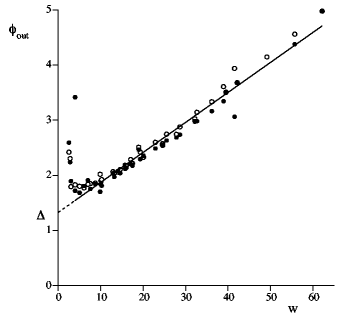
Figure 7: Output flux $\phi_{out}$ as a function of the barchan width $w$ for the equilibrium input flux (white circles) and for a null input flux (black circles). $\phi_{out}$ is not simply proportional to $w$ and does not vanish at small size. As a consequence, the sand loss is proportionally smaller for a large dune than for a small one. The straight line corresponds to the best fit by a function of the form $\phi_{out}=Q(\Delta+\alpha w)$. It gives $\Delta=1.33$ and $\alpha=0.05$.

The loss of sand $\phi_{out}$ is not simply proportional to $w$ because the output flux is not homogeneous. Figure 6 shows the flux in a cross-section immediately behind the dune. One can see that the sand escapes only from the tip of the horns, where there is no more avalanche slip face. As a matter of fact, the recirculation induced behind the slip face traps all the sand blowing over the crest. We computed in the model the output flux $\phi_{out}$ as a function of the dune width $w$ (figure 7). Within a good approximation it grows linearly with $w$:

$$\phi_{out}\sim Q(\Delta+\alpha w).$$ (13)

For the set of parameters chosen, the best fit gives $\alpha=0.05$ and $\Delta=1.33~{}L$. Note that the discrepancy of $\phi_{out}$ with the linear variation for small dunes can be understood by the progressive disappearance of the slip face (domes), leading to a massive loss of sand.

It can be observed from figure 6 that $q$ is almost saturated in the horns. The ratio $\phi_{out}/Q$ then has a geometrical interpretation as it gives an estimate of the size of the horn tips. Therefore, in the $\mbox{{C}}_{\mbox{{c}}}^{\mbox{{c}}}$ model, the horn size is not proportional to the dune width, but grows as $\Delta+\alpha w$. This is consistent with the observations made by Sauermann et al. in southern Morocco: they claim that, at least for symmetric solitary dunes, the slip face is proportionally larger for large dunes than for small ones, i.e. that the ratio of the horns width to the barchan width decreases with $w$.

With these two expressions for the input and output volume rates, the volume balance reads:

$$\dot{V}=qw-Q(\alpha w+\Delta).$$ (14)

If we call $w_{\infty}$ and $q_{\infty}$ the width and the flux of the steady dune for which the dune volume is constant ($\dot{V}~{}=~{}0$), we can define $\tau_{r}=(V-V_{\infty})/\dot{V}$, taken around the fixed point. We get:

$$\tau_{r}=\frac{3bw_{\infty}^{3}}{Q\Delta}.$$ (15)

It also gives us the relaxation length for the dune $\lambda_{r}$, which is the distance covered by the dune during the time $\tau_{r}$, i.e:

$$\lambda_{r}=\frac{3abw_{\infty}^{2}}{\Delta}.$$ (16)

II.3 Flux screening length

For a dune field, the situation is a little bit more complex. The flux at the back of one dune is due to the output flux of an upwind dune. The latter is strongly inhomogeneous since the sand is only lost by the horns (figure 6). Field observations show that there is a sand less area downwind of the barchans – see also the inset of figure 8. This zone is larger than the recirculation bubble and indicates a small amount of sand trapped by the roughness of the ground. The fact that this ‘shadow’ heals up is a signature of a lateral diffusion of the sand flux. The length of the shadow is typically a few times the dune width and is in general smaller than the distance between dunes. So, the flux can be considered as homogeneous when arriving at the back of the next dune.

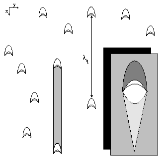
Figure 8: The flux screening length is the mean free path along the wind direction. In other words, it is the mean longitudinal distance between two dunes. Inset: the sand flux is much larger on the back of the dune (dark zone) than on the surrounding ground (gray zone). Downwind the dune, it becomes inhomogeneous and in particular, it is null inside the recirculation bubble (white zone) and low in the triangular shadow zone (light grey). After few dune sizes, the diffusion of grains rehomogenizes the flux.

The distance $\lambda_{q}$ over which the flux changes is thus the distance, along the wind direction, between two dunes. It is the mean free path of one grain traveling in straight line along the wind direction. Let us consider an homogeneous dune field composed of identical dunes of width $w_{\infty}$. The number of dunes per unit surface is $N_{\infty}$. It can be inferred from figure 8 that on average there is one dune in the surface $\lambda_{q}w_{\infty}$ (colored in gray on figure 8). The flux screening length thus depends on the density of dunes as:

$$\lambda_{q}=\frac{1}{N_{\infty}w_{\infty}}.$$ (17)

Note that this length is larger than the average distance $(N_{\infty})^{-1/2}$ between dunes – just like the mean free path in a gas. Since the grains in saltation on the solid ground go much faster than the dune (by more than five orders of magnitude), the flux screening time $\tau_{q}$ can be taken as null:

$$\tau_{q}=0.$$ (18)

II.4 Orders of magnitude

These different time scales can be estimated using the orders of magnitude obtained from field observations in the region of figure 1. The velocity/width relationship has allowed to estimate $aQ\sim 3700~{}m^{2}/year$ and $w_{c}\sim 33~{}m$ in this region. Combined with $\mbox{{C}}_{\mbox{{c}}}^{\mbox{{c}}}$ model results, this gives estimates of the saturation length $L=~{}3.5m$, the minimal horn width $\Delta=4.6~{}m$ and the saturated flux far from any dune $Q\sim 66~{}m^{2}/year$. These values are corroborated by direct measurements of these quantities B41 ; ACD02a .

Let us consider a small dune of width $20~{}m$ and a large dune of width $100~{}m$ belonging to the corridors of dunes shown on figure 1. The distance $\lambda_{r}$ covered by the dune before the equilibrium between the size and the sand flux be reached is respectively $160~{}m$ and $4~{}km$. In all the cases, it is much smaller than the dune field extension (typically $100~{}km$ corresponding to $5000$ small dune widths or $1000$ large dune widths). Obviously, $\lambda_{r}$ is much larger than the turnover length $\lambda_{t}=w$, and it is therefore clear that the turnover scales does not represent the memory of the dune.

The density of dunes can be inferred from figure 1 and is around $0.1~{}{/w^{2}_{\infty}}$ (the average distance between dunes is around $3$ dune sizes). Directly from figure 1 or from formula (17), the flux adaptation length $\lambda_{q}$ is around $10$ dune sizes i.e. $200~{}m$ for the small dune and $1~{}km$ for the large one. Obviously, $\lambda_{q}$ can be very different from place to place. For instance, the left corridor shown on figure 1 is much denser than the third from the left. If the density of small dunes is $1~{}{/w^{2}_{\infty}}$ instead of $0.1~{}{/w^{2}_{\infty}}$, $\lambda_{q}$ becomes equal to the dune size ($20~{}m$).

Using the previous value of $Q$, the dune velocities are $180~{}m/year$ and $37~{}m/year$ for the $20~{}m$ and $100~{}m$ barchans respectively. The corresponding turnover times $\tau_{t}$ are $5.2~{}weeks$ and $2.7~{}years$, while the relaxation time $\tau_{r}$ is as large as $10~{}months$ for the small dunes and $1.1~{}century$ for the large ones. Finally, the flux adaptation time $\tau_{q}$ is equal to the flux screening length $\lambda_{q}$ divided by the grain speed ($\sim 1~{}m/s$). It can thus be estimated to $3~{}minutes$ for $20~{}m$ barchans and $16~{}minutes$ for the $100~{}m$ ones.

The scale separation of the three times is impressive. $\tau_{q}\sim 3~{}minutes\ll\tau_{t}\sim 5.2~{}weeks\ll\tau_{r}\sim 10.4~{}months$ for the small dunes, whereas for the large ones it reads $\tau_{q}\sim 16~{}minutes\ll\tau_{t}\sim 2.7~{}years\ll\tau_{r}\sim 1.1~{}century$. This shows that the annual meteorological fluctuations (wind, humidity) have potentially important effects: the actual memory time is always larger than seasonal time.

Sauermann has estimated a characteristic time for the evolution of the volume of a $100~{}m$ wide dune. He found several decades S01 , which is comparable to the value we found for $\tau_{r}$. On this basis he concluded that “ considering this timescale it is justified to claim that barchans in a dune field are only marginally unstable.” This is a misleading conclusion as the length $\lambda_{r}$ ($4~{}km$ for $w=100~{}m$) should be compared to the corridor size ($\sim 100~{}km$). Moreover, for small dunes as those on the left corridor of figure 1, $\lambda_{r}$ is found to be as small as $160~{}m$ which is of the order of one hundredth of the portion of field displayed on the photograph. The evolution time and length scales could be thought as ‘very large’ - with respect to human scales – but compared to the dune field size, they turn out to be small. Therefore, barchans have in fact the time and space to change their shape and volume along the corridors.

III Flux instability

III.1 Stability of a solitary barchan

We seek to understand the generality of the instabilities revealed by the $\mbox{{C}}_{\mbox{{c}}}^{\mbox{{c}}}$ model. We will first investigate theoretically the stability of a solitary dune in a constant sand flux $q$. We recall that the overall volume of sand received by this dune per unit time is simply proportional to its width: $\phi_{in}=qw$. As found in the $\mbox{{C}}_{\mbox{{c}}}^{\mbox{{c}}}$ model, we suppose that $\phi_{out}=Q(\Delta+\alpha w)$ (figure 9 left). Let us investigate what happens for different values of the input flux $q$.

If $q<\alpha$ (dot-dashed line) the two curves $\phi_{in}(w)$ and $\phi_{out}(w)$ do not cross, which means that no steady solution can be found. Since the input sand volume rate is too low, any dune will shrink and eventually disappear. On the other hand, a fixed point $w_{\infty}$ does exist for $q>\alpha$ (thin solid line). Suppose that this dune is now submitted to a slightly larger (resp. smaller) flux $q$ (dotted lines): it will grow (resp. shrink). However, the corresponding steady states are respectively smaller and larger, so that they cannot be reached dynamically. We now fix the input flux to $q_{\infty}$ and change the dune size $w$, as in figure 5. A dune of width slightly smaller than $w_{\infty}$ under will shrink more and more because it looses sand more than it earns. In a similar way, a dune larger than $w_{\infty}$ will ever grow. In other words, the steady solutions are unstable.

This mechanism explains the flux instability of $\mbox{{C}}_{\mbox{{c}}}^{\mbox{{c}}}$ barchans. This stability analysis is in fact robust and not specific to the linear choice for $\phi_{out}$. Any more complicated function would lead to the same conclusion provided that $\phi_{in}$ crosses $\phi_{out}$ from below. The stability only depends on the behavior of the $\phi$’s in the neighborhood of the steady state.

How could a solitary barchan be stable? It is enough that $\phi_{in}$ crosses $\phi_{out}$ from above. Without loss of generality, we can keep a linear dependence of $\phi_{out}$ on $w$ in the vicinity of the fixed point, but this time with $\Delta<0$ (figure 9 right). In this case, the situation for which the input sand flux $q$ is larger than $\alpha$ (dot-dashed line) leads to an ever growing dune. Steady solutions exist when $q<\alpha$. Because a smaller (resp. larger) sand flux now corresponds to a smaller (resp. larger) dune width, these solutions are, by contrast, stable.

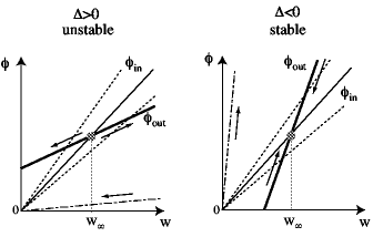
Figure 9: The output volume rate $\phi_{out}=Q(\Delta+\alpha w)$ gives, when compared to the input rate $\phi_{in}=qw$, steady solutions that are unstable if $\Delta>0$, and stable if $\Delta<0$. The main point is to see whether the two lines cross from below or above at the steady point.

In a more quantitative and formal way, the mass balance for a barchan (14) can be rewritten in terms of the dune width only:

$$\dot{w}=\frac{q_{\infty}w-Q(\Delta+\alpha w)}{3bw^{2}}.$$ (19)

Linearizing this equation around the fixed point $w_{\infty}$ we obtain:

$$\tau_{r}\dot{w}=w-w_{\infty}.$$ (20)

The sign of the relaxation time $\tau_{r}$ is that of $\Delta$ – see relation (15). Therefore if $\Delta$ is positive, $w$ will quickly depart from its steady value $w_{\infty}$. In the inverse case $\Delta<0$, any deviation of $w$ will be brought back to $w_{\infty}$.

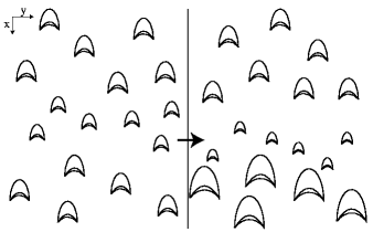
Figure 10: Sketch showing the instability due to the exchange of mass between the dunes: dunes slightly smaller than $w_{\infty}$ loose sand and make their downwind neighbors grow. Note that the dune field is assumed to remain locally homogenous.

In summary, the stability of a solitary barchan depends whether the ratio of the output volume rate to its width $\phi_{out}/w$ increases or decreases with $w$. This quantity is perhaps not easy to measure on the field but we have shown that it is directly related to the ratio of the size of the horn tips to the dune width. If viewed from the face, the horn tips become in proportion smaller as the dune size increases, the barchan is unstable. This is what is predicted by the $\mbox{{C}}_{\mbox{{c}}}^{\mbox{{c}}}$ model, in agreement with the few field observations SRPH00 .

III.2 Stability of a dune field

At this point, the stability analysis leads to the fact that a single solitary barchan is unstable. Could then dunes be stabilized by their interaction via the sand flux? Let us consider a dune field which is locally homogeneous and composed, around the position ($x$,$y$), barchans of width $w$ with a density $N$. We ignore for the moment the fact that dunes can collide. The conservation of the number of dunes then reads

$$\dot{N}=\partial_{t}N+\partial_{x}(\dot{x}N)+\partial_{y}(\dot{y}N)=0.$$ (21)

The eulerian evolution of the dunes width is given by:

$$\dot{w}=\partial_{t}w+\dot{x}\partial_{x}w+\dot{y}\partial_{y}w.$$ (22)

This equation has to be complemented by the equation governing the evolution of the sand flux $q$ between the dunes which results from the variation of the volume of these dunes (and reciprocally):

$$\partial_{x}q=-N\dot{V}.$$ (23)

These three equations can be closed using the previous modeling of $\dot{x}$, $\dot{y}=0$, $\dot{w}$ and $\dot{V}=3bw^{2}\dot{w}$. Any homogeneous field of barchans of width $w_{\infty}$ and density $N_{\infty}$ is a solution, provided that there is a free flux $q_{\infty}=Q(\Delta/w_{\infty}+\alpha)$ between the dunes.

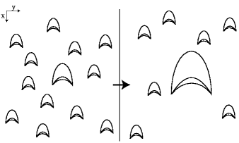
Figure 11: Sketch showing the instability due to the collisions between the dunes. If one dune is slightly larger than the others, it goes slower and will absorb incoming dunes.

We are now interested in the stability of this solution towards locally homogeneous disturbances. Note that such a choice is still consistent with equations that do not take collisions into account. We thus expand $w,q$ and $N$ around their stationary values $w_{\infty},q_{\infty},N_{\infty}$, and introduce the length and time scales $\lambda_{r},\lambda_{q}$ and $\tau_{r}$. We get:

$$\tau_{r}\partial_{t}N + \lambda_{r}\partial_{x}N-\frac{N_{\infty}}{w_{\infty}}\lambda_{r}\partial_{x}w=0,$$ (24)

$$\tau_{r}\partial_{t}w + \lambda_{r}\partial_{x}w=(w-w_{\infty})+\frac{w_{\infty}^{2}}{Q\Delta}(q-q_{\infty}),$$ (26)

$$\lambda_{q}\partial_{x}q=-(q-q_{\infty})-\frac{Q\Delta}{w_{\infty}^{2}}(w-w_{\infty}).$$

Without loss of generality we can write the disturbances under the forms: $q-q_{\infty}=q_{1}e^{\sigma t+ikx}$, $w-w_{\infty}=w_{1}e^{\sigma t+ikx}$ and $N-N_{\infty}=N_{1}e^{\sigma t+ikx}$. Solving the system of linear equations we obtain the expression of the growth rate $\sigma$ as a function of the wavenumber $k$:

$$\tau_{r}\sigma=ik\left(\frac{\lambda_{q}}{1+(k\lambda_{q})^{2}}-\lambda_{r}\right)+\frac{(k\lambda_{q})^{2}}{1+(k\lambda_{q})^{2}}.$$ (27)

The sign of the real part of the growth rate $\sigma$ is that of $\tau_{r}$ and thus of $\Delta$. The stability of the dune field is therefore that of the solitary dune. If $\Delta<0$, which means that all the individual dunes are stable, the field is (for obvious reasons) stable. But in fact, all the individual dunes are unstable ($\Delta>0$), so that a field in which dunes interact via the sand flux is also unstable.

The result of the above formal demonstration, can also be understood via a simple argument illustrated on figure 10. Consider a barchan dune field at equilibrium: for each dune, input and output volume rate are equal. Now, imagine that the input flux of a dune slightly decreases for some reasons. As explained in the previous subsection, if this dune is unstable ($\Delta>0$) it tends to shrink. Consequently its output flux increases, and makes its downwind neighbors grow. Therefore, even a small perturbation of the sand flux can dramatically change the structure of the field downwind.

IV Collisional instability

The free flux is not the only way barchans can influence one another. If sufficiently close, they can interact through the wind, i.e. aerodynamically. This is possible when the dunes get close to each other. In this case, they actually collide. We therefore would like to investigate the behavior of one particular dune in the middle of the field.

Let us consider a homogeneous field of barchans of width $w_{\infty}$, with an additional dune of size $w=(1+\eta)w_{\infty}$. The variation of the volume of this dune is due to the sand flux as well as the collisions of incoming dunes. These collisions are a direct consequence of the fact that smaller dunes travel faster (Eq. 6). The number of collisions per unit time is proportional to the dune density $N_{\infty}$ times the collisional cross section $w+w_{\infty}$ times the relative velocity $aQ~{}(1/w_{\infty}-1/w)$. We assume that the collisions lead to a merging of the two dunes. Then, each collision leads to an increase of the mass of the larger dune by $V_{\infty}=bw_{\infty}^{3}$. We can then write for this particular dune:

$$\dot{V}=qw - Q(\alpha w+\Delta)$$ (28)

$$+ N_{\infty}V_{\infty}(w+w_{\infty})\frac{aQ(w-w_{\infty})}{ww_{\infty}}.$$

Introducing a critical dune density $N_{c}$ as

$$N_{c}=\frac{-\Delta}{2abw_{\infty}^{3}},$$ (29)

the equation governing the evolution of the width of the dune considered reads:

$$\tau_{r}\dot{\eta}=\left(1-\frac{(2+\eta)}{2(1+\eta)}\frac{N_{\infty}}{N_{c}}\right)\frac{\eta}{(1+\eta)^{2}}.$$ (30)

Note that, rigorously speaking, $N_{c}$ is a positive quantity and thus a true density only for $\Delta<0$ (see below). Figure 12 shows $\dot{\eta}$ as a function of the dune size. Expanding linearly around $\eta=0$, we obtain the growth rate $\sigma=\dot{\eta}/\eta$ as:

$$\tau_{r}\sigma=1-\frac{N_{\infty}}{N_{c}}.$$ (31)

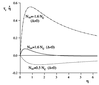
Figure 12: Growth rate $\tau_{r}\dot{\eta}$ of a dune due to collisions, as a function of the rescaled size $\eta$ in three different cases. If the solitary dune is unstable ($\Delta>0$), the field is also unstable towards the collisional instability (dot-dashed line). If the solitary dune is stable ($\Delta<0$), the stability of the field depends on the dune density. At high density (solid line), the field is linearly unstable while at low density (dashed line), it is stable towards any disturbance.

Therefore, if the dunes are individually unstable (case $\Delta>0$, figure 12 a), the dunes are always unstable towards the collisional instability. The barchan field quickly merge into one big barchan dune. If the dune are individually stable ($\Delta<0$), the same instability develops but only when the dune density is larger than the critical dune density $N_{c}$ (figure 12 b). Suppose indeed that one collision occurs in the middle of an homogeneous field, creating a dune of twice its original volume. Since it is larger, this dune slows down and a second collision occurs before the large dune has recovered its equilibrium. If now the dune density is small (figure 12 c), the time before a second collision happens is sufficiently large to allow the large dune to recover its equilibrium volume, and in this case a field of stable dunes is stable towards the collision process.

V Barchans corridors, an open problem

The aim of this conclusion is twofold. We will first give an overview of the different results presented in this paper. Then we will discuss the problem of the size selection and the formation of barchans corridors.

The starting point of the present work is the observation that barchan dunes are organized in fields stretched along the dominant wind direction (figure 1). These barchans corridors are quite homogeneous in size and in spacing. For instance, the barchans field between Tarfaya and Laayoune presents the same five coherent corridors over at least $100~{}km$. This size selection is of course not to be taken in a strict sense: there are large fluctuations from one dune to another, which have also to be explained.

We have shown that the stability of a solitary dune essentially depends on the relationship between the size of the horns and that of the dune. Indeed, the dune receives at its back a sand flux proportional to its size but releases sand only by its horns. If the size of the horns is proportionally smaller for large dunes than for small ones, the steady state of the dune is unstable: it either grows or decay (figure 10). If, on the contrary, the sand leak increases faster than the dune size, it pulls the dune back to equilibrium. Furthermore we have shown that the fact that a dune is fed by the output flux of the dunes upwind does not change the stability analysis. This is essentially because a dune can influence another dune downwind through the flux but there is no feedback mechanism.

We are thus left with a secondary question: how does the horns width evolve with the dune size? The only field measurements from which the horns size can be extracted are the shape measurements of eight dunes by Sauermann et al. SRPH00 . The sum of the width of the two horns is found to be between $12$ and $28~{}m$ for the five small dunes they measured ($2$ and $3~{}m$ high), and between $12$ and $17~{}m$ for the three larger ones (heights between $6$ and $8~{}m$). If we trust the relevance of their selection of dunes, this means that the horn size is almost independent of that of the dune. This is also coherent with their claim that the slip face is proportionally smaller and the horns larger for small dunes than for large ones. In that case, solitary barchans should be individually unstable.

The second indication is provided by the $\mbox{{C}}_{\mbox{{c}}}^{\mbox{{c}}}$ modeling, with which we recover that this steady state is in fact unstable (figures 5 and 7), in fact for the very same reasons as above. The solution can be artificially stabilized by putting at the back of the dune exactly what it looses by its horns but this is only a numerical trick. What determines the size of the horns in the model? The 3D solutions can be thought of coupled 2D solutions ACD02b . Then, the horns start when there is no slip face, i.e. when the length becomes of the order of the minimal size of dunes. This simple argument leads to think that the horns should keep a characteristic size of order of few saturation lengths $L$ whatever the dune size is.

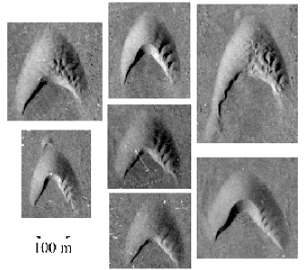
Figure 13: Aerial photographs of several barchan dunes in the same region as the field of figure 1. They all exhibit an instability on the left side, leading to a periodic array of small slip-faces.

We have shown that there is a second robust mechanism of instability. We know from field measurements, numerical models and theoretical analysis that the dune velocity is a decreasing function of its size. The reason is simply that the flux at the crest is almost independent of the dune size and will make a small dune propagate faster than a large one. This is sufficient to predict the coarsening of a dune field: because they go faster, small dunes tend to collide the large ones making them larger and slower…This collision instability should also lead to an ever growing big dune.

The scales over which all instabilities develop are the relaxation time $\tau_{r}$ and length $lambda_{r}$. For the eastern corridor of figure 1, the order of magnitude of the dune width is $100~{}m$ which gives $\tau_{r}\sim 1.1~{}century$ and $\lambda_{r}\sim 4~{}km$. For the western corridors, the dunes are smaller ($w\sim 20~{}m$ and the characteristic scales become $\tau_{r}\sim 10~{}months$ and $\lambda_{r}\sim 160~{}m$. These lengthes are much smaller than the extension of the corridor ($300~{}km$) so that these instabilities have sufficient space to develop.

However, the actual barchan corridors are homogenous and one cannot see any evidence of such instabilities. As a conclusion, the dune size selection and the formation of barchan corridors are still open problems in the present state of the art. There should exist another robust dynamical mechanism leading to an extra-leak of the dunes, to balance the collisional and the flux instabilities. There are already two serious candidates for this mechanism. First, we do not have any information on the collision process. In the $\mbox{{C}}_{\mbox{{c}}}^{\mbox{{c}}}$ model presented here, the collision of two dunes leads to a merging into a larger dune, but in the reality, it could lead to the formation of several dunes. Second, we have only investigated here the case of a permanent wind. We have shown that the dunes characteristic times are larger than one year so that the annual variations of the wind regime could have drastic effects. Figure 13 shows aerial photographs of eight barchan dunes. They all present an instability on their left side, leading to the formation of a periodic array of $1~{}m$ high slip faces. This asymmetry suggests that it is due to a secondary wind (probably a storm) coming from the west (from the left on the figure). This instability could lead to a larger time averaged output flux than expected for a permanent wind. Further work in that direction will perhaps shed light on the formation of nearly homogeneous corridors of barchan dunes.

 

The authors wish to thanks S. Bohn, L. Quartier, B. Kabbachi and Y. Couder for many stimulating discussions.

Appendix: the 3D $\mbox{{C}}_{\mbox{{c}}}^{\mbox{{c}}}$ model

The three starting equations of the model are the conservation of matter, the charge equation and the coupling between the saturated flux and the dune shape $h$:

$$\partial_{t}h+\partial_{x}q = D\,\vec{\nabla}\cdot(q\vec{\nabla}h),$$ (32)

$$\partial_{x}q = \frac{q_{sat}-q}{L},$$ (33)

$$\frac{q_{sat}}{Q} = 1+A\int\!\!\frac{d\chi}{\pi(\chi-x)}\,\partial_{x}h_{e}+B\,\partial_{x}h_{e}.$$ (34)

We recall that the overall flux is the sum of $q$ along the wind direction, plus an extra flux due to reptons along the steepest slope. The two last equations do not contain any $y$ dependence and can thus be solved for each slice in $x$ independently, using a discrete scheme in space ($dx$). The conservation of matter (32) couples the slices through the diffusion term and is solved by a semi-implicit scheme of time step $dt$. To speed up the numerical computation of the saturated flux, we use the discrete Fourier transform ${\cal F}$ of the dune envelope $h_{e}$:

$$q_{sat}=Q\left(1+{\cal F}^{-1}\left\{{\cal F}(h_{e})(A|k|+iBk)\right\}\right).$$ (35)

This envelope is composed of the dune profile $h(x)$ up to the point where the turbulent boundary layer separates:

$$x<x_{b}\,:h_{e}(x)=h(x).$$ (36)

In the absence of any systematic and precise studies on this separation bubble, we assume that the separation occurs when the slope is locally steeper than a critical value $\mu_{b}=0.25$:

$$h(x_{b})-h(x_{b}+dx)>\mu_{b}dx.$$ (37)

When the dune presents a slip face, the boundary layer thus separates at the crest. The separation streamline is modeled as a third order polynomial:

$$x_{b}<x<x_{r}\,:h_{e}(x)=a+bx+cx^{2}+dx^{3}.$$ (38)

The four coefficients are determined by smooth matching conditions:

$$h_{e}(x_{b})=h(x_{b}), h_{e}(x_{b}-dx)=h(x_{b}-dx),$$ (39)

$$h_{e}(x_{r})=h(x_{r}), h_{e}(x_{r}+dx)=h(x_{r}+dx),$$ (40)

and the reattachment point $x_{r}$ is the first mesh point for which the slope is nowhere steeper than $\mu_{b}$. There is no grain motion inside the recirculation bubble, so that the charge equation should be modified to $\partial_{x}q=-q$ for $x_{b}<x<x_{r}$. Similarly, on the solid ground ($h=0$) no erosion takes place, so that $\partial_{x}q=0$.

The last important mechanism is the relaxation of slopes steeper than $\mu_{d}$ by avalanching. Rather than a complete and precise description of avalanches of grains, we treat them as an extra flux along the steepest slope:

$$\partial_{t}h+\partial_{x}q=\vec{\nabla}\cdot[(Dq+E\delta\mu)\vec{\nabla}h],$$ (41)

where $\delta\mu$ is nul when the slope is lower than $\mu_{d}$ and equal to $\delta\mu=|\vec{\nabla}h|^{2}-\mu_{d}^{2}$ otherwise. For a sufficiently large coefficient $E$, the result of this trick is to relax the slope to $\mu_{d}$, independently of $E$. Note that, as the diffusion of reptons, these avalanches couple the different 2D slices. The value of the parameters have been chosen to reproduce the morphological aspect ratios and are given in the following table:

$A=4.7$	curvature effect
$B=5.0$	slope effect
$D=0.1$	Lateral diffusion
$\mu_{b}=0.25$	separation slope
$E=50$	avalanches
$\mu_{d}=0.5$	avalanche slope
$dx=0.25-1.0$	grid step
$dt=0.001-0.1$	time step
$M=64-512$	box size

The results presented in this paper have been obtained for different discretization time and space steps, different box sizes and different total times. This explains the slight dispersion of the measurements.

References

- (1) R.A. Bagnold, The physics of blown sand and desert dunes, Chapman and Hall, London (1941).
- (2) P.R. Owen, Saltation of uniform grains in air, J. Fluid. Mech. 20, 225-242 (1964).
- (3) A.D. Howard, Effect of slope on the threshold of motion and its application to orientation of wind ripples, Bulletin Geological Society of America 88, 853-856 (1977).
- (4) M. Sørensen, Estimation of some aeolian saltation transport parameters from transport rate profiles, in International workshop on the physics of blown sand, Barndorff-Nielsen, Moller, Rasmussen and Willets eds. University of Aarhus, 141-190 (1985).
- (5) J.L. Jensen and M. Sorensen, Estimation of some aeolian saltation transport parameters: a re-analysis of Williams data, Sedimentology 33, 547-558 (1986).
- (6) R.S. Anderson and P.K. Haff, Simulation of aeolian saltation, Science 241, 820-823 (1988).
- (7) R.S. Anderson and P.K. Haff, Wind modification and bed response during saltation of sand in air, Acta Mechanica [Suppl]1, 21-51 (1991).
- (8) R.S. Anderson, M. Sørensen and B.B. Willetts, A review of recent progress in our understanding of aeolian sediment transport, Acta Mechanica [Suppl]1, 1-19 (1991).
- (9) M. Sørensen, An analytic model of wind-blown sand transport, Acta Mechanica [Suppl]1, 67-81 (1991).
- (10) B.B. Willetts, J.K. McEwan and M.A. Rice, Initiation of motion of quartz sand grains, Acta Mechanica [Suppl] 1, 123-134 (1991).
- (11) K.R. Rasmussen, H.E. Mikkelsen, Wind tunnel observations of aeolian transport rates, Acta Mechanica [Suppl]1, 135-144 (1991).
- (12) P. Nalpanis, J.C.R. Hunt and C.F. Barrett, Saltating particles over flat beds, J. Fluid Mech. 251, 661-685 (1993).
- (13) J.D. Iversen and K.R. Rasmussen, The effect of surface slope on saltation threshold, Sedimentology 41, 721-728 (1994).
- (14) K.R. Rasmussen, J.D. Iversen and P. Rautaheimo, Saltation and wind flow interaction in a variable slope wind tunnel, Geomorphology 17, 19-28 (1996).
- (15) F. Rioual, A. Valance and D. Bideau, Experimental study of the collision process of a grain on a two-dimensional granular bed, Phys. Rev. E 62, 2450-2459 (2000).
- (16) G. Sauermann, K. Kroy and H.J. Herrmann, A continuum saltation model for sand dunes, Phys. Rev. E 64, 031305 (2001).
- (17) B. Andreotti, A two species model of aeolian sand tranport, submitted to J. Fluid Mech. (2003).
- (18) H.J.L. Beadnell, The sand-dunes of the Libyan desert, Geographical Journal 35, 379-395 (1910).
- (19) H.J. Finkel, The barchans of southern Peru, Journal of Geology 67, 614-647 (1959).
- (20) A. Coursin, Bulletin de l’IFAN 3, 989-1022 (1964).
- (21) J.T. Long and R.P. Sharp, Barchan dune movement in imperial valley, California, Geological Society of America, 75, 149-156 (1964).
- (22) S.L. Hastenrath, The barchans of the Arequipa Region, Southern Peru, Zeitschrift für Geomorphologie 11, 300-331 (1967).
- (23) R.M. Norris, Barchan dune of imperial valley, California, J. Geol. 74, 292-306, (1966).
- (24) S.L. Hastenrath, The barchans of Southern Peru revisited, Zeitschrift für Geomorphologie 31-2, 167-178 (1987).
- (25) M.C. Slattery, Barchan migration on the Kuiseb river delta, Namibia, South African Geographical Journal 72, 5-10 (1990).
- (26) P.A. Hesp and K. Hastings, Width, height and slope relationships and aerodynamic maintenance of barchans, Geomorphology 22, 193-204, (1998).
- (27) G. Sauermann, P. Rognon, A. Poliakov and H.J. Herrmann, The shape of barchan dunes of southern Morocco, Geomorphology 36, 47-62 (2000).
- (28) B. Andreotti, P. Claudin and S. Douady, Selection of dune shapes and velocities. Part 2: A two-dimensional modelling, Eur. Phys. J. B 28, 341-352 (2002).
- (29) P. Hersen, S. Douady and B. Andreotti, Relevant lengthscale of barchan dunes, Phys. Rev. Lett. 89, 264301, (2002).
- (30) K.R. Mulligan, Velocity profiles measured on the windward slope of a transverse dune, Earth surface processes and Landforms 13, 573-582 (1988).
- (31) O. Zeman and N-O. Jensen, Modification of turbulence characteristics in flow over hills, Quart. J. R. Met. Soc. 113, 55-80(1987).
- (32) P.S. Jackson and J.C.R. Hunt, Turbulent wind flow over a low hill, Quart. J. R. Met. Soc. 101, 929-955 (1975).
- (33) A.D. Howard, J.B. Morton, M. Gad el Hak and D.B. Pierce, Sand transport model of barchan dune equilibrium, Sedimentology 25, 307-338 (1978).
- (34) N-O. Jensen and O. Zeman, in International workshop on the physics of blown sand, Barndorff-Nielsen, Moller, Rasmussen and Willets eds. University of Aarhus, 351-368 (1985).
- (35) F.K. Wippermann and G. Gross, The wind-induced shaping and migration of an isolated dune: numerical experiment, Boundary-Layer Meteorology 36, 319-334 (1986).
- (36) J.C.R. Hunt, S. Leibovitch and K.J. Richards, Turbulent shear flows over low hills, Quart. J. R. Met. Soc. 114, 1435-1470 (1988).
- (37) W.S. Weng, J.C.R. Hunt, D.J. Carruthers, A. Warren, G.F.S. Wiggs, I. Livingstone and I. Castro, Air flow and sand transport over sand-dunes, Acta Mechanica [Suppl] 2, 1-22 (1991).
- (38) B.T. Werner, Aeolian dunes: computer simulations and attractor interpretation, Geology 23, 1107-1110 (1995).
- (39) J.H. van Boxel, S.M. Arens, P.M. van Dijk, Aeolian processes across transverse dunes. I: Modelling the air flow, Earth Surface Processes and Landforms 24, 255-270 (1999).
- (40) K. Kroy, G. Sauermann and H.J. Herrmann, A minimal model for sand dunes, Phys. Rev. Lett. 88, 054301 (2002)
- (41) G. Sauermann, PhD Thesis, Stuttgart University, edited by Logos Verlag (Berlin) (2001).
- (42) B. Andreotti, P. Claudin and S. Douady, Selection of dune shapes and velocities. Part 1: Dynamics of sand, wind and barchans, Eur. Phys. J. B 28, 321-339 (2002).
- (43) K. Lettau and H.H. Lettau, Bulk transport of sand by the barchans of La Pampa La Hoja in southern Peru, Zeitschrift für Geomorphologie 13, 182-195 (1969).
- (44) A.R. Lima, G. Sauermann, H.J. Herrmann, K. Kroy, Modelling a dune field, Physica A 310, 487-500 (2002).
- (45) P. Hersen, On the crescentic shape of barchan dune, submitted to EPJ. B. (2003).