Dissipative flow and vortex shedding in the Painlevé boundary layer of a Bose Einstein condensate

Abstract

Raman et al.R have found experimental evidence for a critical velocity under which there is no dissipation when a detuned laser beam is moved in a Bose-Einstein condensate. We analyze the origin of this critical velocity in the low density region close to the boundary layer of the cloud. In the frame of the laser beam, we do a blow up on this low density region which can be described by a Painlevé equation and write the approximate equation satisfied by the wave function in this region. We find that there is always a drag around the laser beam. Though the beam passes through the surface of the cloud and the sound velocity is small in the Painlevé boundary layer, the shedding of vortices starts only when a threshold velocity is reached. This critical velocity is lower than the critical velocity computed for the corresponding 2D problem at the center of the cloud. At low velocity, there is a stationary solution without vortex and the drag is small. At the onset of vortex shedding, that is above the critical velocity, there is a drastic increase in drag.

Dilute Bose-Einstein condensates have recently been achieved in confined alkali-metal gases and the study of vortices therein is one of the key issues. Raman et al. R ; RO , Onofrio et al. O have studied dissipation in a Bose Einstein condensate by moving a blue detuned laser beam through the condensate at different velocities. They found experimentally a critical velocity for the onset of dissipation. This critical velocity has been related to the one found by Frisch et al. FPR for the problem of a 2D superfluid flow around an obstacle in the framework of Nonlinear Schrodinger Equation (NLS): below a critical velocity, the flow is stationary and dissipationless, while beyond this critical velocity, the flow around the disc becomes time dependent and vortices are emitted. Numerical simulations have been done for this type of problem in 2D HB and 3D JMA ; W . In particular, the direct 3D simulation of W shows the plot of the drag against the velocity. A critical velocity can be numerically computed when the drag becomes nonzero, but no precise mechanism of vortex nucleation is described by the authors. This critical velocity has been analyzed theoretically for a homogeneous 2D system SZ and an inhomogeneous 2D system C ; FS .

In this paper, we want to take into account the 3D geometry of the experiment of R ; O ; RO . Our aim is to understand the mechanism of vortex nucleation in the boundary region. Indeed the analysis of FPR allows to understand what is happening in the interior of the cloud, where the kinetic energy is negligible in front of the interaction energy. In the region where the laser beam crosses the boundary of the cloud, the sound velocity gets small, since the amplitude of the wave function becomes small. There, the kinetic energy term can no longer be neglected in front of the trapping and interaction terms. We blow up this region in such a way that the trapping potential varies linearly with the distance to the boundary and far away from the laser beam, the wave function is then given by a Painlevé equation. We analyze the behavior of the wave function in the frame of the laser beam. The real experiments are quite complex, and in particular here we do not take into account the oscillations and acceleration of the beam but we believe that our analysis allows to understand the mechanism of increase of drag. One of our main results is that there is always a drag around the laser beam and this drag grows continuously. At low velocity, the drag is not a consequence of the shedding of vortices, and finally of a time dependent density and velocity field. The origin of this drag is in the radiation condition for the wavefield: the motion changes continuously the structure of the solution seen in the frame of reference of the ”fluid” at infinity. We study the transition toward a time dependent regime of vortex shedding, which happens at a critical velocity. The critical velocity that we find is lower than the 2D critical velocity at the center of the cloud coming from the computation of FPR . Vortices are nucleated close to the boundary of the cloud and the tubes grow and detach to form rings that move downstream. When tubes are emitted, significantly large drag values are observed. The drag increases smoothly as the velocity increases.

The dynamics can be modeled using the Gross Pitaevskii equation at zero temperature with an external trapping potential $V_{tr}=m/2(\omega_{x}^{2}x^{2}+\omega_{y}^{2}y^{2}+\omega_{z}^{2}z^{2})$.

$$i\hbar\partial_{t}\Psi=-{{\hbar^{2}}\over{2m}}\Delta\Psi+(V_{tr}+Ng|\Psi|^{2})\Psi.$$

If an object is moved inside the condensate, $V_{tr}$ has to be replaced by $V_{tr}+V_{ob}$, where $V_{ob}$ depends on $x-vt$. Based on the experimental data of R ; O , we take $a=mg/4\pi\hbar^{2}=2.94\ nm$, $N=1.2.10^{7}$, $\omega_{y}=\omega_{z}=377s^{-1}$, and $\omega_{x}=\lambda\omega_{z}$, with $\lambda=0.3$. We also define the characteristic length $d=(\hbar/m\omega_{z})^{1/2}=2.71\ \mu m$ and a small nondimensionnalized parameter $\varepsilon$ given by

$$\varepsilon=({{d}\over{8\pi Na}})^{2/5}.$$

We find that $\varepsilon=6.21\ 10^{-3}$ which may be viewed as small parameter and allow rescaling the equation near the edge of the condensate. Re-scaling the distances by $R=d/\sqrt{\varepsilon}=34.4\ \mu m$, the time by $1/(\varepsilon\omega_{z})$, we have $\psi({\bf r},t)=R^{3/2}\phi({\bf\tilde{r}},{\tilde{t}})$ where ${\bf\tilde{r}}=R{\bf r}$. In these new units, the radii of the condensate are $R_{y}=R_{z}=0.65$ and $R_{x}=2.18$. The laser beam is modeled by an obstacle which is a cylinder ${\cal C}$ of axis $z$ and radius $l=0.19$ on which $\psi=0$. We will work in the frame where the obstacle is stationary. Outside the obstacle, the equation can be rewritten as

$$-2i\partial_{t}\psi=\Delta\psi+{1\over\varepsilon^{2}}(\rho_{TF}-|\psi|^{2})\psi,$$

where $\rho_{TF}=\rho_{0}-(\lambda^{2}x^{2}+y^{2}+z^{2})$ is the Thomas Fermi limit density and $\rho_{0}=0.42$ is the rescaled chemical potential. Note that $|\psi|^{2}$ is close to its Thomas Fermi value $\rho_{TF}$ except near the obstacle and near the boundary of the cloud. This boundary layer has a thickness of order $\varepsilon^{2/3}$ so that we rescale the domain with $\psi({\tilde{x}},{\tilde{y}},{\tilde{z}})=\varepsilon^{1/3}u(x,y,z)$, where $x={\tilde{x}}/\varepsilon^{2/3}$, $y={\tilde{y}}/\varepsilon^{2/3}$ and $z=(\sqrt{\rho_{0}}-{\tilde{z}})/\varepsilon^{2/3}$, $v={\tilde{v}}\varepsilon^{2/3}$. By blowing up the boundary of the cloud near $z=0$, and truncating at $z=L$, the rescaled layer thickness, we see that the modulus of the stationary solution in the boundary layer for $|x|$ and $|y|$ large, that is far away from the obstacle, is given by the solution of the first Painlevé equation FF ; DPS .

$$p^{\prime\prime}+(2z\sqrt{\rho_{0}}-p^{2})p=0,\ p(0)=0,\ p(L)=\sqrt{2\sqrt{\rho_{0}}L}.$$ (1)

We choose the size of the boundary layer $L$ so that $\varepsilon^{2/3}L=3\sqrt{\rho_{0}}/10$. This is based on the consideration that, on the one hand, $\varepsilon^{2/3}L$ should be suitably small so that $2z\sqrt{\rho_{0}}$ is a good approximation for $\rho_{TF}=\rho_{0}-{\tilde{z}}^{2}$ in the boundary layer and on the other hand the critical velocity at $z=L$ is not too different from the critical velocity at the center of the cloud. The obstacle is now a cylinder of radius $a=l/\varepsilon^{2/3}=5.6$.

The obstacle moves at the rescaled velocity $v=v_{exp}/(\varepsilon^{1/3}\omega_{z}R)$, and in the frame of the obstacle, the equation becomes

$$-2i\partial_{t}u=\Delta u-2iv\partial_{x}u+(2z\sqrt{\rho_{0}}-|u|^{2})u.$$ (2)

We want to understand the behaviour of solutions depending on $v$. If we restrict (2) to $z=L$, we can perform a similar analysis to FPR and get the value of the critical velocity for the onset of vortex shedding and find $v_{c}^{2}=2\sqrt{\rho_{0}}L/11=2c_{s}^{2}/11$, where $c_{s}$ is the sound velocity. Of course, we cannot apply this analysis in the low density region, since there the sound velocity gets close to 0. Another mechanism has to be understood. The rescaled drag around the obstacle is

$$drag=\frac{1}{2}\int_{\cal C}(u_{x}\bar{u}_{n}-\bar{u}_{x}u_{n})\;dl\ dz.$$ (3)

We first analyze the stationary solution of (2) in the very low density region, where the system is very dilute and one can neglect the nonlinear term. In fact, a precise condition is that $p^{2}$ is less than $v^{2}$, which gives a truncation point $z_{c}$ at which $p^{2}(z_{c})=v^{2}$. It is rather straightforward in classical scattering theory to compute the perturbed wavefield and finally the drag on the obstacle (a related problem, the scattering of sound by a cylinder, is treated in M ). In the low density region, it is reasonable to look for $u$ with the following ansatz

$$u(x,y,z)=p(z)\psi(x,y)e^{ivx}.$$ (4)

We can first approximate $p(z)$ in this region by an Airy function given by the solution of $p^{\prime\prime}+2zp\sqrt{\rho_{0}}=0$, that is, by defining $\overline{z}^{3}=1/(2\sqrt{\rho_{0}})$, we have

$$p(z)\approx\sqrt{2}Ai({{-z}\over{\overline{z}}})\approx{1\over{\sqrt{2\pi}}}({{{-\overline{z}}\over{z}}})^{1\over 4}exp(-{2\over 3}({{-z}\over{\overline{z}}})^{3\over 2}).$$ (5)

Then, outside the obstacle, $\psi$ is a solution of the 2D Helmholtz equation

$$\Delta\psi+v^{2}\psi=0$$ (6)

with $\psi=0$ for $r=a$, the obstacle boundary, and $\psi\approx e^{ivx}$ at infinity. This solution can be computed M in terms of Bessel functions $J_{k}$ and $N_{k}$. One finds that, at leading order for $v$ small, the 2D drag of $\psi$ is proportional to

$$v^{2}J_{0}^{2}(v)J_{1}(v)N_{2}(v)/N_{0}^{2}(v)\sim v/\log^{2}v.$$ (7)

The total drag has to be multiplied by the integral of $p^{2}$ along the $z$ axis to the truncation point $z_{c}$ defined by $p^{2}(z_{c})=v^{2}$. Direct calculation gives

$${v\over{\log^{2}v}}\int_{-\infty}^{z_{c}}p^{2}\ dz\approx C{{v^{3}}\over{\log^{8/3}v}}.$$ (8)

In conclusion, the total scattering drag tends to zero at low speed. It is plotted in Figure 1 (solid line).

To understand how the solutions of (2) behave, we numerically integrate the equation in a computational domain of dimension $60\times 60\times L$ with periodic boundary conditions in $x$ and $y$ and taking $u=0$ on the boundary of the obstacle and away from the condensate ($z=0$). At the truncated surface $z=L$ inside the condensate, we use the condition $({\partial}/{\partial z})(u/p)=0$, where $p$ is the solution to the Painlevé equation (1) described before. The numerical solution is computed based on a continuous piecewise quadratic finite element approximation in space and the Runge-Kutta fourth-order in time integration scheme. Using $p$ as initial condition, we first compute the solution of (2) for some time by adding a damping coefficient, that is, we replace $iu_{t}$ in (2) by $iu_{t}(1+i\gamma)$. For small velocity, this effectively drives the numerical solution of (2) close to a stationary solution. Then, we continue the integration with a much reduced damping coefficient $\gamma=0.02$ or with no damping $\gamma=0$.

In what follows, we will divide the velocity by the sound velocity at center $c_{s}=\sqrt{2\rho_{0}}/\varepsilon^{1/3}$. In Figure 1, we plot the drag vs. the velocity divided by $c_{s}$. For a given velocity value, the drag is the value obtained through time averaging of (3). We have verified that with different small values of $\gamma$, the drag calculation remains essentially the same.

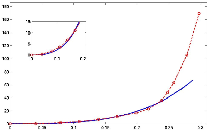
Figure 1: Drag vs. $v/c_{s}$: $--$ for (8), $-o-$ for numerical solution of (2); insert: zoomed in for small $v$.

For $v$ small, we find that the solution is almost stationary. Surface oscillations are present near $z=0$, and the drag is small, but not zero. See Figure 2 for plots of the solution. The drag computed in this regime fits very well to the cubic growth given by (8).

When $v$ is increased, at a critical velocity $v_{c}/c_{s}\approx 0.2$, the surface oscillations develop into small handles that move up and down the obstacle without detaching; see Figure 3.

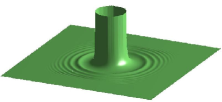
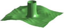
Figure 2: Isosurface snapshot of $|u|$: surface waves for $v=0.08$ and $v=0.2$.

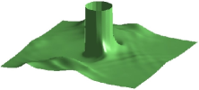
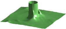
Figure 3: Isosurface snapshots of $|u|$ at different times for $v=0.24$: formation of vortex handles.

There is no stationary solution, but no vortex shedding either: the small handles move up the obstacle to a critical $z$ value and down. This instability may be related to the one discussed by Anglin A1 : in our scaling, the critical velocity found in A1 is 0.2. At this stage, the solutions do not produce large drag nor vortex shedding.

It is only for larger velocities ($v/c_{s}>0.25$) that the handles move up to the top, detach from the obstacle and produce significant drag. This is a wholly nonlinear phenomenon and most likely cannot be described by a linear analysis.

Let us describe the solutions for $v/c_{s}>0.25$ illustrated in Figure 4.

 

 

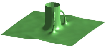
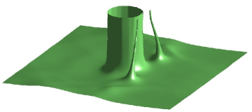
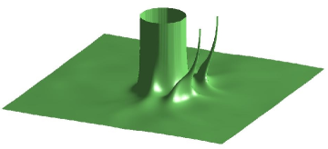
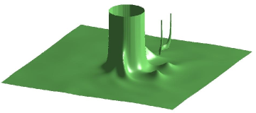
Figure 4: A sequence of isosurface snapshots of $|u|$ for $v=0.28$: a) formation of vortex handles, b) detachment from obstacle, c) bending of vortex tubes and d) formation of vortex half rings.

The vortex handles seem to first nucleate near $z=0$ and are top connected to the obstacle. As time increases, the bottom ends move away from the obstacle in a slightly down stream direction while the top end moves up along the obstacle (Figure 4a). When the top ends of the vortices become close to $z=L$, the bottom ends reverse their trend of moving away from obstacle. Instead, they move back to the bottom of the obstacle, as if the handles prefer certain curvature (Figure 4b). Eventually, the top ends of the handle move away from the obstacle and produce a pair of vortex tubes with their bottom ends at the bottom of the obstacle (Figure 4c). The handles merge into a half vortex ring, this half ring moves both upward and downstream (Figure 4d). Near $z=0$, the solution can be approximated by the solution (4) and this solution does not have vortices, so the instability creates the vortex but the vortex moves away. Vortex detachment happens only at sufficiently high density, in the region where the nonlinear term in the equation dominates. The direction of the vortex displacement is due to the velocity of the flow and the self interaction of the vortex on itself, which gives a movement along its normal vector. Meanwhile, while the vortex ring starts to detach from the obstacle, another pair of vortex handles is forming near the obstacle. The above process repeats itself. Note that we have truncated the domain close to the boundary of the cloud, so that the half ring we compute would correspond to a closed ring in the experiments.

We have to point out that the critical velocity we have found for the onset of vortex shedding is lower than the critical velocity for the 2D problem at $z=L$. In this case $v_{2D}/c_{s}=0.35$. So the inhomogeneity in the condensate lowers the critical velocity from the 2D value. One can check that for different $L$, the critical velocity does not change. This is verified by our numerical computation where we have used two boxes with one about 50% higher in $z$ than the other, and there is little change in the drag plots, nor there is any significant difference in the dynamic behavior of the solutions.

In the experiments R ; RO ; O , the drag is plotted vs velocity and a critical velocity can be defined when a sharp slope is observed in the drag plot. The critical velocity in R is very similar to ours, though slightly smaller. This is certainly due to the finite extent of the condensate in the $x$, $y$ direction. Indeed, our simulations have not taken into account that the cloud is narrower in the $y$ direction than along the $x$. We can check that for the 2D problem, this geometry lowers the velocity. On the other hand, our computations indicate that the inhomogeneity in the $z$ direction and the soft boundary of the laser beam are well accounted for by our problem.

Summary. We have studied the onset of dissipation in the Painlevé boundary layer of a BEC when a detuned laser beam is moved in the condensate. We do a change of frame and blow up the low density region near the boundary of the cloud to write the equation for the wave function in this region: $z=0$ is now the boundary of the cloud and $z$ large is the center. For small velocity, there is a drag around the obstacle due to radiation, but no vortex is generated: it is a stationary flow, which is supersonic near $z=0$, but subsonic for $z$ larger. On the other hand, when the critical velocity is reached, the instability propagates towards the top, a vortex handle is nucleated and detaches from the obstacle to form vortex rings that move away. Our aim was to understand the origin of vortex shedding. The critical velocity is lower than for the 2D problem. There is a drag for all velocity, it increases smoothly with the velocity, and there a significant increase at the onset of vortex shedding.

- (1) C. Raman, M. Köhl, R. Onofrio, D. S. Durfee, C. E. Kuklewicz, Z. Hadzibabic, and W. Ketterle, Phys. Rev. Lett. 83, 2502-2505 (1999).
- (2) R. Onofrio, C. Raman, J. M. Vogels, J. R. Abo-Shaeer, A. P. Chikkatur, and W. Ketterle Phys. Rev. Lett. 85, 2228-2231 (2000).
- (3) C. Raman, R. Onofrio, J. M. Vogels, J. R. Abo-Shaeer and W. Ketterle, J. Low Temp Phys. 122, 99-116, (2001).
- (4) T. Frisch, Y. Pomeau, and S. Rica, Phys. Rev. Lett. 69, 1644 (1992).
- (5) C.Huepe and M.E.Brachet, Physica D 144, 20-36 (2000).
- (6) B. Jackson, J. F. McCann, and C. S. Adams, Phys. Rev. A 61, 051603 (2000).
- (7) T.Winiecki, B Jackson, J F McCann and C S Adams J. Phys. B: At. Mol. Opt. Phys. 33 No 19 (2000) 4069-4078.
- (8) J. S. Stie berger and W. Zwerger Phys. Rev. A 62, 061601 (2000).
- (9) M. Crescimanno, C. G. Koay, R. Peterson, and R. Walsworth Phys. Rev. A 62, 063612 (2000).
- (10) P. O. Fedichev and G. V. Shlyapnikov Phys. Rev. A 63, 045601 (2001).
- (11) F.Dalfovo, L.Pitaevskii and S.Stringari, Phys. Rev. A 54, 4213 (1996).
- (12) A.L.Fetter and D.L.Feder, Phys. Rev. A, 58, 3185 (1998).
- (13) P. Morse and K. Ingard, Theoretical Acoustics, McGraw-Hill, (1968).
- (14) J. R. Anglin, Phys. Rev. Lett. 87, 240401 (2001).