Dynamics of Dissipative Quantum Hall Edges

Abstract

We examine the influence of the edge electronic density profile and of dissipation on edge magnetoplasmons in the quantum Hall regime, in a semiclassical calculation. The equilibrium electron density on the edge, obtained using a Thomas-Fermi approach, has incompressible stripes produced by energy gaps responsible for the quantum Hall effect. We find that these stripes have an unobservably small effect on the edge magnetoplasmons. But dissipation, included phenomenologically in the local conductivity, proves to produce significant oscillations in the strength and speed of edge magnetoplasmons in the quantum Hall regime.

I Introduction

We investigate electron dynamics on the edges of a two-dimensional electron system in the quantum Hallqhe regime. Our aim is to examine the influence of the edge electronic density profile and of dissipation on the low-energy dynamics. Dealing with the combined effects of electron interactions, disorder, and density inhomogeneities is very complicated. Consequently we adopt a simple semiclassical edge magnetoplasmon model, appropriate for smooth edges, with an eye towards explaining the kinds of phenomena that can be expected. This work helps explain some recent dynamical measurements, and may help develop such measurements into a quantitative tool to examine the structure and properties of quantum Hall edges.

This work was motivated by recent time-of-flight experiments by Ernst et al.e1 ; e2 ; e3 on quantum Hall bars. These consist of rectangular two-dimensional (2D) electron systems with strong transverse magnetic fields $B$. In these experiments a voltage pulse sent down a thin ($\sim 1\,\mu$m) voltage probe triggers a density pulse. This pulse moves along the edge and is then detected as a voltage signal at a second probe. The density pulse’s transit time was found to generally increase with magnetic field (a behavior expected classically), but superimposed on this trend were sudden changes associated with the quantum Hall effecte2 ; e3 . The strength of the detected signal showed corresponding variations. A similar technique was used earlier by Ashoori et al. to look for counter-propagating modes on a single mesaashoori ; mjz .

The appropriate framework for studying electronic properties on the edges of Hall bars depends on the ratio of two length scales. These are the edge width $a$ (the distance over which the electron density falls from its bulk value to zero) and the magnetic length $\ell=\sqrt{\hbar c/eB}$ (of order 10 nm for typical magnetic fields). The limiting cases are of sharp edges ($a\sim\ell$) and smooth edges ($a\gg\ell$). Sharp edges can can be obtained by cleavingchang . The electronic properties of sharp edges are largely quantum mechanical in nature, and determined by the state of the bulk. For example, at filling factors $\nu$ ($=2\pi\ell^{2}$ times the bulk two-dimensional density) at which the fractional quantum Hall effect (FQHE) is exhibited, the edge dynamics may be describable in terms of chiral one-dimensional Luttinger liquidswen ; stone ; kane ; pal ; shytov . This possibility has received some experimental support (with a few surprising twists) in measurements of tunneling onto edgeschang ; milliken ; grayson ; conti ; zul ; lee ; levitov ; grayson2 .

In this paper we deal only with the opposite limit of smooth edges, $a\gg\ell$. This is typical in samples which are not cleaved. In the absence of cleaving, the edge structure is determined by the electrostatics of the 2D electron system, donors, and gates. These produce edges with a typical width $a$ of order $1\,\mu$m. This is much greater than the magnetic length $\ell$, so electrostatically-defined edges are smooth. Since the electrostatics dominates, the electron density on the edge is close to the classical solution: a compressible electron gas with a density falling smoothly from its bulk value to zero over a distance $a$. Quantum mechanical energy gaps arising in the quantum Hall regime modify this picture, producing incompressible stripes along the edge at certain filling factorsbeenakker ; chk . Under these circumstances the low-energy edge dynamics is determined largely by the compressible portion of the edge electron density. Then a reasonable framework for beginning a study of the edge dynamics is the semiclassical acoustic edge magnetoplasmonVM ; AG . This is the direction we follow.

In the next section we will summarize existing work which leads to the edge magnetoplasmon. The new results of this paper are then contained in Sections III and IV. In Section III we examine the effect of incompressible stripes on the edge magnetoplasmon. The variation of stripe position and width with magnetic field modifies the edge magnetoplasmon’s velocity, but the effect appears too small to be observable. In Section IV we examine how disorder-induced dissipation both damps and slows the edge modes. In the quantum Hall regime dissipation varies with magnetic field, and so the edge magnetoplasmon’s strength and speed should change simultaneously. We find that this effect is observably large.

II Edge Magnetoplasmons

Edge magnetoplasmons are classical or semiclassical electronic density fluctuations on the edge of a 2D electron system, in the presence of a magnetic field. They are acoustic modes, with frequencies much less than the classical cyclotron frequency $\omega_{c}=eB/mc$. Edge magnetoplasmons have been studied thoroughly in two cases. Volkhov and Mikhailov used a Wiener-Hopf technique to investigate their properties for half spaces (the extreme sharp-edge limit, $a\rightarrow 0$), in the presence of dissipationVM . Later Aleiner and Glazman studied smooth edges in the absence of dissipation, in strong magnetic fieldsAG . They found that the smooth edge can support many modes, with differing numbers of nodes; the fastest, nodeless mode corresponded to the Volkhov-Mikhailov edge magnetoplasmon. In this paper we extend these studies to investigate the roles of differing edge density structures and dissipation in the case of smooth edges. We begin with a summary of the basics of edge magnetoplasmons, following Aleiner and GlazmanAG .

Consider a Hall bar, a 2D electron system in the $xy$ plane subject to a perpendicular magnetic field $\mathbf{B}$ (Fig. 1). To study a single edge we can take the system to be infinite along the edge (coordinate $y$) and semi-infinite in the transverse direction (coordinate $x$). In equilibrium this system is translationally invariant along the edge, and so the equilibrium 2D electronic density $n_{0}(x)$ depends only on the transverse coordinate $x$. We can distinguish bulk and edge regions. In the bulk $n_{0}(x)$ takes a constant bulk value $n_{b}$, and on the edge $n_{0}(x)$ falls from $n_{b}$ to zero. We take the bulk and edge regions to be, respectively, $-\infty<x<0$ and $0<x<a$.

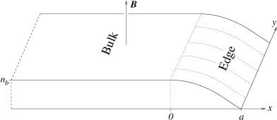
Figure 1: Schematic equilibrium electronic density $n_{0}(x)$ near the edge of a Hall bar. The system is taken to be semi-infinite in the transverse ($x$) direction and infinite in the longitudinal ($y$) direction. In the bulk ($-\infty<x<0$) the density takes the constant value $n_{b}$. On the edge $(0\leq x\leq a$) the density falls from the bulk value to zero.

We also allow the presence of a top gate (a grounded piece of metal parallel to the 2D electron system, a distance $d$ away). The only mobile charges in the system are the electrons in the 2D plane and in the gate (the latter included as image charges). Classically the equilibrium density $n_{0}(x)$ corresponds to a vanishing in-plane electric field. If the electronic density takes a nonequilibrium value $n({\mathbf{r}})=n_{0}(x)+\delta n({\mathbf{r}})$, then the net electric field in the 2D plane, including image charges, becomes

$$\mathbf{E}(\mathbf{r}) = -\nabla\Phi(\mathbf{r}),$$

$$\Phi(\mathbf{r}) = -\frac{e}{\varepsilon}\int d^{2}r^{\prime}\,\delta n({\mathbf{r}^{\prime}})\left(\frac{1}{|\mathbf{r}-\mathbf{r}^{\prime}|}-\frac{1}{[{|\mathbf{r}-\mathbf{r}^{\prime}|^{2}}+(2d)^{2}]^{\frac{1}{2}}}\right).$$ (1)

Here $-e$ is the electronic charge, and $\varepsilon$ is the dielectric constant of the material within which the 2D electron system lies (12.4 for GaAs). This electric field expression is also satisfactory for time-dependent densities $\delta n(\mathbf{r},t)$, provided they vary sufficiently slowly.

This electric field produces a restoring force which leads to oscillations, i.e., magnetoplasmons. Two more ingredients are needed to see this. Classically the electric field induces a current density $\mathbf{j}$ via a local conductivity tensor $\bm{\sigma}$:

$$\mathbf{j}(\mathbf{r})=\bm{\sigma}(\mathbf{r})\cdot\mathbf{E}(\mathbf{r}).$$ (2)

Dynamics enters via the continuity equation,

$$\nabla\cdot{\mathbf{j}}+\frac{\partial(-e\delta n)}{\partial t}=0.$$ (3)

Inserting Eqs. (1) and (2) into Eq. (3) gives an equation of motion for $\delta n({\mathbf{r}},t)$. One seeks wave solutions along the edge by writing

$$n({\mathbf{r}},t)=n_{0}(x)+\delta n({\mathbf{r}},t)=n_{0}(x)+f(x)e^{i(ky-\omega t)}.$$ (4)

Linearizing in the edge mode density $f(x)$ then produces an integrodifferential equation:

$$e\omega f(x) = \left\{k\frac{\partial\sigma_{xy}}{\partial x}-i\left[\sigma_{xx}\frac{\partial^{2}}{\partial x^{2}}+\frac{\partial\sigma_{xx}}{\partial x}\frac{\partial}{\partial x}-k^{2}\sigma_{xx}\right]\right\}\phi(x),$$ (5a)

$$\phi(x) = -\frac{e}{\varepsilon}\int_{-\infty}^{a}dx^{\prime}\,f(x^{\prime})\left[K_{0}(|k(x-x^{\prime})|)-K_{0}(|k|\sqrt{(x-x^{\prime})^{2}+(2d)^{2}})\right].$$ (5b)

Here the Bessel function $K_{0}$ results from performing the integral over $y^{\prime}$ in Eq. (1). Eqs. (5) are to be solved for the mode densities $f(x)$ and corresponding eigenfrequencies $\omega$. In general for fixed $k$ there are many solutions, i.e. modes with different numbers of nodes $n=0,1,2,\dots$AG . Solving Eqs. (5) with varying $k$ produces each mode’s dispersion relation $\omega_{n}(k)$. This then yields the mode’s speed and signal strength as a function of magnetic field.

The conductivity tensor components $\sigma_{xx},\sigma_{xy}$ appearing in the linearized equation (5a) are those for the system at its equilibrium density $n_{0}(x)$. Semiclassically these are found from the electron’s equation of motion:

$${\mathbf{F}}=-e\left({\mathbf{E}}+\frac{1}{c}{\mathbf{v}}\times{\mathbf{B}}\right)-\frac{m}{\tau}{\mathbf{v}}=m\dot{\mathbf{v}},$$ (6)

where $m$ is the effective mass ($0.067$ m_e in GaAs). Consider a time dependence ${\mathbf{v}}(t)={\mathbf{v}}e^{-i\omega t}$ and a constant magnetic field $\mathbf{B}$ in the $-z$ direction. Solving for the 2D velocity components $v_{x},v_{y}$ and writing the linearized current density as ${\mathbf{j}}({\mathbf{r}})=-en_{0}(x){\mathbf{v}}$ gives the classical Drude result:

$$\sigma_{xy}(x,\omega) = \frac{e^{2}n_{0}(x)}{m}\,\frac{\omega_{c}}{\omega_{c}^{2}-(\omega+i/\tau)^{2}},$$

$$\sigma_{xx}(x,\omega) = \frac{e^{2}n_{0}(x)}{m}\,\frac{-i\omega+1/\tau}{\omega_{c}^{2}-(\omega+i/\tau)^{2}}.$$ (7)

Here $\omega_{c}=eB/mc$ is the classical cyclotron frequency. Dissipation enters via the relaxation time $\tau$.

An important assumption we make in this paper is that the relaxation time $\tau$ does not depend on position, i.e., it is a global property of the edge, determined only by the bulk density of the fluid. The physical idea is that momentum relaxation along the edge is a nonlocal process, controlled by long-range interactions with low-energy excitations both in the bulk and in the edge. Since the density of low-energy bulk excitations is much lower when the bulk is in an incompressible state than when it is not, the momentum relaxation rate $1/\tau$ is expected to exhibit periodic oscillations, becoming very small on the quantum Hall plateaus, and growing to sizeable values in the transitions between the plateaus. An order of magnitude estimate of $1/\tau$ is given by the observation that the DC longitudinal and transverse conductivities become comparable in magnitude between plateaus, $\sigma_{xx}\sim\sigma_{xy}$. By Eq. 7 this yields $1/\tau\sim\omega_{c}$. In the quantum Hall regime $2\pi\ell^{2}n_{b}\sim 1$. Consequently the estimate $\omega_{c}\tau\sim 1$ also gives a Drude conductivity equal to the typical longitudinal conductivity between plateaus: $\sigma_{xx}=n_{b}e^{2}\tau/m\sim e^{2}/h$.

The mode equation (5) has solutions which live on the edge. This is easiest to see in the case of no dissipation, $1/\tau=0$. In the strong-magnetic-field limit, solutions of Eqs. (5) then exist with $\omega\ll\omega_{c}$. In this case $\sigma_{xx}$ can be neglected and there is no dissipation. (This is the case examined by Aleiner and Glazman to study edge magnetoplasmons in the quantum Hall regimeAG , modified slightly here to include a top gate.) From Eqs. (5,7) one sees that when $\sigma_{xx}=0$ the mode density $f(x)$ is nonzero only on the edge ($0<x<a$), where the equilibrium density is nonuniform. For each $k$ there are many modes, with differing numbers of nodes and wave velocitiesAG . We will concentrate on the fastest mode, the one which triggers the signal onset in time-of-flight experiments.

In the absence of dissipation, the fastest mode is always nodeless. The following is a simple estimate of the speed when $d\ll a$. For $ka\ll 1$, the term in square brackets in Eq. (5b) is approximately $\log[1+(2d/(x-x^{\prime}))^{2}]/2$. For $d\ll a$ this is strongly peaked at $x^{\prime}=x$, and so

$$\phi(x)\approx-\frac{e}{2\varepsilon}f(x)\int_{-\infty}^{\infty}\log\left[1+\left(\frac{2d}{x-x^{\prime}}\right)^{2}\right]=-\frac{4\pi ed}{\varepsilon}f(x).$$ (8)

This is known as the local capacitance approximationzhitenev . Inserting this into Eq. (5a), and putting $d\sigma_{xy}/dx\sim\sigma_{xy}^{bulk}/a$ then gives the estimatezhitenev

$$\omega=sk,\text{ with }s\approx\frac{4\pi e^{2}n_{b}}{\varepsilon m\omega_{c}}\frac{d}{a}.$$ (9)

Thus classically, in the absence of dissipation, for gates very close to the 2D electron system, the edge magnetoplasmon speed $s$ varies as $d/a$, and moreover decreases with increasing magnetic field. The top gate is useful experimentally because it slows the edge magnetoplasmonszhitenev .

In this paper we will examine the effects of dissipation and of incompressible stripes on the edge modes. The modes are calculated classically, using Eqs. (5) with the Drude conductivity Eq. (7). Quantum mechanics enters by influencing the conductivity tensor in two ways: by adding incompressible stripes to the edge density $n_{0}(x)$ and by influencing the phenomenological relaxation time $\tau$. This combination gives a semiclassical calculation of edge magnetoplasmons.

III Incompressible stripes on the edge

In this section we examine how incompressible stripes on the edge influence the edge magnetoplasmons. The biggest energy scale in determining the edge density profile is given by electrostatics, and consequently the edge density is nearly classical. The structure is modified somewhat by quantum mechanical energy gaps—kinetic energy gaps due to the quantization of the kinetic energy into Landau levels, and interaction energy gaps responsible for the fractional quantum Hall effect. These energy gaps produce incompressible stripesbeenakker ; chk .

In the case of smooth edges ($\ell\ll a$) a good approximation to the edge density profile can be obtained using Thomas-Fermi theory, the simplest form of local density approximation. Ordinarily the Thomas-Fermi approximation amounts to the statement that the local electrochemical potential is a constant value $\mu$ in equilibrium. This must be modified in a system with incompressible regions. One must find the density for which

$$T(x)+V_{H}(x)+V_{xc}(x)+W(x)\leq\mu,$$ (10)

where the equality holds in compressible regions and the inequality in incompressible regions. The leading term $T(x)$ above represents the kinetic energy required to add one electron, in a local density approximation. This is determined by the local filling factor (the number of Landau levels locally occupied), $\nu(x)=2\pi\ell^{2}n_{0}(x)$. An added electron would go into the topmost level, and so (including spin)

$$T(x)=\hbar\omega_{c}\left(\left[\frac{1}{2}\nu(x)\right]+\frac{1}{2}\right),$$ (11)

where $[\dots]$ denotes the integer part. The second term in Eq. (10) includes electron-electron interactions in the Hartree approximation:

$$V_{H}(x)=\frac{e^{2}}{\varepsilon}\int d^{2}r^{\prime}\,n_{0}(x^{\prime})\left(\frac{1}{|\mathbf{r}-\mathbf{r}^{\prime}|}-\frac{1}{[{|\mathbf{r}-\mathbf{r}^{\prime}|^{2}}+(2d)^{2}]^{\frac{1}{2}}}\right)\approx Un_{0}(x),$$ (12)

where $U={4\pi e^{2}d/\varepsilon}$. This last very useful simplification is the local capacitance approximation used in Eq. (8); it is valid when the top gate spacing is small ($d/a\lesssim 0.1$). The term $V_{xc}$ in Eq. (10) is the exchange-correlation energy in a local density approximation. Its inclusion allows us to investigate edges in the fractional quantum Hall regime. We use a form for $V_{xc}$ taken from Ref. LJH, . The last term $W(x)$ represents an external confining potential. We assume this to be nonzero only along the edge ($0<x<a$). The constant $\mu$ is adjusted to produce the desired total electron number.

The solution of Eq. (10) consists of a sequence of alternating compressible and incompressible stripes, as pictured in Fig. 2. It is easy to see how this works in the local capacitance approximation. For the time being we neglect $V_{xc}$ and therefore consider only the spin-unresolved integer quantum Hall effect. Throughout a compressible region $T(x)$ takes a constant value, and Eqs. (10,12) give a density

$$n_{0}(x)=(\mu-W(x)-T)/U.$$ (13)

Now imagine moving inward through a compressible region in which $k-1$ Landau levels are filled, and the $k^{th}$ is being filled. Then $T=\hbar\omega_{c}(k+1/2)$. As $x$ moves inward, the confining potential $W(x)$ decreases, and so the density $n_{0}(x)$ in Eq. (13) increases. However at some point $x_{o}$ the $k^{th}$ Landau level fills completely. Increasing the density further would require a discontinuous jump in kinetic energy, and locally the inequality in Eq. (10) would be violated. Thus an incompressible stripe forms with local filling factor $\nu(x)=2k$. The stripe’s outer boundary is the value $x_{o}$ where the compressible region’s local filling factor grows to $2k$, and so $x_{o}$ is found from:

$$\hbar\omega_{c}(k+1/2)+U4k\pi\ell^{2}+W(x_{o})=\mu.$$ (14)

The incompressible stripe lasts until $W(x)$ becomes small enough that electrons can occupy the $(k+1)^{st}$ Landau level. Thus the inner boundary $x_{i}$ of the incompressible stripe with $\nu=2k$ is determined by

$$\hbar\omega_{c}(k+3/2)+U4k\pi\ell^{2}+W(x_{i})=\mu.$$ (15)

If in the incompressible stripe the slope $W^{\prime}$ is approximately constant, then Eqs. (14,15) give a stripe width

$$\Delta x=x_{o}-x_{i}\approx\frac{\hbar\omega_{c}}{W^{\prime}}.$$ (16)

Although the confining potential $W$ is unknown, we can estimate the stripe width as follows. The electron density falls from its bulk value $n_{b}$ to zero as $x$ goes from $0$ to $a$. Choose a magnetic field so that the bulk filling factor is less than two. Then $T(x)$ is a constant, and applying Eq. (10) at $x=0,a$ gives $Un_{b}+W(0)=W(a)$. Consequently

$$W^{\prime}\sim\frac{W(a)-W(0)}{a}\sim\frac{Un_{b}}{a},$$ (17)

and, inserting this into Eq. (16),

$$\Delta x\sim\frac{\hbar\omega_{c}a}{Un_{b}}.$$ (18)

Typical experimental values ($d=130$ nm, $n_{b}=10^{11}$ cm^-2) give $Un_{b}=190$ meV. This is much greater than the cyclotron energy $\hbar\omega_{c}$ at accessible fields, and so the incompressible stripes make up a small fraction of the total edge. Eliminating the local capacitance approximation changes the picture only slightly: the electrostatic potential $V_{H}(x)$ varies a small amount across the incompressible stripe, whose width consequently varies slightly from the above estimate.

Incompressible stripes also arise from interaction gaps, represented here by $V_{xc}$, the contribution of exchange and correlation in a local density approximation. The corresponding energy gaps are typically of order of a fraction of $e^{2}/\ell$, which is smaller than the cyclotron energy. Consequently the resulting incompressible stripes are even narrower than resulting from the kinetic energy quantization.

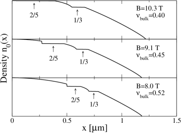
Figure 2: Equilibrium electronic densities $n_{0}(x)$ along a $1.2\,\mu$m edge for three values of magnetic field. The density falls from its bulk value $n_{b}=10^{11}\,\mathrm{cm}^{-2}$ to zero in each plot. Pictured are two incompressible stripes at $\nu=1/3$ and $\nu=2/5$. As the magnetic field increases, the bulk filling factor decreases and the incompressible stripes move move closer to the bulk. Here $d=30$ nm.

Given a particular confinement potential $W(x)$, we numerically solve Eq. (10) for the equilibrium density $n_{0}(x)$. An example using a parabolic edge confinement is shown in Fig. 2. Incompressible stripes of constant density are visible at FQHE fractions $\nu=2/5$ and $1/3$. The stripes vary with magnetic field: as the magnetic field increases the incompressible stripes move inward (toward the bulk), and new stripes appear at the outer edge. (To make the incompressible stripes more evident, we have used a smaller gate spacing $d=30$ nm in Fig. 2).

Now we can investigate the incompressible stripes’ effect on the edge magnetoplasmons. At each magnetic field we find $n_{0}(x)$ as outlined above, and then solve Eqs. (5) numerically for several values of $k$. Since our focus in this section is on the role of electronic structure we neglect dissipation (setting $\sigma_{xx}=0$ in Eq. (5a)); numerical solution of Eq. (5) is then straightforward. The results are similar to that of Ref. AG, , modified by the top gate and also by the different form of the equilibrium density. For each $k$ there are many modes. The fastest mode is always the nodeless mode. Since time-of-flight experiments are most sensitive to the fastest mode, we concentrate on it, finding a set of $k$-dependent mode densities $f(x)$ and eigenfrequencies $\omega$. An example is shown in Fig. 3. Notice that the mode density $f$ extends throughout the entire edge, dropping to zero at the position of an incompressible stripe but filling all of the compressible region. This is a consequence of the finite range of the interaction (5b), which reaches across the incompressible stripe.

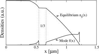
Figure 3: The equilibrium density $n_{0}(x)$ and the edge magnetoplasmon density $f(x)$ for the fastest mode, with $B=10.3\,\mathrm{T}$ ($\nu_{\mathrm{bulk}}=0.40$). The edge mode has a nonvanishing density only where the equilibrium density is compressible. Consequently $f(x)$ drops to zero along the incompressible $\nu=1/3$ stripe. The long-range Coulomb force couples all compressible regions.

In the long-wavelength limit the eigenfrequency $\omega\approx sk$ with $s$ the magnetoplasmon speed. By repeating the calculation with varying $B$ we find the mode speed as a function of magnetic field. Results in the FQHE regime are shown in Fig. 4. The speed falls generally as $1/B$, consistent with the classical result. Superimposed are small variations due to the spatial variation of the stripes with changing magnetic field. (As $\nu_{b}$ moves from just below to just above a FQHE fraction, a relatively large incompressible stripe shrinks abruptly into the bulk. This enlarges the compressible region and so diminishes the mode’s speed.)

It is evident in Fig. 4 that the $B$-dependence of the incompressible stripes has only a small influence on the edge magnetoplasmon’s speed. [In fact this is exaggerated in Fig. 4; for the purpose of illustration we (inconsistently) used $d=130$ nm in Eqs. 5 even though the equilibrium density $n_{0}(x)$ was calculated with $d=30$ nm. This gives a stronger restoring force and a larger variation in mode speed.] Within this semiclassical model, incompressible stripes do not lead to observable variations in speed.

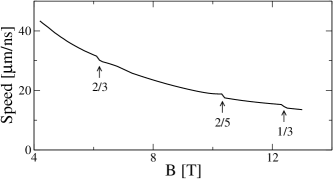
Figure 4: Speed of the fastest edge magnetoplasmon for the case shown in Figs. 2 and 3. The merging of incompressible stripes into the bulk produces small drops in speed.

IV Dissipation

In this section we examine how dissipation affects edge magnetoplasmons. We find that variations in dissipation due to the physics of the quantum Hall effect produce simultaneous variations in the edge mode’s speed and strength which should be observably large.

In the previous section we showed that incompressible stripes do not significantly influence the edge magnetoplasmons. Consequently in this section we use smooth edge density profiles, neglecting incompressible stripes. This lets us focus on the role of dissipation.

For orientation we begin with a simplified model which is analytically solvable, and which exhibits the effect of dissipation in a transparent way. This helps us disentangle the results of a numerical solution of the mode equations (5), which we will present last.

IV.1 Linear model

The model in question consists of: (i) taking the equilibrium edge density to be linear, and (ii) calculating the electric potential $\phi$ in the local capacitance approximation [Eq. (8)].

Write the equilibrium density as $n_{0}(x)=n_{b}\overline{n}(x)$ with

$$\overline{n}(x)=\left\{\begin{array}[]{ll}1&x\leq 0\\ 1-x/a&0\leq x\leq a.\end{array}\right.$$ (19)

Using this density profile, the local capacitance approximation Eq. (8), and the conductivities in Eq. (7), the mode equation [Eq. (5)] becomes

$$\frac{\omega}{\omega_{c}}\left[1-\left(\frac{\omega}{\omega_{c}}+\frac{i}{\omega_{c}\tau}\right)^{2}\right]f(x)=$$ (20)

$$\gamma a^{2}\left[-k\overline{n}^{\prime}f+\left(\frac{\omega}{\omega_{c}}+\frac{i}{\omega_{c}\tau}\right)\left(\overline{n}f^{\prime\prime}+\overline{n}^{\prime}f^{\prime}-k^{2}\overline{n}f\right)\right].$$

This is written to make the dimensional dependences clear. Here $\gamma$ is a dimensionless parameter:

$$\gamma=\frac{\ell_{0}d}{a^{2}},\mbox{\ with\ }\ell_{0}=\frac{4\pi e^{2}n_{b}}{\varepsilon m\omega_{c}^{2}}.$$ (21)

This introduces a new length scale $\ell_{0}$ which we will discuss shortly.

The mode equation Eq. (20) has an analytic solution. We will consider only long-wavelength modes, and hence drop the $k^{2}$ term. The solution of Eq. (20), given $\omega$, is

$$f(x)=\left\{\begin{array}[]{ll}Ae^{x/\lambda},&x<0\\ J_{0}\left(\xi\sqrt{1-x/a}\right),&0<x<a,\end{array}\right.$$ (22)

where

$$\lambda = a\sqrt{\displaystyle\frac{\gamma\omega_{c}^{2}(\omega+i/\tau)}{\omega[\omega_{c}^{2}-(\omega+i/\tau)^{2}]}},$$

$$\xi = 2\sqrt{\displaystyle\frac{ka\omega_{c}-\frac{\omega}{\gamma\omega_{c}^{2}}[\omega_{c}^{2}-(\omega+i/\tau)^{2}]}{\omega+i/\tau}}.$$ (23)

Here $A$ is an unknown constant. It and $\omega$ are fixed by matching $f$ and $f^{\prime}$ at $x=0$. The result is the secular equation

$$\frac{J_{0}(\xi)}{J_{1}(\xi)}=\sqrt{\displaystyle\frac{ka\gamma\omega_{c}^{3}/\omega}{\omega_{c}^{2}-(\omega+i/\tau)^{2}}-1}.$$ (24)

For each wave vector $k$ this has infinitely many solutions $\omega=\omega_{n}(k)$ giving the various edge magnetoplasmon modesAG . Notice that the exact eigenfrequencies have the symmetry $\omega_{n}(-k)=-\omega_{n}^{*}(k)$. Eq. (24) is consistent with this symmetry. Under $k\rightarrow-k$, $\xi\rightarrow\xi^{*}$ and both sides of Eq. (24) are complex conjugated.

We can obtain approximate solutions of the secular equation in the limiting cases $\gamma\ll 1$ and $\gamma\gg 1$. These correspond to, respectively, the limit of a very wide edge ($a\gg\sqrt{d\ell_{0}}$) and a narrow edge ($a\ll\sqrt{d\ell_{0}}$). Here we are comparing the edge width to a length given by the geometric mean of the gate spacing $d$ and the new length scale $\ell_{0}$ in Eq. (21). (This length scale $\ell_{0}$ also arose in Volkov and Mikhailov’s Wiener-Hopf treatment of semi-infinite systems with abrupt boundariesVM ). For a wide edge $a$ turns out to be much greater than the bulk penetration depth $\lambda$ and the edge mode resides primarily in the region $x>0$ where the equilibrium electronic density is nonuniform (see Fig. 1). Conversely for a narrow edge $a$ is much less than the penetration depth and the ‘edge mode’ resides primarily in the bulk (where it vanishes exponentially).

Using parameters for GaAs we can write $\ell_{0}$ from Eq. (21) in the equivalent forms

$$\ell_{0}=\frac{\nu_{b}\ell^{2}}{10\,\mbox{nm}}=\frac{66\nu_{b}}{\overline{B}}\,\mbox{nm},$$ (25)

where $\ell$ is the magnetic length, $\nu_{b}$ is the bulk filling factor, and $\overline{B}$ is the magnetic field in Tesla. A system with bulk density $n_{b}=10^{11}\,\mbox{cm}^{-2}$ achieves $\nu_{b}=1$ at $B=4.13\,\mbox{T}$, so that $\ell_{0}\approx 16\,\mbox{nm}$. In Ref. e2, $d\approx 130\,\mbox{nm}$, so $\sqrt{d\ell_{0}}\approx 50\,\mbox{nm}$. This is far smaller than the edge width $a\approx 500\,\mbox{nm}$, and so these experiments fall within the limiting case of a very wide edge ($\gamma\ll 1$).

IV.1.1 Narrow edge

First we consider the narow edge, for which $a\ll\sqrt{d\ell_{0}}$ and $\gamma\gg 1$. In this limit the edge mode lies largely in the bulk into which it exponentially decays.

When $\gamma\gg 1$ it turns out that the secular equation Eq. (24) is solved by $\xi\ll 1$. Replace the left-hand of Eq. (24) by the dominant term in the series expansion, $J_{0}(\xi)/J_{1}(\xi)\approx 2/\xi$. For large $\gamma$ the result is solved approximately by

$$\frac{\omega(k)}{\omega_{c}}=\sqrt{\frac{\ell_{0}dk^{2}}{1+1/(\omega_{c}\tau)^{2}}-\frac{1}{(2\omega_{c}\tau)^{2}}}-\frac{i}{2\omega_{c}\tau}$$ (26)

for $k>0$. [For $k<0$ use $\omega(-k)=-\omega(k)^{*}$.] Plugging this back into Eq. (21) yields $|\xi|\sim\gamma^{-1/4}$; this is small for large $\gamma$, consistent with our assertion above. The bulk penetration depth becomes approximately $|\lambda|\sim a\sqrt{\gamma}=\sqrt{d\ell_{0}}$, which here is much greater than the edge width $a$.

Eq. (26) is the dispersion relation of a single, dominant, mode in the limit of a narrow edge. It is pictured in Fig. 5. Only one mode appears because we kept only one term in the expansion of $J_{0}/J_{1}$. For small dissipation, the mode is underdamped for $k>1/2\omega_{c}\tau\sqrt{\ell_{0}d}$ and diffusive for smaller $k$. In the $k\to 0$ limit, we have $\omega(k)=-iDk^{2}$ where the diffusion constant is $D=s^{2}\tau$ and $s=\sqrt{\frac{4\pi e^{2}n_{b}d}{\varepsilon m}}$ is the velocity of the edge mode in the absence of dissipation (see below). The mode found here is closely connected to the result of Volkov and Mikhailov, who considered systems with $a$ identically zeroVM . Modifying their Wiener-Hopf technique to include a gate reproduces Eq. (26).

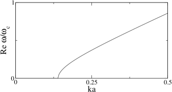
Figure 5: Model dispersion relation with a narrow edge. Here $1/\omega_{c}\tau=0.5$ , $\gamma=4$. Note that the solution is valid only for $|\omega/\omega_{c}|\ll 1$.

Notice an interesting aspect of the edge magnetoplasmon mode in this narrow edge regime: its velocity is nearly independent of magnetic field. For small dissipation, Eq. (26) becomes

$$\frac{\omega}{k}\approx\omega_{c}\sqrt{\ell_{0}d}=\sqrt{\frac{4\pi e^{2}n_{b}d}{\varepsilon m}}.$$ (27)

This behavior is quite different from that of wide edges, for which the velocity is largely $E/B$ drift. Here the mode resides mostly in the bulk (where it dies exponentially) and the electric field on the edge ($x>0$) plays no role.

Edge magnetoplasmons can be treated semiclassically only in the limit $a\gg\ell$, the case of a ‘smooth edge’ discussed in the introduction. The ‘narrow’ limit $a\ll\sqrt{d\ell_{0}}$ described in this section thus only gives physically reliable results when the magnetic length $\ell$ is much smaller than the other lengths $a$, $\sqrt{d\ell_{0}}$. To approach this narrow edge limit experimentally would require a combination of increased gate spacing $d$ and smaller electron density $n_{b}$ [the latter to increase $\ell_{0}$; see Eq. (21)]. Of course as a formal limit of the model described by Eq. (20) the limit always exists.

IV.1.2 Wide edge

The wide edge has $a\gg\sqrt{d\ell_{0}}$ and $\gamma\ll 1$. In this case there is little penetration into the bulk; the edge mode lives on the outer edge $x>0$ where the equilibrium density is inhomogeneous.

For orientation let us begin by removing the dissipation (set $1/\tau=0$). When $\gamma\ll 1$ it turns out that the right-hand side of Eq. (24) becomes small. (We check consistency below.) Consequently the solutions of Eq. (24) are given by

$$\xi\approx r_{n}$$ (28)

where $r_{n}\approx 2.405,5.520,\dots$ are the zeros of $J_{0}$ ($n=0,1,2,\dots$). Using Eq. (23) and (valid for long-wavelength modes) dropping terms second order in $\omega/\omega_{c}$, this gives

$$\omega_{n}(k)=\frac{\gamma\omega_{c}ka}{1+\gamma r_{n}^{2}/4}.$$ (29)

This is an example of the general results for nondissipative systems obtained by Aleiner and GlazmanAG . We see that that the fastest mode ($n=1$) is nodeless. Its speed is approximately $\gamma\omega_{c}a$, which is identical with the estimate Eq. (9); the speed falls as $1/B$.

Now turn on dissipation. We repeat the solution above, assuming that the right-hand side of Eq. (24) remains small; checking consistency at the end defines conditions (a lower bound on $ka$) under which this procedure gives an accurate solution. Combining Eqs. (23) and (28) yields

$$\omega_{n}(k)=\gamma\omega_{c}\,\frac{ka-\displaystyle\frac{r_{n}^{2}}{4}\frac{i}{\omega_{c}\tau}}{1+\gamma\displaystyle\frac{r_{n}^{2}}{4}-\left(\frac{\omega_{n}(k)}{\omega_{c}}+\frac{i}{\omega_{c}\tau}\right)^{2}}.$$ (30)

For small $\gamma$ this can be solved for $\omega_{n}(k)$ by iterative substitution into the denominator. For our purposes it is sufficient to look at the lowest order approximation,

$$\omega_{n}(k)=\gamma\omega_{c}\,\frac{ka-\displaystyle\frac{r_{n}^{2}}{4}\frac{i}{\omega_{c}\tau}}{1+\gamma\displaystyle\frac{r_{n}^{2}}{4}+\frac{1}{\omega_{c}^{2}\tau^{2}}}.$$ (31)

Once again we see the modes move slower as the number $n$ of nodes increases. It is also now evident that increasing $n$ leads to increasing damping ($|\mbox{Im}\,\omega_{n}|$ increases). Thus within this model the nodeless mode ($n=0$) is both the fastest and least damped, and will dominate time-of-flight experiments such as that of Ernst et al.

It remains to check consistency. Using Eq. (31), we find that the right-hand side of Eq. (24) is small as long as $ka\gg r_{n}^{2}/\omega_{c}\tau$. This regime exists for long-wavelength modes as long as the dissipation is sufficiently small. Then Eq. (31) is the dispersion relation for long wavelength modes above a lower bound ($ka\gg r_{n}^{2}/\omega_{c}\tau$). For such modes the bulk penetration depth $|\lambda|\approx a/(\omega_{c}\tau ka)^{1/2}$ is much less than $a$, as claimed; thus the mode resides largely on the outer edge.

The approximations leading to Eq. (31) fail for extremely long wavelengths ($ka\lesssim 1/\omega_{c}\tau$). Consider the limit $ka\ll 1/\omega_{c}\tau$. From Eq. (23) $\xi\ll 1$ and so $J_{0}(\xi)/J_{1}(\xi)\approx 2/\xi$. Then from Eq. (24) we find that at very long wavelenths the mode becomes diffusive: $\omega=-iDk^{2}$ with $D=\tau d4\pi e^{2}n_{b}/\varepsilon m$. Exactly the same diffusive limit occurs for small $k$ in the case of a narrow edge, from Eq. (26).

IV.2 Oscillations in the quantum Hall regime

Our last step is to model the variation of the dissipation with magnetic field and to show how this variation influences the edge magnetoplasmons. As disucssed in Section II, we treat $1/\tau$ as a global property of the edge which depends only on the bulk filling factor $\nu_{b}$. This incorporates one crucial aspect of quantum mechanics (the loss of dissipation on a Hall plateau) into an otherwise classical treatment of edge magnetoplasmons. We expect this to at least qualitatively capture the role of dissipation for the edge magnetoplasmons. It turns out that the effect is appreciable.

We model the magnetic field dependence of $1/\tau$ in the following manner:

$$\frac{1}{\omega_{c}\tau}=\left(\frac{1}{\omega_{c}\tau}\right)_{\mathrm{max}}g(\nu_{b}).$$ (32)

Here $g(\nu_{b})$ is a function which is zero on Hall plateaus and rises to a maximum value of 1 between plateaus. In such a phenomenological model one can include as many Hall plateaus as desired. In the following we keep Hall plateaus at $\nu_{b}=2,1,2/3,1/3$. The detailed shape of $g(\nu_{b})$ is unimportant. For convenience we used a Gaussian, pictured in Fig. 6. At typical experimental temperatures the constant $(1/\omega_{c}\tau)_{\mathrm{max}}$ should be of order 1.

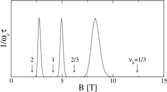
Figure 6: Model for $1/\omega_{c}\tau$. The peak value between Hall plateaus is $(1/\omega_{c}\tau)_{\mathrm{max}}$.

Switching on the dissipation $1/\omega_{c}\tau$ between Hall plateaus both damps the edge magnetoplasmons and changes their speed. For example, for a wide edge consider the model dispersion relation in Eq. (31). Between Hall plateaus $\mathrm{Im}\,\omega_{n}(k)$ becomes nonzero and the mode is damped. At the same time $\mathrm{Re}\,\omega_{n}(k)$ gets smaller — the mode slows down as it is damped. Thus switching on and off the dissipation as the system moves off and on Hall plateaus causes simultaneous oscillations in the mode speed and strength. The strength of the oscillations grows with $(1/\omega_{c}\tau)_{\mathrm{max}}$ and can be appreciable (see the next section).

The oscillations could be quite large for a narrow edge. In a time-of-flight experiment an initial voltage pulse triggers an electron density pulse which travels along the edge. Suppose the density pulse is a wave packet centered around a characteristic wave vector $k_{0}$. For small dissipation, modes near $k_{0}$ will be underdamped and move with a speed of order $\omega_{c}\sqrt{\ell_{0}d}$ [see Eqs. (26, 27)]. As the dissipation grows the modes near $k_{0}$ can become diffusive, yielding large drops in signal strength and velocity.

In the next section we examine the role of dissipation on the edge magnetoplasmons with fewer approximations, continuing to use the phenomenological model for dissipation [Eq. (32)], but solving the mode equations [Eqs. (5)] numerically.

IV.3 Dissipation and edge modes: numerical results

We conclude by studying the effect of dissipation on the edge magnetoplasmons by direct numerical solution of Eqs. (5). The simplest way to do this is to discretize space, which converts the mode equations into an eigenvalue problem. Since the resulting matrix to be diagonalized is complex, some care needs to be taken in identifying the proper modes. We were guided by the analytical results obtained above.

In this section we use parameters similar to the experiments of Ref. e2, . Here the bulk electronic density $n_{b}=10^{11}\,\mathrm{cm}^{-2}$, the gate spacing $d=130\,\mathrm{nm}$, edge width $a=1.2\,\mu\mathrm{m}$, and for GaAs $m=0.067\,\mathrm{m}_{e}$, $\varepsilon=12.4$. As mentioned above, these parameters put us well within the limit of wide edges. The modes are not very sensitive to the details of the edge confinement. Here we use a parabolic confinement; this leads to an edge density profile $n_{0}(x)=n_{b}(1-x^{2}/a^{2})$ for $0<x<a$. Because $|\omega|\ll\omega_{c}$ for the fields considered it was sufficient to take the DC limit of the conductivities Eq. (7). The mode equations are solved for the eigenvalues $\omega$ and corresponding mode densities $f(x)$ as a function of $B$ and $k$.

Diagonalization of the discretized form of Eqs. (5) yields as many modes as there are grid points (typically 200-500). In the presence of dissipation the eigenvalues become complex. An example is pictured in Fig. 7, which shows the 12 eigenvalues with the smallest dissipation for a particular run. Notice that one mode in Fig. 7 is singled out as both the fastest and least damped. This mode dominates time-of-flight experiments. As the dissipation increases this mode continues to be identifiable; the fastest mode continues to have relatively small damping. In the following we focus on this dominant mode.

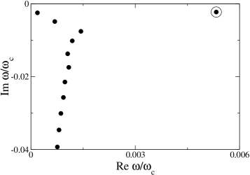
Figure 7: Eigenvalues in the presence of dissipation. Pictured are the 12 eigenvalues with the smallest $|\mathrm{Im}\,\omega|$. Notice that one mode (circled) is both the fastest and least damped. This is the dominant mode for time-of-flight experiments. Here $\nu_{b}=1.5$, $(1/\omega_{c}\tau)_{\mathrm{max}}=0.3$, $k=1/a$.

In the absence of dissipation the dominant mode resides entirely on the edge. Switching on dissipation causes it to penetrate into the bulk, where it dies exponentially (Fig. 8).

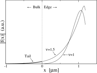
Figure 8: Mode densities for $\nu_{b}=1$ and $\nu_{b}=1.5$. In the absence of dissipation ($\nu_{b}=1$) the mode resides entirely on the edge. In the presence of dissipation ($\nu_{b}=1.5$) the mode has an exponentially decreasing tail in the bulk. Here $(1/\omega_{c}\tau)_{\mathrm{max}}=0.05$, $k=1/a$.

Sweeping the wave vector $k$ yields a dispersion relation $\omega(k)$ for the dominant mode. This is pictured for two cases (no dissipation at $\nu_{b}=1$, dissipation at $\nu_{b}=1.5$) in Fig. 9.

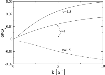
Figure 9: Dispersion relation $\omega(k)$ for the dominant mode for a nondissipative case ($\nu=1$) and a dissipative case ($\nu=1.5$). The solid lines are $\mathrm{Re}\,\omega$ and the broken lines are $\mathrm{Im}\,\omega$. For very small $k$ in the presence of dissipation the mode becomes diffusive and difficult to identify within the numerical results. Here $(1/\omega_{c}\tau)_{\mathrm{max}}=0.3$.

The speed and damping of the dominant mode as a function of magnetic field are shown in Fig. 10. In a time-of-flight experiment wave packets centered at some $k_{0}$ travel along the edge. The value of $k_{0}$ is set by geometrical factors (such as the probe dimensions) and the time dependence of the voltage pulse. Typically a voltage probe is about a micron wide and is also about a micron from the edge of the electronic system. This is approximately the size of the edge width $a$. Consequently we assume that $k_{0}$ is of order $1/a$. (The results below do not change qualitatively as long as $k_{0}$ is in the linear portion of the dispersion relation for small dissipation.) The speed shown in the upper panel of Fig. 10 is the slope

$$s=\left.\frac{d\omega}{dk}\right|_{k=k_{0}}~{},$$ (33)

where $k_{0}=1/a$. Superimposed on the $1/B$ trend in velocity are oscillations caused by switching on dissipation between plateaus. We report the mode’s strength using an inverse decay length

$$\eta^{-1}=|\mathrm{Im}\,\omega(k_{0})|/s.$$ (34)

In the absence of dissipation $\eta^{-1}=0$. Increasing dissipation leads to increasing $\eta^{-1}$, as shown in the lower panel of Fig. 10.

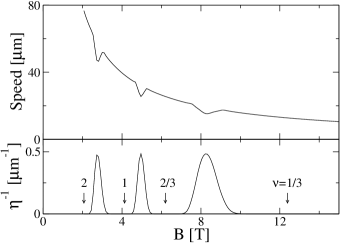
Figure 10: Speed and damping of the fastest mode as a function of magnetic field. Increasing dissipation between Hall plateaus leads to more damping (shown in the lower panel as an inverse decay length) and oscillations in speed (shown in the upper panel). Here $(1/\omega_{c}\tau)_{\mathrm{max}}=1$.

The oscillations in speed and damping evident in Fig. 10 are large enough to be experimentally visible. They are at least qualitatively similar to the oscillations in signal strength and mode speed observed in the experiments of Ernst et al.,e2 and may explain their results.

V Summary

We have presented a semiclassical treatment of edge magnetoplasmons in the quantum Hall regime, in the presence of dissipation. Our treatment of the edge magnetoplasmons is essentially classical, with dynamics arising from the continuity equation and self-consistent electric fields. Quantum mechanics enters the calculation in two places. First, energy gaps associated with the quantum Hall effect lead to incompressible stripes within the largely incompressible edge. We find these stripes to have very little effect on the edge modes. But the physics of the quantum Hall effect also enters in a second place, as a dissipative contribution to the conductivity tensor. The dissipation influences the modes in a natural way. Between Hall plateaus, switching on dissipation leads to increased damping and a diminished mode velocity. This behavior is similar to the expected role of dissipation in other signatures of electronic plasma oscillations, such as Surface Acoustic Wave (SAW) experiments. The interesting aspect of quantum Hall effect systems is that the dissipation can be turned on and off by varying the magnetic field.

- (1) See, for example, The Quantum Hall Effect, ed. by R.E. Prange and S.M. Girvin, Springer-Verlag (New York), 1990.
- (2) G. Ernst, R.J. Haug, J. Kuhl, K. v. Klitzing, and K. Eberl, Phys. Rev. Lett. 77, 4245 (1996).
- (3) G.B. Ernst, N.B. Zhitenev, R.J. Haug, and K. von Klitzing, Phys. Rev. Lett. 79, 3748 (1997); Physica E 1, 95 (1998).
- (4) Gabriele Ernst, Zeitaufgel ste Transportmessungen zum Quanten-Hall-Effekt (Ph.D. thesis, Universität Stuttgart, Feb. 1997); and private communication.
- (5) R.C. Ashoori et al., Phys. Rev. B 45, 3894 (1992).
- (6) U. Zülicke, A.H. MacDonald, and M.D. Johnson, Phys. Rev. B 58, 13778 (1998).
- (7) A.M. Chang, L.N. Pfeiffer and K.W. West, Phys. Rev. Lett. 77, 2538 (1996).
- (8) X.G. Wen, Phys. Rev. B 41, 12838 (1990); Phys. Rev. B 44, 5708 (1991); Phys. Rev. Lett. 64, 2206 (1990).
- (9) M. Stone, Annals of Physics 207, 38 (1991).
- (10) C.L. Kane and M.P.A. Fisher, Phys. Rev. B 51, 13449 (1995).
- (11) J.J. Palacios and A.H. MacDonald, Phys. Rev. Lett. 76, 118 (1996).
- (12) A.V. Shytov, L.S. Levitov, and B.I. Halperin, Phys. Rev. Lett. 80, 141 (1998).
- (13) F.P. Milliken, C.P. Umbach and R.A. Webb, Solid State Comm. 97, 309 (1996).
- (14) M. Grayson et al., Phys. Rev. Lett. 80, 1062 (1998).
- (15) S. Conti and G. Vignale, “Bosonization of the two-dimensional electron gas in the lowest Landau level,” preprint cond-mat/9801318.
- (16) U. Zülicke and A.H. MacDonald, Phys. Rev. B 60, 1837-1841 (1999).
- (17) D.H. Lee and X.G. Wen, “Edge tunneling in fractional quantum Hall regime,” preprint cond-mat/9809160.
- (18) L.S. Levitov, A.V. Shytov, and B.I. Halperin, Phys. Rev. B 64, 75322 (2001).
- (19) M. Grayson et al., Phys. Rev. Lett. 86, 2645 (2001).
- (20) C.W.J. Beenakker, Phys. Rev. Lett. 64, 216 (1990).
- (21) D.B. Chklovskii, B.I. Shklovskii, and L.I. Glazman, Phys. Rev. B 46, 4026 (1992).
- (22) V.A. Volkov and S.A. Mikhailov, Zh. Eksp. Teor. Fiz. 94, 217 (1988) [Sov. Phys. JETP 67, 1639 (1988)].
- (23) I.L. Aleiner and L.I. Glazman, Phys. Rev. Lett. 72, 2935 (1994); I.L. Aleiner, D. Yue , and L.I. Glazman, Phys. Rev. B 51, 13467 (1995).
- (24) N.B. Zhitenev, R.J. Haug, K. v. Klitzing, and K. Eberl, Phys. Rev. B 52, 11277 (1995).
- (25) M.I. Lubin, O. Heinonen, and M.D. Johnson, Phys. Rev. B 56, 10373 (1997).