Anomalous diffusion and collapse of self-gravitating
Langevin particles in $D$ dimensions

Abstract

We address the generalized thermodynamics and the collapse of a system of self-gravitating Langevin particles exhibiting anomalous diffusion in a space of dimension $D$. This is a basic model of stochastic particles in interaction. The equilibrium states correspond to polytropic configurations similar to stellar polytropes and polytropic stars. The index $n$ of the polytrope is related to the exponent of anomalous diffusion. We consider a high-friction limit and reduce the problem to the study of the nonlinear Smoluchowski-Poisson system. We show that the associated Lyapunov functional is the Tsallis free energy. We discuss in detail the equilibrium phase diagram of self-gravitating polytropes as a function of $D$ and $n$ and determine their stability by using turning points arguments and analytical methods. When no equilibrium state exists, we investigate self-similar solutions of the nonlinear Smoluchowski-Poisson system describing the collapse. Our stability analysis of polytropic spheres can be used to settle the generalized thermodynamical stability of self-gravitating Langevin particles as well as the nonlinear dynamical stability of stellar polytropes, polytropic stars and polytropic vortices.

1 Introduction

In preceding papers of this series [1, 2, 3, 4], we have studied a model of self-gravitating Brownian particles enclosed within a spherical box of radius $R$ in a space of dimension $D$. This model can be considered as a prototypical dynamical model of systems with long-range interactions possessing a rich thermodynamical structure. For simplicity, we considered the Smoluchowski-Poisson (SP) system which is deduced from the Kramers-Poisson (KP) system in a high friction limit (or for large times). These Fokker-Planck-Poisson equations were first proposed in [1] as a simplified dynamical model of self-gravitating systems. Their relation with thermodynamics (first and second principles) was clearly established in terms of a maximum entropy production principle (MEPP) and their rich properties (self-organized states or collapse) were described qualitatively in this preliminary work. A thorough study of this system of equations was undertaken more recently in [2, 3, 4], complemented by rigorous mathematical results (see [5, 6, 7, 8, 9] and references therein).

The Smoluchowski equation is a particular Fokker-Planck equation involving a diffusion and a drift [10]. In our model, the drift is directed toward the region of high densities due to the gravitational force which is generated by the particles themselves. This retroaction leads to a situation of collapse when attraction prevails over diffusion [2, 3, 4]. The SP system also provides a simplified model for the chemotactic aggregation of bacterial populations [11] and for the formation of large-scale vortices in two-dimensional hydrodynamics [12, 13, 14, 15, 16, 17]. It can be shown that the SP system decreases continuously a free energy constructed with the Boltzmann entropy [1, 2]. Accordingly, the stationary solutions of the SP system are given by the Boltzmann distribution which minimizes Boltzmann’s free energy at fixed mass. The equilibrium state is then determined by solving the Boltzmann-Poisson (or Emden) equation, as in the case of isothermal gaseous stars and isothermal stellar systems [18, 19]. However, depending on the value of the temperature $T$, an equilibrium solution does not always exist and the system can undergo a catastrophic collapse. We determined analytically and numerically self-similar solutions leading to a finite time singularity [2, 3]. In [3, 4], we showed that the evolution continues after the collapse until a Dirac peak is formed.

In this paper, we propose to extend our study to a generalized class of Smoluchowski equations [20]. They can be obtained from the familiar Smoluchowski equation by assuming that the diffusion coefficient depends on the density while the drift coefficient is constant (or the opposite). They can also be obtained from standard stochastic processes by considering a special form of multiplicative noise [21, 20] or an extended class of transition probabilities [22, 23]. These equations are consistent with a generalized maximum entropy production principle [20]. For simplicity, we shall assume that the diffusion coefficient is a power law of the density. In the absence of drift, this would lead to anomalous diffusion. If we take into account a drift term and a self-attraction, we have to solve the nonlinear Smoluchowski-Poisson (NSP) system. It can be shown [20, 24] that the NSP system decreases continuously a free energy associated with Tsallis entropy [25]. Accordingly, the stationary solutions of the NSP system are given by a polytropic distribution which minimizes Tsallis’ free energy at fixed mass. The equilibrium state is then determined by solving the Lane-Emden equation, as in the case of polytropic stars and stellar polytropes [18, 19]. Depending on the value of the control parameter and on the index $n$ of the polytrope, three situations can occur: (i) the NSP system can relax toward an incomplete polytrope maintained by the walls of the confining box (ii) the NSP system can relax toward a stable complete polytrope of radius $R_{*}<R$, unaffected by the box (iii) the NSP system can undergo a catastrophic collapse leading to a finite time singularity.

The paper has two parts that are relatively independent. In the first part of the paper (Secs. 2 and 3), we study the dynamical stability of stellar systems, gaseous stars and two-dimensional (2D) vortices by using a thermodynamical analogy [26, 20, 23]. Stellar polytropes maximize Tsallis entropy (considered as a $H$-function) at fixed mass and energy. This is a condition of nonlinear dynamical stability via the Vlasov equation. Polytropic stars minimize Tsallis free energy (related to the star energy functional) at fixed mass. This is a condition of nonlinear dynamical stability via the Euler-Jeans equations. Polytropic vortices maximize Tsallis entropy (considered as a $H$-function) at fixed circulation and energy. This is a condition of nonlinear dynamical stability via the 2D Euler equation. We perform an exhaustive study of the structure and stability of polytropic spheres by determining whether they are maxima or minima (or saddle points) of Tsallis functional. For sake of generality, we perform our study in a space of dimension $D$. We shall exhibit particular dimensions $D=2$, $D=4$, $D=2(1+\sqrt{2})$ and $D=10$ which play a special role in our problem. The dimension $D=2$ is critical because the results established for $D>2$ cannot be directly extended to $D=2$ [3]. On the other hand, the nature of the caloric curve changes for $D=4$ and $D=10$. This extends the study performed by Taruya & Sakagami [27, 28] and Chavanis [29, 26] for $D=3$.

In the second part of the paper (Sec. 4), we study the dynamics and thermodynamics of self-gravitating Langevin particles experiencing anomalous diffusion. Their equilibrium distribution minimizes Tsallis free energy at fixed mass. This is a condition of thermodynamical stability in a generalized sense. This is also a condition of linear dynamical stability via generalized Fokker-Planck equations (in the present context the NSP system)[2, 24, 20]. Thus, the stability analysis of Sec. 3 can also be used in that context. When the static solution does not exist or is unstable, the system undergoes a catastrophic collapse. In Sec. 4, we show that the NSP system admits self-similar solutions describing the collapse and leading to a finite time singularity. The density decreases at large distances as $\rho\sim r^{-\alpha}$. In the canonical situation (fixed $T$), the scaling exponent is $\alpha_{n}=2n/(n-1)$ where $n$ is the polytropic index. We also consider a microcanonical situation in which the generalized temperature $T(t)$ varies in time so as to rigorously conserve energy. In that case, the scaling equation has solutions for $\alpha_{n}\leq\alpha\leq\alpha_{\rm max}(n,D)$ where $\alpha_{\rm max}(n,D)$ is a non-trivial exponent. The value of $\alpha$ effectively selected by the system is determined by the dynamics. In Sec. 5, we perform direct numerical simulations of the SP and NSP systems with higher accuracy than in Ref. [2]. We confirm the scaling regime and discuss the value of the scaling exponent. In the microcanonical situation, we give numerical evidence that $\alpha=\alpha_{n}$ so that the temperature $T(t)$ is finite at the collapse time (this observation has been made independently by [9] for the SP system). However, the convergence to this value is so slow that the evolution displays a pseudo-scaling regime with $\alpha_{n}\leq\alpha\leq\alpha_{\rm max}$ for the densities achieved. We explain the physical reason for this behavior and we conjecture that $\alpha\simeq\alpha_{\rm max}$ will be reached in more realistic models with non-uniform temperature [30]. This paper closely follows the style and presentation of our companion paper for isothermal spheres [3]. These two papers complete the classical monograph of Chandrasekhar on self-gravitating isothermal and polytropic spheres in $D=3$ [18].

2 Dynamical stability of systems with long-range interactions

2.1 Stellar systems

Let us consider a collection of $N$ stars with mass $m$ in gravitational interaction. They form a Hamiltonian $N$-body system with long-range (Newtonian) interactions. We work in a space of dimension $D$ and enclose the system within a spherical box of radius $R$. Let $f({\bf r},{\bf v},t)$ denote the distribution function of the system, i.e. $f({\bf r},{\bf v},t)d^{D}{\bf r}d^{D}{\bf v}$ gives the mass of stars whose position and velocity are in the cell $({\bf r},{\bf v};{\bf r}+d^{D}{\bf r},{\bf v}+d^{D}{\bf v})$ at time $t$. The integral of $f$ over the velocity determines the spatial density

(1) $$\rho=\int f\,d^{D}{\bf v}.$$

The total mass of the configuration is

(2) $$M=\int\rho\,d^{D}{\bf r}.$$

In the mean-field approximation, the total energy of the system can be expressed as

(3) $$E={1\over 2}\int fv^{2}\,d^{D}{\bf r}d^{D}{\bf v}+{1\over 2}\int\rho\Phi\,d^{D}{\bf r}=K+W,$$

where $K$ is the kinetic energy and $W$ the potential energy. The gravitational potential $\Phi$ is related to the density by the Newton-Poisson equation

(4) $$\Delta\Phi=S_{D}G\rho,$$

where $S_{D}$ is the surface of a unit sphere in a $D$-dimensional space and $G$ is the constant of gravity.

For fixed $N\gg 1$ and $t\rightarrow+\infty$, the system is expected to reach a statistical equilibrium state described by the classical Boltzmann entropy $S_{B}[f]=-\int f\ln fd^{D}{\bf r}d^{D}{\bf v}$. However, the relaxation time $t_{relax}$ due to “collisions” (more properly close encounters) is in general considerably larger than the dynamical time $t_{D}$ so that this statistical equilibrium state is often not physically relevant [31, 32]. This is the case in particular for elliptical galaxies where $t_{relax}\sim{N\over\ln N}t_{D}$ with $N\sim 10^{12}$, while their age is $\sim 100t_{D}$ [19]. For $t\ll t_{relax}$ and $N\rightarrow+\infty$, the dynamics of stars is described by the Vlasov equation

(5) $${\partial f\over\partial t}+{\bf v}{\partial f\over\partial{\bf r}}+{\bf F}{\partial f\over\partial{\bf v}}=0,$$

where ${\bf F}=-\nabla\Phi$ is the gravitational force determined by the Poisson equation (4). For any $H$-function

(6) $$S[f]=-\int C(f)d^{D}{\bf r}d^{D}{\bf v},$$

where $C$ is convex, i.e. $C^{\prime\prime}>0$, it can be shown that the variational problem

(7) $${\rm Max}\quad S[f]\quad{\rm at\ fixed}\quad E[f],M[f],$$

determines a stationary solution of the Vlasov equation with strong (nonlinear) dynamical stability properties [33, 34]. Such solutions can result from a process of (possibly incomplete) violent relaxation [26]. Introducing Lagrange multipliers, the first order variations $\delta S-\beta\delta E-\alpha\delta M=0$ lead to

(8) $$C^{\prime}(f)=-\beta\biggl{(}{v^{2}\over 2}+\Phi\biggr{)}-\alpha.$$

Therefore, $f=f(\epsilon)$ where $\epsilon={v^{2}\over 2}+\Phi$ is the energy of a star by unit of mass. These distribution functions, depending only on the energy, form a particular class of stationary solutions of the Vlasov equation. Other solutions can be constructed with the Jeans theorem [19] but their stability is more difficult to investigate. The conservation of angular momentum can be easily included in the foregoing discussion [35].

2.2 Barotropic stars

Let us now consider a self-gravitating gaseous system described by the Euler-Jeans equations

(9) $${\partial\rho\over\partial t}+\nabla(\rho{\bf u})=0,$$

(10) $${\partial{\bf u}\over\partial t}+({\bf u}\cdot\nabla){\bf u}=-{1\over\rho}\nabla p-\nabla\Phi.$$

We assume that the gas is barotropic with an equation of state $p=p(\rho)$. The most important examples of barotropic fluids are those that are isentropic or adiabatic, that is those whose specific entropy is constant. If $s={\rm Cst.}$, the first principle of thermodynamics $du=-pdv+Tds$ (where $v=1/\rho$) reduces to $du={p\over\rho^{2}}d\rho$, where $u$ is the internal energy by unit of mass. The total energy of the fluid is therefore

(11) $${\cal W}[\rho]=\int\rho\int_{0}^{\rho}{p(\rho^{\prime})\over\rho^{{}^{\prime}2}}d\rho^{\prime}d^{D}{\bf r}+{1\over 2}\int\rho\Phi d^{D}{\bf r}+\int\rho{{\bf u}^{2}\over 2}d^{D}{\bf r}.$$

The first term is the internal energy, the second the gravitational energy and the third the kinetic energy associated with the mean motion. As argued in [26], the variational problem

(12) $${\rm Min}\quad{\cal W}[\rho]\quad{\rm at\ fixed}\quad M[\rho],$$

determines a stationary solution of the Euler-Jeans equations with strong (nonlinear) dynamical stability properties. We shall not prove this result here but it is expected to follow from relatively standard methods of stability theory. The solutions of this variational problem satisfy the condition of hydrostatic balance

(13) $$\nabla p=-\rho\nabla\Phi,$$

between pressure and gravity. The foregoing results can be extended to barotropic stars rotating rigidly with angular velocity $\Omega$$\Omega$$\Omega$ [35].

2.3 Two-dimensional vortices

Let us finally consider a collection of $N$ point vortices with circulation $\gamma$ in 2D hydrodynamics. They form a Hamiltonian system with long-range (logarithmic) interactions. We call $\omega$ the vorticity, $\psi$ the stream function and ${\bf u}=-{\bf z}{\times}\nabla\psi$ the velocity field. We also note $\Gamma=\int\omega d^{2}{\bf r}$ the circulation and $E={1\over 2}\int\omega\psi d^{2}{\bf r}$ the energy. For fixed $N\gg 1$ and $t\rightarrow+\infty$, the system is expected to reach a statistical equilibrium state described by the classical Boltzmann entropy $S_{B}[\omega]=-\int\omega\ln\omega d^{2}{\bf r}$ [36]. However, the relaxation time $t_{relax}$ due to “collisions” is in general considerably larger than the dynamical time $t_{D}$ so that this statistical equilibrium state is often not physically relevant [15, 16]. For $t\ll t_{relax}$ and $N\rightarrow+\infty$, the dynamics of point vortices is described by the 2D Euler-Poisson system

(14) $${\partial\omega\over\partial t}+{\bf u}\cdot\nabla\omega=0,$$

(15) $$\omega=-\Delta\psi.$$

The Euler equation also governs the dynamics of 2D incompressible and inviscid continuous vorticity fields. For any $H$-function

(16) $$S[\omega]=-\int C(\omega)d^{2}{\bf r},$$

where $C$ is convex, i.e. $C^{\prime\prime}>0$, it can be shown that the variational problem

(17) $${\rm Max}\quad S[\omega]\quad{\rm at\ fixed}\quad E[\omega],\Gamma[\omega],$$

determines a stationary solution of the 2D Euler equation with strong (nonlinear) dynamical stability properties [37]. Such solutions can result from a process of (possibly incomplete) violent relaxation [17]. Introducing Lagrange multipliers, the condition $\delta S-\beta\delta E-\alpha\delta\Gamma=0$ leads to

(18) $$C^{\prime}(\omega)=-\beta\psi-\alpha.$$

Therefore, $\omega=\omega(\psi)$, which is the general form of stationary solutions of the 2D Euler equation for domains with no specific symmetries. The conservation of angular momentum and impulse can be easily included in the foregoing discussion [20].

2.4 Thermodynamical analogy

Since the variational problems (7), (12) and (17) are similar to the usual variational problems that arise in thermodynamics (with the Boltzmann entropy), we can develop a thermodynamical analogy to analyze the dynamical stability of stellar systems, gaseous stars and 2D vortices [26, 20, 23, 17]. In this analogy, the functional $S$ plays the role of a generalized entropy, $\beta$ is a generalized inverse temperature, $\beta(E)$ a generalized caloric curve etc… The variational problem (7) is similar to a condition of microcanonical stability. We can also introduce a generalized free energy $F[f]=E[f]-TS[f]$ which is the Legendre transform of $S[f]$. The minimization of $F[f]$ at fixed $T$ and $M[f]$ is similar to a condition of canonical stability. This is equivalent to first minimize $F[f]$ at fixed $\rho({\bf r})$ to get $f_{*}({\bf r},{\bf v})$ and then to minimize $F[\rho]=F[f_{*}]$, calculated with $f_{*}$, at fixed $M[\rho]$. Now, it can be shown [26] that $F[\rho]$ is precisely the functional (11) with ${\bf u}={\bf 0}$. Therefore, the variational problem (12) is similar to a condition of canonical stability. Since canonical stability implies microcanonical stability (but not the converse) [20], we conclude that “stellar systems are stable whenever corresponding barotropic stars are stable” which provides a new interpretation of Antonov’s first law [26].

In 2D hydrodynamics, the variational problem (17) is similar to a condition of microcanonical stability. It is stronger than the maximization of $J[\omega]=S[\omega]-\beta E[\omega]$ at fixed $\beta$ and $\Gamma[\omega]$ (canonical stability), which is just a sufficient condition of nonlinear dynamical stability. It is not a necessary condition of stability if the ensembles are inequivalent (i.e. if the “caloric curve” presents bifurcations or turning points). The Arnold’s theorems just provide sufficient conditions of canonical stability (see, e.g., [20]). Therefore, in the domain of inequivalence (corresponding to a region of “negative specific heats”) a flow can be nonlinearly dynamically stable while it violates Arnold’s theorems. This has important implications in jovian fluid dynamics [37, 38].

The preceding arguments also apply to other systems with long-range interactions such as the HMF model for example [39]. This opens the route to many generalizations by changing the potential of interaction and the “generalized entropy” (H-function). In this paper, we shall specialize in the case of particles interacting via a Newtonian potential (e.g., self-gravitating systems, 2D vortices,…). We shall also consider a special form of $H$-function, known as Tsallis entropy, leading to power-laws distributions (polytropes).

3 Equilibrium structure of polytropic spheres in dimension $D$

3.1 Stellar polytropes

Let us consider a particular class of stationary solutions of the Vlasov equation called stellar polytropes [19]. Nonlinearly dynamically stable solutions maximize the Tsallis entropy

(19) $$S_{q}=-{1\over q-1}\int(f^{q}-f)\,d^{D}{\bf r}d^{D}{\bf v},$$

at fixed mass $M$ and energy $E$, where $q$ is a real number. For $q\rightarrow 1$, Eq. (19) reduces to the ordinary Boltzmann entropy describing isothermal stellar systems. We emphasize that, in the present context, Tsallis and Boltzmann entropies are particular $H$-functions (not true entropies) that are related to the dynamics, not to the thermodynamics. Still, due to the thermodynamical analogy discussed in Sec. 2.4, we shall use a thermodynamical langage to study the dynamical stability problem. In this analogy, the dynamical stability criterion for stellar polytropes corresponds to a microcanonical stability condition.

The critical points of entropy at fixed mass and energy satisfy the condition

(20) $$\delta S_{q}-\beta\delta E-\lambda\delta M=0,$$

where $\beta=1/T$ and $\lambda$ are Lagrange multipliers ($T$ is the temperature and $\lambda$ the chemical potential in the generalized sense). The variational principle (20) leads to the polytropic distribution function

(21) $$f({\bf r},{\bf v})=\biggl{\{}\mu-{(q-1)\beta\over q}\biggl{[}{v^{2}\over 2}+\Phi({\bf r})\biggr{]}\biggr{\}}^{1\over q-1},$$

where $\mu=[1-(q-1)\lambda]/q$. We define the polytropic index $n$ by the relation

(22) $$n={D\over 2}+{1\over q-1}.$$

We first consider the case $(q-1)\beta/q>0$ and allow $\beta$ to take negative values. Then, Eq. (21) can be rewritten

(23) $$f=A\biggl{[}\alpha-\Phi-{v^{2}\over 2}\biggr{]}^{n-{D\over 2}},$$

where

(24) $$A=\biggl{[}{(q-1)\beta\over q}\biggr{]}^{1\over q-1},\qquad\alpha={1-(q-1)\lambda\over(q-1)\beta}.$$

If $n>D/2$ (i.e., $q>1$ and $\beta>0$), $f^{\prime}(\epsilon)<0$ where $\epsilon={v^{2}\over 2}+\Phi$ is the stellar energy. Therefore, high energy particles are less probable than low energy particles, which corresponds to the physical situation. Equation (23) is valid for $v<v_{max}=\sqrt{2(\alpha-\Phi)}$. If $v>v_{max}=\sqrt{2(\alpha-\Phi)}$, we set $f=0$. This distribution function describes stellar polytropes which were first introduced by Plummer [40]. If $n=D/2$ (i.e., $q\rightarrow\infty$), the distribution $f(\epsilon)$ is a step function. This corresponds to the self-gravitating Fermi gas at zero temperature (white dwarfs). In $D=3$, classical white dwarf stars are equivalent to polytropes with index $n=3/2$ [18]. In $D$-dimensions, classical “white dwarf stars” are equivalent to polytropes with index

(25) $$n_{3/2}={D\over 2}.$$

If $n\rightarrow+\infty$ (i.e. $q\rightarrow 1$), we recover isothermal distibution functions. If $n<D/2$ (i.e., $q<1$ and $q\beta<0$), high energy particles are more probable than low energy particles: $f^{\prime}(\epsilon)>0$. This situation is unphysical but it can be considered at a formal level. The distribution function diverges like $(1-v/v_{max})^{n-D/2}$ as $v\rightarrow v_{max}$. The moments of $f$ converge if and only if $n>D/2-1$. Therefore, if $D/2-1<n<D/2$ (i.e., $q<0$ and $\beta>0$), stellar polytropes exist mathematically but they are not physical. If $n<D/2-1$ (i.e., $0<q<1$ and $\beta<0$), stellar polytropes do not exist.

We now consider the case $(q-1)\beta/q<0$. Then, Eq. (21) can be rewritten

(26) $$f=A\biggl{[}\alpha+\Phi+{v^{2}\over 2}\biggr{]}^{n-{D\over 2}},$$

where

(27) $$A=\biggl{[}{(1-q)\beta\over q}\biggr{]}^{1\over q-1},\qquad\alpha={1-(q-1)\lambda\over(1-q)\beta}.$$

If $n>D/2$ (i.e., $q>1$ and $\beta<0$), the model is ill-posed because $f(v)$ diverges for $v\rightarrow+\infty$. If $n<D/2$, the distribution function goes to zero like $v^{-(D-2n)}$ for $v\rightarrow+\infty$. If $0<n<D/2$ (i.e., $q<1-2/D$), the density $\rho=\int fd^{D}{\bf v}$ does not exist. If $-1<n<0$ (i.e., $1-2/D<q<D/(D+2)$), the density exists but not the pressure $p={1\over D}\int fv^{2}d^{D}{\bf v}$. If $n<-1$ (i.e., $D/(D+2)<q<1$ and $\beta>0$), the density and the pressure exist.

In conclusion, only positive temperatures states are physical. If $n\geq D/2$ (i.e. $q>1$), the system is described by the distribution function (23). If $n<-1$ (i.e., $D/(D+2)<q<1$), the system is described by the distribution function (26). In this paper, we shall only consider stellar polytropes with index $n\geq D/2$. Using Eq. (23), the spatial density ${\rho}=\int fd^{D}{\bf v}$ and the pressure $p={1\over D}\int fv^{2}d^{D}{\bf v}$ can be expressed as

(28) $${\rho}=2^{D/2-1}AS_{D}(\alpha-\Phi)^{n}B({D/2},n+1-{D/2}),$$

(29) $${p}={1\over n+1}2^{D/2-1}AS_{D}(\alpha-\Phi)^{n+1}B({D/2},n+1-{D/2}),$$

with $B(a,b)$ being the beta-function. In obtaining Eq. (29), we have used the identity $B(m+1,n)=mB(m,n)/(m+n)$. Eliminating the gravitational potential between these two relations, we recover the well-known fact that stellar polytropes satisfy the equation of state

(30) $$p=K\rho^{\gamma},\qquad\gamma=1+{1\over n},$$

like gaseous polytropes (see below). In the present context, the polytropic constant is given by

(31) $$K={1\over(n+1)}\biggl{\{}2^{D/2-1}S_{D}AB({D/2},n+1-{D/2})\biggr{\}}^{-1/n}.$$

Using Eqs. (24) and (28), the distribution function (23) can be written as a function of the density as

(32) $${f}={1\over Z}\biggl{[}\rho^{1/n}-{v^{2}/2\over(n+1)K}\biggr{]}^{n-D/2},$$

with

(33) $$Z={2^{D/2-1}S_{D}B(D/2,n+1-{D/2})}{[K(n+1)]^{D/2}}.$$

The distribution function (32) can also be obtained by maximizing $S_{q}[f]$ at fixed $M$, $E$ and $\rho({\bf r})$, or equivalently at fixed $K={1\over 2}\int fv^{2}d^{D}{\bf r}d^{D}{\bf v}$ and $\rho({\bf r})$. It is then possible to express the energy (3) and the entropy (19) in terms of $\rho({\bf r})$ and $T$. Using Eq. (32), it is easy to show that

(34) $$E={D\over 2}\int pd^{D}{\bf r}+{1\over 2}\int\rho\Phi d^{D}{\bf r},$$

(35) $$S_{q}[\rho]=-\biggl{(}n-{D\over 2}\biggr{)}\biggl{(}\beta\int pd^{D}{\bf r}-M\biggr{)}.$$

In arriving at Eq. (35), we have used the identity $B(m,n+1)=nB(m,n)/(m+n)$. Proceeding carefully, we can check that for $q\rightarrow 1$, Eq. (35) reduces to the Boltzmann entropy expressed in terms of hydrodynamical variables (see Eq. (9) of [3]). The problem of the stability of stellar polytropes now amounts to determining maxima of $S_{q}[\rho]$ at fixed $E[\rho]$ and $M[\rho]$.

3.2 Gaseous polytropes

We shall consider a particular class of barotropic stars called gaseous polytropes. They are characterized by an equation of state of the form

(36) $$p=K\rho^{\gamma},\qquad\gamma=1+{1\over n},$$

where $K$ is a constant. We recall that gaseous polytropes are described by a local thermodynamical equilibrium condition and not by a distribution function of the form (21), except in the isothermal case $n\rightarrow+\infty$ (see [29]). Their energy (11) is

(37) $${\cal W}[\rho]=n\int pd^{D}{\bf r}+{1\over 2}\int\rho\Phi d^{D}{\bf r}+\int{{\bf u}^{2}\over 2}d^{D}{\bf r}.$$

Using Eqs. (34) and (35), we note that the free energy of stellar polytropes $F_{q}=E-TS_{q}$ is

(38) $$F_{q}[\rho]={1\over 2}\int\rho\Phi d^{D}{\bf r}+n\int pd^{D}{\bf r},$$

within an additional constant. Taking ${\bf u}={\bf 0}$, we check on this specific example that $F_{q}[\rho]={\cal W}[\rho]$. In fact, this relation is general as shown in [26]. Therefore, the dynamical stability of gaseous polytropes can be settled by studying the minimization of $F_{q}[\rho]$ at fixed mass. In the thermodynamical analogy of Sec. 2, this corresponds to a canonical description. We note finally that the free energy (38) can be written explicitly

(39) $$F_{q}[\rho]={1\over 2}\int\rho\Phi d^{D}{\bf r}+{K\over\gamma-1}\int(\rho^{\gamma}-\rho)d^{D}{\bf r}.$$

This can be viewed as a free energy $F_{\gamma}=E-KS_{\gamma}$ associated with a Tsallis entropy in position space $S_{\gamma}=-{1\over\gamma-1}\int(\rho^{\gamma}-\rho)d^{D}{\bf r}$, where $\gamma$ plays the role of the $q$ parameter and $K$ the role of a temperature. The parameters $q$ and $\gamma$ are related to each other by $\gamma=1+2(q-1)/[2+D(q-1)]$. The equilibrium distribution can be written

(40) $$\rho=\biggl{[}\lambda-{\gamma-1\over K\gamma}\Phi\biggr{]}^{1\over\gamma-1},$$

which is equivalent to Eq. (28). When considering gaseous polytropes, we shall allow for arbitrary value of the index $n\geq 0$.

3.3 The $D$-dimensional Lane-Emden equation

The configuration of a stellar polytrope is obtained by substituting Eq. (23) in the Poisson equation (4) using Eq. (1). This yields a self-consistent mean-field equation for the gravitational potential $\Phi$. An equivalent equation can be obtained by substituting the equation of state (30) in the condition of hydrostatic equilibrium (13), as for gaseous polytropes (the equivalence between these two approaches is shown in [26]). Using the Gauss theorem

(41) $${d\Phi\over dr}={GM(r)\over r^{D-1}},$$

where $M(r)\equiv\int_{0}^{r}\rho S_{D}r^{{}^{\prime}D-1}dr^{\prime}$ is the mass within the sphere of radius $r$, we can rewrite Eq. (13) in the form

(42) $${1\over r^{D-1}}{d\over dr}\biggl{(}{r^{D-1}\over\rho}{dp\over dr}\biggr{)}=-S_{D}G\rho,$$

which is the fundamental equation of hydrostatic equilibrium in $D$-dimensions. For the polytropic equation of state (30), we have

(43) $$K(n+1){1\over r^{D-1}}{d\over dr}\biggl{(}{r^{D-1}}{d\rho^{1/n}\over dr}\biggr{)}=-S_{D}G\rho.$$

The case of isothermal spheres with an equation of state $p=\rho T$ is recovered in the limit $n\rightarrow+\infty$. To determine the structure of polytropic spheres, we set

(44) $$\rho=\rho_{0}\theta^{n},\qquad\xi=\biggl{[}{S_{D}G\rho_{0}^{1-1/n}\over K(n+1)}\biggr{]}^{1/2}r,$$

where $\rho_{0}$ is the central density. Then, Eq. (43) can be put in the form

(45) $${1\over\xi^{D-1}}{d\over d\xi}\biggl{(}\xi^{D-1}{d\theta\over d\xi}\biggr{)}=-\theta^{n},$$

which is the $D$-dimensional generalization of the Lane-Emden equation [18]. For $D>2$ and

(46) $$n>{D\over D-2}\equiv n_{3},$$

Eq. (45) has a simple explicit solution, the singular polytropic sphere

(47) $$\theta_{s}=\biggl{\{}{2[(D-2)n-D]\over(n-1)^{2}}\biggr{\}}^{1\over n-1}\xi^{-{2\over n-1}}.$$

The regular solutions of Eq. (45) satisfying the boundary conditions

(48) $$\theta=1,\qquad\theta^{\prime}=0\qquad{\rm at}\qquad\xi=0,$$

must be computed numerically. For $\xi\rightarrow 0$, we can expand the solutions in Taylor series and we find that

(49) $$\theta=1-{1\over 2D}\xi^{2}+{n\over 8D(D+2)}\xi^{4}+...$$

To obtain the asymptotic behavior of the solutions for $\xi\rightarrow+\infty$, we note that the transformation $t=\ln\xi$, $\theta=\xi^{-2/(n-1)}z$ changes Eq. (45) in

(50) $${d^{2}z\over dt^{2}}+{(D-2)n-(D+2)\over n-1}{dz\over dt}=-z^{n}-{2[D+(2-D)n]\over(n-1)^{2}}z.$$

For $D\leq 2$ or for $D>2$ and

(51) $$n<{D+2\over D-2}\equiv n_{5},$$

the density falls off to zero at a finite radius $R_{*}$. This defines a complete polytrope of radius $R_{*}$. If we denote by $\xi_{1}$ the value of the normalized distance at which $\theta=0$, then, for $\xi\rightarrow\xi_{1}$, we have

(52) $$\theta=-\xi_{1}\theta^{\prime}_{1}\biggl{[}{\xi_{1}-\xi\over\xi_{1}}+{D-1\over 2}\biggl{(}{\xi_{1}-\xi\over\xi_{1}}\biggr{)}^{2}+{D(D-1)\over 6}\biggl{(}{\xi_{1}-\xi\over\xi_{1}}\biggr{)}^{3}+...\biggr{]}.$$

On the other hand, for $D>2$ and $n>n_{5}$, Eq. (50) corresponds to the damped motion of a fictitious particle in a potential

(53) $$V(z)={D+(2-D)n\over(n-1)^{2}}z^{2}+{1\over n+1}z^{n+1},$$

where $z$ plays the role of position and $t$ the role of time. For $t\rightarrow+\infty$, the particle will come at rest at the bottom of the well at position $z_{0}=\{{2[(D-2)n-D]/(n-1)^{2}}\}^{1\over n-1}$. Returning to original variables, we find that

(54) $$\theta\rightarrow\biggl{\{}{2[(D-2)n-D]\over(n-1)^{2}}\biggr{\}}^{1\over n-1}\xi^{-{2\over n-1}}=\theta_{s},\qquad{\rm for}\qquad\xi\rightarrow+\infty.$$

Therefore, the regular solutions of the Lane-Emden equation (45) behave like the singular solution for $\xi\rightarrow+\infty$. To determine the next order correction, we set $z=z_{0}+z^{\prime}$ with $z^{\prime}\ll 1$. Keeping only terms that are linear in $z^{\prime}$, Eq. (50) becomes

(55) $${d^{2}z^{\prime}\over dt^{2}}+{(D-2)n-(D+2)\over n-1}{dz^{\prime}\over dt}+{2[(D-2)n-D]\over n-1}z^{\prime}=0.$$

The discriminant of the second order polynomial associated with this equation is

(56) $$\Delta(n)={-(D-2)(10-D)n^{2}-2(D^{2}-8D+4)n+(D-2)^{2}\over(n-1)^{2}}.$$

For $n\rightarrow+\infty$, $\Delta(n)\sim-(D-2)(10-D)$. Furthermore, $\Delta(n)=0$ for

(57) $$n_{\pm}={-D^{2}+8D-4\pm 8\sqrt{D-1}\over(D-2)(10-D)}.$$

For $2<D<10$, it is straightforward to check that $n_{-}<n_{+}<n_{5}$. Therefore, for $n>n_{5}$, $\Delta$ has the sign of $-(D-2)(10-D)$ which is negative. Thus

(58) $$\theta=\theta_{s}\biggl{\{}1+{C\over\xi^{b/2}}\cos\biggl{(}{\sqrt{-\Delta}\over 2}\ln\xi+\delta\biggr{)}\biggr{\}},\qquad(\xi\rightarrow+\infty),$$

where $b=[(D-2)n-(D+2)]/(n-1)$. The density profile (58) intersects the singular solution (47) infinitely often at points that asymptotically increase geometrically in the ratio $1:{\rm exp}\{2\pi/\sqrt{-\Delta}\}$ (see, e.g., Fig. 1 of Ref. [29] for $D=3$). For $D>10$, we have $n_{+}<n_{5}<n_{-}$. Therefore, if $n_{5}<n<n_{-}$, $\Delta$ has the sign of $(D-2)(10-D)$ which is negative and the asymptotic behavior of the solutions is still given by Eq. (58). However, for $n>n_{-}$, $\Delta(n)$ is positive and therefore

(59) $$\theta=\theta_{s}\biggl{\{}1+{1\over\xi^{b/2}}\biggl{(}A\xi^{\sqrt{\Delta}\over 2}+B\xi^{-\sqrt{\Delta}\over 2}\biggr{)}\biggr{\}},\qquad(\xi\rightarrow+\infty).$$

Finally, for $n=n_{-}$, $\Delta=0$ and we have

(60) $$\theta=\theta_{s}\biggl{\{}1+{1\over\xi^{b/2}}(A\ln\xi+B)\biggr{\}},\qquad(\xi\rightarrow+\infty).$$

For $D=10$, $n_{-}\rightarrow+\infty$ so that the asymptotic behavior of $\theta$ is given by Eq. (58) for $n<+\infty$. Since $\theta_{s}^{n}\sim\xi^{-2n/(n-1)}$ at large distances, the configurations described previously have an “infinite mass” which is clearly unphysical. In the following, we shall confine these configurations to a “box” of radius $R$ as for isothermal spheres [3]. Such configurations will be called incomplete polytropes. We note that the self-gravitating Fermi gas at zero temperature forms a complete polytrope only if $n_{3/2}<n_{5}$, i.e. $D<2(1+\sqrt{2})\simeq 4.83$.

The Lane-Emden equation can be solved analytically for some particular values of the polytropic index. For $n=0$, which corresponds to a body with constant density, we have

(61) $$\theta=1-{1\over 2D}\xi^{2},\qquad\xi_{1}=\sqrt{2D}.$$

For $n=1$, Eq. (45) reduces to the $D$-dimensional Helmholtz equation. For $D=1$,

(62) $$\theta=\cos\xi,\qquad\xi_{1}={\pi\over 2}.$$

For $D=2$,

(63) $$\theta=J_{0}(\xi),\qquad\xi_{1}=2.40482...$$

Finally, for $D=3$, performing the change of variables $\theta=\chi/\xi$, we get

(64) $$\theta={\sin\xi\over\xi},\qquad\xi_{1}=\pi.$$

The Lane-Emden equation can also be solved analytically in any dimension of space $D>2$ for the particular index value $n_{5}$. The solution is

(65) $$\theta_{5}={1\over\bigl{(}1+{\xi^{2}\over D(D-2)}\bigr{)}^{D-2\over 2}},$$

as can be checked by a direct substitution in Eq. (45). For $D=3$, we recover the Schuster solution [18]. We note that $\theta_{5}\sim\xi^{2-D}$ for $\xi\rightarrow+\infty$ implying a finite mass. This contrasts with the asymptotic behavior (54) of the solutions of the Lane-Emden equation with index $n>n_{5}$. For $D=2$, $n_{5}\rightarrow+\infty$ and we are lead back to the isothermal case where an analytical solution is also known [3].

Finally, for $D=1$, the Lane-Emden equation reduces to the form

(66) $${d^{2}\theta\over d\xi^{2}}=-\theta^{n}.$$

This equation corresponds to the motion of a fictitious particle in a potential $V(\theta)=\theta^{n+1}/(n+1)$, where $\theta$ plays the role of position and $\xi$ the role of time. The first integral of motion is

(67) $$E={1\over 2}\biggl{(}{d\theta\over d\xi}\biggr{)}^{2}+{\theta^{n+1}\over n+1}.$$

The “energy” $E$ is determined by the boundary condition (48) yielding $E=1/(n+1)$. Thus, the solution $\theta(\xi)$ can be written in integral form as

(68) $$\int_{\theta}^{1}{dx\over(1-x^{n+1})^{1/2}}=\biggl{(}{2\over n+1}\biggr{)}^{1/2}\xi.$$

Except for $n=0$ and $n=1$, it seems not possible to obtain $\theta(\xi)$ in a closed form. However, the zero $\xi_{1}$ of $\theta$ is explicitly given by

(69) $$\xi_{1}=\biggl{(}{n+1\over 2}\biggr{)}^{1/2}\sqrt{\pi}{\Gamma({2+n\over 1+n})\over\Gamma({3+n\over 2(1+n)})}$$

Therefore, $\xi_{1}\sim\sqrt{n/2}$ for $n\rightarrow+\infty$. Furthermore, according to Eq. (67), we have $\theta^{\prime}(\xi_{1})=-(2/(n+1))^{1/2}$.

3.4 The Milne variables

As is well-known [18], polytropic spheres satisfy a homology theorem: if $\theta(\xi)$ is a solution of the Lane-Emden equation, then $A^{2/(n-1)}\theta(A\xi)$ is also a solution, with $A$ an arbitrary constant. This means that the profile of a polytropic configuration of index $n$ is always the same (characterized intrinsically by the function $\theta$), provided that the central density and the typical radius are rescaled appropriately. Because of this homology theorem, the second order differential equation (45) can be reduced to a first order differential equation for the Milne variables

(70) $$u=-{\xi\theta^{n}\over\theta^{\prime}}\qquad{\rm and}\qquad v=-{\xi\theta^{\prime}\over\theta}.$$

Taking the logarithmic derivative of $u$ and $v$ with respect to $\xi$ and using Eq. (45), we get

(71) $${1\over u}{du\over d\xi}={1\over\xi}(D-nv-u),$$

(72) $${1\over v}{dv\over d\xi}={1\over\xi}(2-D+u+v).$$

Taking the ratio of the foregoing equations, we obtain

(73) $${u\over v}{dv\over du}=-{u+v-D+2\over u+nv-D}.$$

The solution curve in the $(u,v)$ plane is plotted in Figs. 1-4 for different values of $D$ and $n$. The $(u,v)$ curve is parameterized by $\xi$. It starts, at $\xi=0$, from the point $(u,v)=(D,0)$ with a slope $(dv/du)_{0}=-(D+2)/nD$. The points of horizontal tangent are determined by $u+v-D+2=0$ and the points of vertical tangent by $u+nv-D=0$. These two lines intersect at

(74) $$u_{s}={(D-2)n-D\over n-1},\qquad v_{s}={2\over n-1},$$

which corresponds to the singular solution (47).

The Milne variables can be expressed in terms of $\xi$ explicitly for particular values of the polytropic index. For $n=0$, using Eq. (61), we have

(75) $$u=D,\qquad v={2\xi^{2}\over 2D-\xi^{2}}.$$

For $n=n_{5}$, using Eq. (65), we have

(76) $$u={D\over 1+{\xi^{2}\over D(D-2)}},\qquad v={1\over D}{\xi^{2}\over 1+{\xi^{2}\over D(D-2)}}.$$

Eliminating $\xi$ between these two relations, we get

(77) $${D\over D-2}v+u=D.$$

More generally, using the asymptotic behavior of $\theta(\xi)$ determined in Sec. 3.3, we can deduce the form of the solution curve in the $(u,v)$ plane. For ($2<D<10$, $n>n_{5}$) and for ($D>10$, $n_{5}<n<n_{-}$), the solution curve spirals indefinitely around the limit point $(u_{s},v_{s})$. For ($D>10$, $n>n_{-}$), the curve reaches the point $(u_{s},v_{s})$ without spiraling. For $D=10$, $n_{-}\rightarrow+\infty$ and $n_{5}=3/2$. For $D<2$ and for ($D>2$, $n<n_{5}$), the $(u,v)$ curve is monotonic and tends to $(u,v)=(0,+\infty)$ as $\xi\rightarrow\xi_{1}$. More precisely, using Eq. (52), we have for $n<+\infty$

(78) $$uv^{n}\sim\omega_{n}^{n-1},\qquad\omega_{n}=-\xi_{1}^{n+1\over n-1}\theta^{\prime}_{1}\qquad(\xi\rightarrow\xi_{1}).$$

For $n\rightarrow+\infty$, $\xi_{1}\rightarrow+\infty$ and we are lead to our previous study [3]. For $D=2$, $n_{5}\rightarrow+\infty$.

For $n\rightarrow+\infty$, it is easy to check that the Lane-Emden function $\theta$ (for polytropes) is related to the Emden function $\psi$ (for isothermal spheres) by the equivalent

(79) $$\theta^{n}\sim{1\over n}{\rm e}^{-\psi}.$$

This suggests to introduce the variables $U=u$ and $V=(n+1)v$ instead of (70). For $n\rightarrow+\infty$, $U$ and $V$ tend to the Milne variables $u$, $v$ defined in the case of isothermal spheres (see [3]). We could have introduced these variables since the beginning but we prefer to respect the notations used by Chandrasekhar in his classical monograph [18].

Figure 1: Phase portrait of the Lane-Emden equation in the $(u,v)$ plane for $D<2$ (specifically $D=1$). The value of the polytropic index is indicated on each curve. For $n\rightarrow+\infty$, denoted $n_{\rm isoth}$, we recover the phase portrait of isothermal spheres.

Figure 2: Phase portrait of the Lane-Emden equation in the $(u,v)$ plane for $D=2$. At this dimension $n_{5}\rightarrow+\infty$, so that the $2D$-Schuster solution (65) becomes equivalent to the $2D$-isothermal solution [3]. In the $(u,v)$ plane this corresponds to a straight line.

Figure 3: Phase portrait of the Lane-Emden equation in the $(u,v)$ plane for $2<D<10$ (specifically $D=3$).

Figure 4: Phase portrait of the Lane-Emden equation in the $(u,v)$ plane for $D>10$ (specifically $D=15$). For $D=10$, $n_{-}\rightarrow+\infty$. Therefore, for $n>n_{5}=3/2$, the phase portrait is always a spiral except for the index $n=+\infty$ for which the spiral is reduced to a point.

3.5 The thermodynamical parameters

For an incomplete polytrope confined within a box of radius $R$, the solution of Eq. (45) is terminated by the box at the normalized radius (see Eq. (44))

(80) $$\alpha=\biggl{[}{S_{D}G\rho_{0}^{1-1/n}\over K(n+1)}\biggr{]}^{1/2}R.$$

We shall now relate the parameter $\alpha$ to the polytropic constant $K$ (or generalized temperature $T$) and to the energy $E$. Starting from the relation

(81) $$M=\int_{0}^{R}\rho S_{D}r^{D-1}dr=S_{D}\rho_{0}\biggl{[}{K(1+n)\over S_{D}G\rho_{0}^{1-1/n}}\biggr{]}^{D/2}\int_{0}^{\alpha}\theta^{n}\xi^{D-1}d\xi,$$

and using the Lane-Emden equation (45), we get

(82) $$M=-S_{D}\rho_{0}\biggl{[}{K(1+n)\over S_{D}G\rho_{0}^{1-1/n}}\biggr{]}^{D/2}\alpha^{D-1}\theta^{\prime}(\alpha).$$

Expressing the central density in terms of $\alpha$, using Eq. (80), we obtain after some rearrangements

(83) $$M=-S_{D}\biggl{[}{K(1+n)\over S_{D}G}\biggr{]}^{n\over n-1}R^{(D-2)n-D\over n-1}\alpha^{n+1\over n-1}\theta^{\prime}(\alpha).$$

For a complete polytrope with radius $R_{*}<R$, we need to stop the integration at $\xi=\xi_{1}$. Thus, the equivalent of the foregoing equation is the “mass-radius” relation

(84) $$M^{n-1\over n}R_{*}^{(D-2)(n_{3}-n)\over n}={K(1+n)\over GS_{D}^{1/n}}\omega_{n}^{n-1\over n},$$

where $\omega_{n}$ is defined by Eq. (78). For $n=n_{3}$, the mass is independent on the radius. This mathematical property is related to the limiting mass of Chandrasekhar for relativistic white dwarf stars [18]. For $n=1$, the radius is independent on mass. For incomplete polytropes, the parameter

(85) $$\eta\equiv{M\over S_{D}}\biggl{[}{S_{D}G\over K(1+n)}\biggr{]}^{n\over n-1}{1\over R^{(D-2)n-D\over n-1}},$$

can be considered as a normalized inverse temperature [29]. Indeed, for a given mass $M$ and box radius $R$, it simply depends on the polytropic constant $K$ which is itself related to $\beta$ via Eqs. (31) and (24). In addition, for $n\rightarrow+\infty$, the parameter $\eta$ reduces to the corresponding one for isothermal spheres ($\eta\sim\eta_{\infty}/n$, $\eta_{\infty}={\beta GMm\over R^{D-2}}$, $\beta=1/kT$) [3]. In terms of this parameter, Eq. (83) can be rewritten

(86) $$\eta=-\alpha^{n+1\over n-1}\theta^{\prime}(\alpha).$$

This relation can be expressed in terms of the values of the Milne variables at the normalized box radius. Writing $u_{0}=u(\alpha)$ and $v_{0}=v(\alpha)$, we get

(87) $$\eta=(u_{0}v_{0}^{n})^{1\over n-1}.$$

For a given box radius $R$ and a given polytropic constant $K$ (or generalized temperature $T$), this equation determines the relation between the mass $M$ and the central density $\rho_{0}$ (through the parameter $\alpha$). For $D\leq 2$ and for ($D>2$, $n<n_{5}$), the normalized box radius $\alpha$ is necessarily restricted by the inequality $\alpha\leq\xi_{1}$. For the limiting value $\alpha=\xi_{1}$, corresponding to a complete polytrope with radius $R_{*}=R$, we have

(88) $$\eta(\xi_{1})=\omega_{n},$$

More generally, for complete polytropes with radius $R_{*}\leq R$, we have

(89) $$\eta=\omega_{n}\biggl{(}{R_{*}\over R}\biggr{)}^{n(D-2)-D\over n-1}.$$

Coming back to incomplete polytropes, we note that for the index $n=n_{5}$, Eq. (87) can be written explicitly as

(90) $$\eta={\alpha^{D+2\over 2}\over D(1+{\alpha^{2}\over D(D-2)})^{D/2}}.$$

For $\alpha\rightarrow+\infty$, we observe that $\eta\sim(3/\alpha)^{1/2}$ for $D=3$.

The computation of the energy is a little more intricate. We first recall the expression of the Virial theorem in dimension $D\neq 2$ (see Appendix B):

(91) $$2K+(D-2)W=DV_{D}R^{D}p(R),$$

where $V_{D}=S_{D}/D$ is the volume of a hypersphere with unit radius. For $D=2$, the expression of the Virial theorem is (see Appendix B):

(92) $$2K-{GM^{2}\over 2}=2\pi R^{2}p(R).$$

The potential energy of a polytrope can be calculated as follows. Combining the condition of hydrostatic equilibrium (13) with the equation of state (30), we get

(93) $$(n+1){d\over dr}\biggl{(}{p\over\rho}\biggr{)}=-{d\Phi\over dr}.$$

This equation integrates to give

(94) $$\Phi=-(n+1)\biggl{(}{p\over\rho}-{p(R)\over\rho(R)}\biggr{)}+\Phi(R).$$

Inserting this relation in the integral (3) defining the potential energy $W$ and recalling that the kinetic energy can be written $K=(D/2)\int pd^{D}{\bf r}$, we obtain

(95) $$W=-{1\over D}(n+1)K+{1\over 2}(n+1){p(R)\over\rho(R)}M+{1\over 2}M\Phi(R).$$

For $D\neq 2$, $\Phi(R)=-GM/[(D-2)R^{D-2}]$ and for $D=2$, we take the convention $\Phi(R)=0$ (see Appendix A). Eliminating the kinetic energy between Eqs. (91), (92) and (95), we obtain for $D\neq 2$:

(96) $$W={-D\over D+2-(D-2)n}\biggl{\{}(n+1)V_{D}R^{D}p(R)-(n+1){p(R)\over\rho(R)}M+{GM^{2}\over(D-2)R^{D-2}}\biggr{\}},$$

and for $D=2$:

(97) $$W=-(n+1){GM^{2}\over 8}-{1\over 2}(n+1)\pi R^{2}p(R)+{1\over 2}(n+1){p(R)\over\rho(R)}M.$$

For complete polytropes for which $p(R_{*})/\rho(R_{*})=0$, we obtain the $D$-dimensional generalization of the Betti-Ritter formula [18]:

(98) $$W={-D\over D+2-(D-2)n}{GM^{2}\over(D-2)R_{*}^{D-2}}\qquad(D\neq 2),$$

(99) $$W=-(n+1){GM^{2}\over 8}+{1\over 2}GM^{2}\ln\biggl{(}{R_{*}\over R}\biggr{)}\qquad(D=2).$$

We note that for $D>2$, the potential energy is infinite for $n=n_{5}$ (while the mass is finite). Returning to incomplete polytropes, the total energy $E=K+W$ can be written for $D\neq 2$:

$$E={-1\over D+2-(D-2)n}\biggl{\{}{D(4-D)\over 2(D-2)}\biggl{[}{GM^{2}\over R^{D-2}}-(n+1)(D-2)M{p(R)\over\rho(R)}\biggr{]}$$

(100) $$-DV_{D}R^{D}(n+1-D)p(R)\biggr{\}},$$

and for $D=2$:

(101) $$E=-(n-1){GM^{2}\over 8}-{1\over 2}(n-1)\pi R^{2}p(R)+{1\over 2}(n+1){p(R)\over\rho(R)}M.$$

Expressing the pressure $p(R)$ in terms of the Lane-Emden function $\theta(\alpha)$ using Eqs. (30) and (44), using Eqs. (80) and (83) to eliminate the central density $\rho_{0}$ and the polytropic constant $K$ (or temperature $T$), and introducing the Milne variables (70), we finally obtain for $D\neq 2$:

(102) $$\Lambda\equiv-{ER^{D-2}\over GM^{2}}={-1\over(D-2)n-(D+2)}\biggl{[}{D(4-D)\over 2(D-2)}\biggl{(}1-{D-2\over v_{0}}\biggr{)}+{n+1-D\over n+1}{u_{0}\over v_{0}}\biggr{]},$$

and for $D=2$:

(103) $$\Lambda={1\over 8}(n-1)+{1\over 4}{n-1\over n+1}{u_{0}\over v_{0}}-{1\over 2v_{0}}.$$

For $D\leq 2$ and for ($D>2$, $n<n_{5}$), the normalized box radius $\alpha$ in necessarily restricted by the inequality $\alpha\leq\xi_{1}$. For the limiting value $\alpha=\xi_{1}$, corresponding to a complete polytrope with radius $R_{*}=R$, we have

(104) $$\Lambda(\xi_{1})=\lambda_{n},$$

with

(105) $$\lambda_{n}={-D(4-D)\over 2(D-2)[(D-2)n-(D+2)]}\qquad(D\neq 2),$$

(106) $$\lambda_{n}={1\over 8}(n-1)\qquad(D=2).$$

More generally, for complete polytropes with radius $R_{*}\leq R$, the dimensionless energy is

(107) $$\Lambda=\lambda_{n}\biggl{(}{R\over R_{*}}\biggr{)}^{D-2},\qquad(D\neq 2),$$

(108) $$\Lambda={1\over 8}(n-1)-{1\over 2}\ln\biggl{(}{R_{*}\over R}\biggr{)}\qquad(D=2).$$

Eliminating $R_{*}$ between Eqs. (89), (107) and (108), we obtain

(109) $$\Lambda\eta^{(n-1)(D-2)\over n(D-2)-D}=\lambda_{n}\omega_{n}^{(n-1)(D-2)\over n(D-2)-D},\qquad(D\neq 2),$$

(110) $$\Lambda={1\over 8}(n-1)\biggl{[}1+2\ln\biggl{(}{\eta\over\omega_{n}}\biggr{)}\biggr{]},\qquad(D=2).$$

This defines the branch of complete polytropes in the $\Lambda-\eta$ plane. Coming back to incomplete polytropes, we note finally that, for $D>2$, Eq. (102) is undetermined for $n=n_{5}$. Calculating the kinetic energy $K=(D/2)\int pd^{D}{\bf r}$ with Eqs. (30), (44), (65), and using the Virial theorem (91) to obtain the potential energy, we find after simplification that

(111) $$\Lambda_{5}={D^{2}\over 4}(4-D)\biggl{[}1+{\alpha^{2}\over D(D-2)}\biggr{]}^{D}{1\over\alpha^{D+2}}\int_{0}^{\alpha}{\xi^{D-1}\over\bigl{[}1+{\xi^{2}\over D(D-2)}\bigr{]}^{D}}d\xi-{D\over 2\alpha^{2}}.$$

For $D=3$, the integral is explicitly given by

(112) $$\int_{0}^{\alpha}{\xi^{2}\over\bigl{(}1+{\xi^{2}\over 3}\bigr{)}^{3}}d\xi={9\alpha(\alpha^{2}-3)\over 8(\alpha^{2}+3)^{2}}+{3\sqrt{3}\over 8}{\arctan}\biggl{(}{\alpha\over\sqrt{3}}\biggr{)}.$$

We note that for $\alpha\rightarrow+\infty$, the energy diverges like $\Lambda_{5}\sim(\pi\sqrt{3}/64)\alpha$ for $D=3$.

3.6 The minimum temperature and minimum energy

The curve $\eta(\alpha)$ presents an extremum at points $\alpha_{k}$ such that $d\eta/d\alpha(\alpha_{k})=0$. Using Eqs. (87), (71) and (72), we find that this condition is equivalent to

(113) $$u_{0}={(D-2)n-D\over n-1}=u_{s}.$$

Therefore, the points where $\eta$ is extremum are determined by the intersections between the solution curve in the $(u,v)$ plane and the straight line defined by Eq. (113). The number of extrema depends on the value of $D$ and $n$. It can be determined easily by a graphical construction using Figs. 1-4 (an explicit construction is made in Fig. 20; see also [29] for $D=3$). For $D\leq 2$, $u_{s}<0$ for $n>1$ and $u_{s}>D$ for $n<1$ so that there is no extremum (case A). For $2<D\leq 10$, there is no extremum for $n\leq n_{3}$ (case A), there is one maximum for $n_{3}<n\leq n_{5}$ (case $B$) and there is an infinity of extrema for $n>n_{5}$ (case $C$). They exhibit damped oscillations towards the value $\eta_{s}$ corresponding to the singular solution (47). Asymptotically, the $\alpha_{k}$ follow a geometric progression $\alpha_{k}\sim{\rm exp}\{2k\pi/\sqrt{-\Delta}\}$ (see [29] for $D=3$). For $D>10$, there is no extremum for $n\leq n_{3}$ (case $A$), there is one maximum for $n_{3}<n\leq n_{5}$ (case $B$), there is an infinity of extrema for $n_{5}<n<n_{-}$ (case $C$) and there is no extremum for $n\geq n_{-}$ (case $D$). This last case corresponds to an overdamped evolution towards the value $\eta_{s}$ (in our mechanical analogy of Sec. 3.3). For $n=n_{5}$, using Eq. (90), we find that the extremum is located at $\alpha_{1}=\sqrt{D(D+2)}$. For incomplete polytropes, the parameter $\eta$ is restricted by the inequalities (see Figs. 5-6)

(114) $$\eta\leq\omega_{n}\qquad({\rm case\ A}),$$

(115) $$\eta\leq\eta(\alpha_{1})\qquad({\rm cases\ B\ and\ C}),$$

(116) $$\eta\leq\eta_{s}\qquad({\rm case\ D}).$$

These inequalities determine a maximum mass (for given $T$ and $R$) or a minimum temperature (for given $M$ and $R$) beyond which the system will either converge toward a complete polytrope with radius $R_{*}<R$ (if it is stable) or collapse. This dynamical evolution will be studied in Sec. 4 for the nonlinear Smoluchowski-Poisson system.

Figure 5: Mass-central density profiles for polytropic configurations in a space of dimension $2<D<10$ (specifically $D=3$). A mass peak appears for the first time for the index $n_{3}$. For $n>n_{5}$ the profile displays an infinity of peaks. For $n<1$, $\eta$ is a decreasing function of $\alpha$. For $D\leq 2$, the $\eta(\alpha)$ curves are monotonic.

Figure 6: Mass-central density profiles for polytropic configurations in a space of dimension $D>10$ (specifically $D=15$). For $n_{5}<n<n_{-}$ (specifically $n=1.321$) the profile displays an infinity of peaks. For $n>n_{-}$ (specifically $n=2.5$) the function $\eta(\alpha)\rightarrow\eta_{s}$ for $\alpha\rightarrow+\infty$ without oscillating.

Figure 7: Graphical construction determining the extrema of $\Lambda(\alpha)$ for $D<2$ (specifically $D=1$). The solid lines correspond to the solution curves and the dashed lines to the curves defined by Eq. (117). The curves are labeled by the value of the polytropic index $n$. The vertical lines correspond to the asymptote $u=u_{*}$. For $D<2$, there is no intersection so that $\Lambda(\alpha)$ has no extremum.

Figure 8: Same as Fig. 7 for $2<D<4$ (specifically $D=3$). The geometrical construction changes for $n=n_{3/2}$, $n=D-1$ and $n=n_{5}$. Typical cases are represented.

Figure 9: Same as Fig. 7 for $4<D<2(1+\sqrt{2})$ (specifically $D=4.5$). The geometrical construction changes for $n=n_{3/2}$, $n=n_{5}$ and $n=D-1$. Typical cases are represented. The indices label both the solid curve and the closest broken curve.

Figure 10: Same as Fig. 7 for $2(1+\sqrt{2})<D<10$ (specifically $D=6$). The geometrical construction changes for $n=n_{5}$, $n=n_{3/2}$ and $n=D-1$. Typical cases are represented. The indices label both the solid curve and the closest broken curve.

Figure 11: Evolution of the energy along the series of equilibria (parameterized by $\alpha$) for $2<D<4$ (specifically $D=3$). For $n<n_{5}$, the curve has no extremum. For $D\leq 2$, the $\Lambda(\alpha)$ curves are monotonic.

Figure 12: Evolution of the energy along the series of equilibria (parameterized by $\alpha$) for $4<D<10$ (specifically $D=4.5$). For $n<n_{5}$, the curve has one maximum. For $D>10$, the $\Lambda(\alpha)$ curves are similar to the $\eta(\alpha)$ curves in Fig. 6.

Figure 13: Generalized caloric curve for $D<2$ (specifically $D=1$). Note that according to Eq. (98), the potential energy is necessarily positive for $D<2$, so the region $\Lambda\geq 0$ is forbidden. We have plotted in dashed line the branch of complete polytropes with $R_{*}<R$ defined by Eq. (109).

Figure 14: Generalized caloric curve for $D=2$. We have plotted in dashed line the branch of complete polytropes with $R_{*}<R$ defined by Eq. (110).

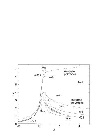
Figure 15: Generalized caloric curve for $2<D<4$ (specifically $D=3$). For $n_{3}<n<n_{5}$, the inverse temperature presents a maximum but not the energy. For $n>n_{3}$, there exists a region of negative (generalized) specific heats $C=dE/dT<0$ in the microcanonical ensemble. We have plotted in dashed line the branch of complete polytropes with $R_{*}<R$ defined by Eq. (109).

Figure 16: Generalized caloric curve for $4<D<10$ (specifically $D=4.5$). For $n<n_{3}$ (specifically $n_{3}=1.8$), the energy presents a minimum but not the inverse temperature. For $n_{3}<n<n_{3/2}$ (specifically $n_{3/2}=2.25$), both the energy and the temperature present a minimum and the caloric curve $\eta(\Lambda)$ rotates anti-clockwise. This implies that equilibrium states with positive as well as negative specific heats $C=dE/dT$ are stable in the canonical ensemble. This “thermodynamical anomaly” arises because, as discussed in Sec. 3.1, stellar polytropes with $n<n_{3/2}$ are unphysical (the temperature is negative). For $n=n_{3/2}$ (white dwarfs), the curve makes an angular point (see Appendix C).

Figure 17: Continuation of Fig. 16. For $n_{3/2}<n<n_{5}$ (specifically $n_{5}=2.6$) both the energy and the temperature present an extremum and the curve rotates clockwise (the curve makes a “loop”). The region of negative specific heats is now unstable in the canonical ensemble, as it should. For $n>n_{5}$ (specifically $n_{5}=2.6$), the energy and temperature present an infinity of extrema.

Figure 18: Generalized caloric curve for $D>2(1+\sqrt{2})$ (specifically $D=5.1$) and $n=n_{3/2}$. For this particular index, the curve presents an infinity (because $n_{3/2}>n_{5}$) of angular points towards the singular sphere (see Appendix C).

Figure 19: This figure summarizes the structure of the caloric curve as a function of the dimension $D$ and the polytropic index $n$. The symbols are defined in the text. If we limit ourselves to $n\geq D/2$ (physical stellar polytropes), the region $AB^{\prime}$ showing a “thermodynamical anomaly” is not accessible.

The curve $\Lambda(\alpha)$ presents an extremum at points $\alpha^{\prime}_{k}$ such that $d\Lambda/d\alpha(\alpha^{\prime}_{k})=0$. Using Eqs. (102), (71) and (72), we find that this condition is equivalent to

$$2(n+1-D)u_{0}^{2}+(n+1)(n+1-D)u_{0}v_{0}+2(D-n-1)(D-1)u_{0}$$

(117) $$+{1\over 2}D(D-4)(n+1)u_{0}+{1\over 2}D(D-4)(n+1)v_{0}+{1\over 2}D(D-4)(2-D)(n+1)=0.$$

We can check that the point $(u_{s},v_{s})$ is a solution of this equation. On the other hand, $v_{0}=D-2$ for $u_{0}=0$ and $v_{0}\sim-2u_{0}/(n+1)$ for $u_{0}\rightarrow\pm\infty$. Finally, $v_{0}\rightarrow\infty$ for $u_{0}\rightarrow u_{*}$ where

(118) $$u_{*}={D(4-D)\over 2(n+1-D)}.$$

More precisely, for $u_{0}\rightarrow u_{*}$, we have

(119) $$(u_{0}-u_{*})v_{0}\sim{D(D-4)(D-2)\over 2(n+1)(D-n-1)^{2}}(n-n_{3/2})(n-n_{5})\equiv\Delta_{2}(n).$$

The two roots of $\Delta_{2}(n)$ are $n=n_{3/2}$ and $n=n_{5}$. They coincide at the particular dimension $D=2(1+\sqrt{2})$. We note also that $u_{*}=0$ for $D=4$. For $D>2$ and $n=D-1$, Eq. (117) reduces to $u+v=D-2$.

The points where $\Lambda(\alpha)$ is extremum are determined by the intersections between the solution curve in the $(u,v)$ plane and the curve defined by Eq. (117). The number of extrema can thus be determined by a graphical construction using Figs. 1-4. This graphical construction depends on the values of $D$ and $n$ and the different cases are shown in Figs. 7-10. For $D<2$, there is no extremum (case $A^{\prime}$). For $2<D<4$, there is no extremum for $n<n_{5}$ (case $A^{\prime}$) and there is an infinity of extrema for $n>n_{5}$ (case $C^{\prime}$). They exhibit damped oscillations toward the value $\Lambda_{s}$ corresponding to the singular solution (47). For $4<D<10$, there is one maximum for $n<n_{5}$ (case $B^{\prime}$) and there is an infinity of extrema for $n>n_{5}$ (case $C^{\prime}$). For $D>10$, there is one maximum for $n<n_{5}$ (case $B^{\prime}$), there is an infinity of extrema for $n_{5}<n<n_{-}$ (case $C^{\prime}$), and there is no extremum for $n>n_{-}$ (case $D^{\prime}$). This last case corresponds to an overdamped evolution towards the value $\Lambda_{s}$ (in our mechanical analogy of Sec. 3.3). The appearance of a maximum for $n<n_{5}$ when $D>4$ was a surprise in view of preceding analysis for $D=3$ [27, 29, 26]. The parameter $\Lambda$ is restricted by the inequalities (see Figs. 11 and 12)

(120) $$\Lambda\leq\lambda_{n}\qquad({\rm case\ A^{\prime}}),$$

(121) $$\Lambda<\Lambda(\alpha_{1})\qquad({\rm cases\ B^{\prime}\ and\ C^{\prime}}),$$

(122) $$\Lambda\leq\Lambda_{s}\qquad({\rm case\ D^{\prime}}).$$

These inequalities determine a minimum energy (for given $M$ and $R$) below which the system will either converge toward a complete polytrope with radius $R_{*}<R$ (if it is stable) or collapse.

In Figs. 13-18, we have plotted the generalized caloric curve $\Lambda-\eta$, giving the inverse temperature as a function of the energy, for different dimensions $D$ and polytropic index $n$. This extends the results of our previous analysis in $D=3$ [29]. The number of turning points as a function of $D$ and $n$ is recapitulated in Fig. 19.

3.7 The generalized thermodynamical stability

We now come to the generalized thermodynamical stability problem. We shall say that a polytrope is stable if it corresponds to a maximum of Tsallis entropy (free energy) at fixed mass and energy (temperature) in the microcanonical (canonical) ensemble. The stability analysis has already been performed for $D=3$ [27, 29, 28, 26] and is extended here to a space of arbitrary dimension. This stability analysis can be used to settle either (i) the dynamical stability of stellar and gaseous polytropes (see Sec. 2) or (ii) the generalized thermodynamical stability of self-gravitating Langevin particles (see Sec. 4).

We start by the canonical ensemble which is simpler in a first approach. A polytropic distribution is a local minimum of free energy at fixed mass and temperature if, and only if, the second order variations (see Appendix D)

(123) $$\delta^{2}F={n+1\over 2n}\int{p\over\rho^{2}}(\delta\rho)^{2}d^{D}{\bf r}+{1\over 2}\int\delta\rho\delta\Phi d^{D}{\bf r},$$

are positive for any perturbation $\delta\rho$ that conserves mass, i.e.

(124) $$\int\delta\rho\ d^{D}{\bf r}=0.$$

This is the condition of (generalized) thermodynamical stability in the canonical ensemble. Introducing the function $q(r)$ by the relation

(125) $$\delta\rho={1\over S_{D}r^{D-1}}{dq\over dr},$$

and integrating by parts, we can put the second order variations of free energy in the quadratic form

(126) $$\delta^{2}F=-{1\over 2}\int_{0}^{R}drq\biggl{[}K\gamma{d\over dr}\biggl{(}{\rho^{\gamma-2}\over S_{D}r^{D-1}}{d\over dr}\biggr{)}+{G\over r^{D-1}}\biggr{]}q.$$

The second order variations of free energy can be negative (implying instability) only if the differential operator which occurs in the integral has positive eigenvalues. We need therefore to consider the eigenvalue problem

(127) $$\biggl{[}K\gamma{d\over dr}\biggl{(}{\rho^{\gamma-2}\over S_{D}r^{D-1}}{d\over dr}\biggr{)}+{G\over r^{D-1}}\biggr{]}q_{\lambda}(r)=\lambda q_{\lambda}(r).$$

with $q_{\lambda}(0)=q_{\lambda}(R)=0$ in order to satisfy the conservation of mass. If all the eigenvalues $\lambda$ are negative, the polytrope is a minimum of free energy. If at least one eigenvalue is positive, the polytrope is an unstable saddle point. The point of marginal stability in the series of equilibria is determined by the condition that the largest eigenvalue is equal to zero ($\lambda=0$). We thus have to solve the differential equation

(128) $$K\gamma{d\over dr}\biggl{(}{\rho^{\gamma-2}\over S_{D}r^{D-1}}{dF\over dr}\biggr{)}+{GF\over r^{D-1}}=0,$$

with $F(0)=F(R)=0$. The same eigenvalue equation is obtained by studying the linear stability of the Euler-Jeans equation [29, 26]. Introducing the dimensionless variables defined previously, we can rewrite this equation in the form

(129) $${d\over d\xi}\biggl{(}{\theta^{1-n}\over\xi^{D-1}}{dF\over d\xi}\biggr{)}+{nF\over\xi^{D-1}}=0,$$

with $F(0)=F(\alpha)=0$. If

(130) $${\cal L}\equiv{d\over d\xi}\biggl{(}{\theta^{1-n}\over\xi^{D-1}}{d\over d\xi}\biggr{)}+{n\over\xi^{D-1}}$$

denotes the differential operator occurring in Eq. (129), we can check by using the Emden Eq. (45) that

(131) $${\cal L}(\xi^{D-1}\theta^{\prime})=(n-1)\theta^{\prime},\qquad{\cal L}(\xi^{D}\theta^{n})=[(2-D)n+D]\theta^{\prime}.$$

Therefore, the general solution of Eq. (129) satisfying the boundary conditions at $\xi=0$ is

(132) $$F(\xi)=c_{1}\biggl{[}\xi^{D}\theta^{n}+{(D-2)n-D\over n-1}\xi^{D-1}\theta^{\prime}\biggr{]}.$$

Using Eq. (132) and introducing the Milne variables (70), the condition $F(\alpha)=0$ can be written

(133) $$u_{0}={(D-2)n-D\over n-1}=u_{s}.$$

This relation determines the points at which a new eigenvalue becomes positive ($\lambda=0^{+}$). Comparing with Eq. (113), we see that a mode of stability is lost each time that $\eta$ is extremum in the series of equilibria, in agreement with the turning point criterion of Katz [41] in the canonical ensemble. When the curve $\eta(\alpha)$ is monotonic (cases $A$ and $D$), the system is always stable because it is stable at low density contrasts $(\alpha\rightarrow 0)$ and no change of stability occurs afterward. When the curve $\eta(\alpha)$ presents extrema (cases $B$ and $C$), the series of equilibria becomes unstable at the point of minimum temperature (or maximum mass) $\alpha_{1}$. In Fig. 15, this corresponds to a point of infinite specific heat $C=dE/dT\rightarrow\infty$, just before entering the region of negative specific heats $C<0$. When the curve $\eta(\alpha)$ presents several extrema (case $C$), secondary modes of instability appear at values $\alpha_{2}$, $\alpha_{3}$,… (see [29] in $D=3$). We note that complete polytropes (with $n<n_{5}$ if $D>2$) are stable in the canonical ensemble if $D\leq 2$ and if ($D>2$, $n\leq n_{3}$). They are unstable otherwise. In the thermodynamical analogy developed in [29, 26], this is a condition of nonlinear dynamical stability for gaseous polytropes with respect to the Jeans-Euler equations. In particular, the self-gravitating Fermi gas at zero temperature (a classical white dwarf star) is dynamically stable if $n_{3/2}<n_{3}$, i.e. $D<4$, and unstable otherwise.

Figure 20: Location of the turning points of temperature in the $(u,v)$ plane for systems with dimension $2<D<10$ (specifically $D=3$). The line $u=u_{s}$ determines the extrema of $\eta$ and the line $v=v_{s}$ determines the nodes of the density profiles that trigger the instabilities in the canonical ensemble.

According to Eq. (125), the perturbation profile that triggers a mode of instability at the critical point $\lambda=0$ is given by

(134) $${\delta\rho\over\rho_{0}}={1\over S_{D}\xi^{D-1}}{dF\over d\xi},$$

where $F(\xi)$ is given by Eq. (132). Introducing the Milne variables (70), we get

(135) $${\delta\rho\over\rho}={nc_{1}\over S_{D}}(v_{s}-v).$$

The density perturbation $\delta\rho$ becomes zero at point(s) $\xi_{i}$ such that $v(\xi_{i})=v_{s}$. The number of nodes is therefore given by the number of intersections between the solution curve in the $(u,v)$ plane and the line $v=v_{s}$. It can be determined by straightforward graphical constructions in the Milne plane, using Figs. 1-4 (see, e.g., Fig. 20). When the solution curve is monotonic (case $B$), the density perturbation profile has only one node. In particular, for $n=n_{5}$, the perturbation profile at the point of marginal stability is given by

(136) $${\delta\rho\over\rho}={(D+2)c_{1}\over 2S_{D}}{D(D-2)-\xi^{2}\over D(D-2)+\xi^{2}}.$$

It vanishes for $\xi_{(1)}=\sqrt{D(D-2)}$. When the solution curve forms a spiral (case $C$), the density perturbation $\delta\rho$ corresponding to the $k$-th mode of instability has $k$ zeros $\xi_{1},\xi_{2},...,\xi_{k}<\alpha_{k}$. In particular, the first mode of instability has only one node. For high modes of instability, the zeros asymptotically follow a geometric progression with ratio $1:{\rm exp}\{2\pi/\sqrt{-\Delta}\}$ (see Ref. [29] for $D=3$).

In the microcanonical ensemble, a polytrope is a maximum of entropy at fixed mass and energy if, and only if, the second order variations (see Appendix D)

$${\delta^{2}S}=\beta\Biggl{\{}-{1\over 2}\gamma\int p{(\delta\rho)^{2}\over\rho^{2}}d^{D}{\bf r}-{1\over 2}\int\delta\rho\delta\Phi d^{D}{\bf r}$$

(137) $$-{2n\over D(2n-D)}{1\over\int pd^{D}{\bf r}}\biggl{[}\int\biggl{(}\Phi+{D\over 2}\gamma{p\over\rho}\biggr{)}\delta\rho d^{D}{\bf r}\biggr{]}^{2}\Biggr{\}},$$

are negative for any variation $\delta\rho$ that conserves mass to first order (the conservation of energy has already been taken into account in obtaining Eq. (137)). Now, using Eq. (125) and integrating by parts, the second variations of entropy can be put in a quadratic form

(138) $$\delta^{2}S=\int_{0}^{R}\int_{0}^{R}drdr^{\prime}q(r)K(r,r^{\prime})q(r^{\prime}),$$

with

$$K(r,r^{\prime})=-{2n\over D(2n-D)}{1\over\int pd^{D}{\bf r}}\biggl{(}\Phi+{D\over 2}K\gamma\rho^{\gamma-1}\biggr{)}^{\prime}(r)\biggl{(}\Phi+{D\over 2}K\gamma\rho^{\gamma-1}\biggr{)}^{\prime}(r^{\prime})$$

(139) $$+{1\over 2}\delta(r-r^{\prime})\biggl{[}K\gamma{d\over dr}\biggl{(}{\rho^{\gamma-2}\over S_{D}r^{D-1}}{d\over dr}\biggr{)}+{G\over r^{D-1}}\biggr{]}.$$

The problem of stability can therefore be reduced to the study of the eigenvalue equation

(140) $$\int_{0}^{R}dr^{\prime}K(r,r^{\prime})q_{\lambda}(r^{\prime})=\lambda q_{\lambda}(r),$$

with $q_{\lambda}(0)=q_{\lambda}(R)=0$. The point of marginal stability ($\lambda=0$) will be determined by solving the differential equation

(141) $$K\gamma{d\over dr}\biggl{(}{\rho^{\gamma-2}\over S_{D}r^{D-1}}{dF\over dr}\biggr{)}+{GF\over r^{D-1}}={K\gamma^{2}\over DnS_{D}}(2n-D)V\rho^{\gamma-2}{d\rho\over dr},$$

with

(142) $$V={\int_{0}^{R}\rho^{\gamma-2}{d\rho\over dr}Fdr\over\int_{0}^{R}\rho^{\gamma}r^{D-1}dr}.$$

In arriving at this expression, we have used the relation

(143) $$\biggl{(}\Phi+{D\over 2}K\gamma\rho^{\gamma-1}\biggr{)}^{\prime}={K\gamma\over 2n}(D-2n)\rho^{\gamma-2}{d\rho\over dr},$$

which results from the condition of hydrostatic equilibrium (13) with the polytropic equation of state (30). Introducing the dimensionless variables defined previously, Eqs. (141) and (142) can be rewritten

(144) $${d\over d\xi}\biggl{(}{\theta^{1-n}\over\xi^{D-1}}{dF\over d\xi}\biggr{)}+{nF\over\xi^{D-1}}=\chi\theta^{\prime},$$

with

(145) $$\chi={1\over D}(n+1)(2n-D){\int_{0}^{\alpha}\theta^{\prime}Fd\xi\over\int_{0}^{\alpha}\theta^{n+1}\xi^{D-1}d\xi},$$

and $F(0)=F(\alpha)=0$. Using the identities (131), we can check that the general solution of Eq. (144) satisfying the boundary conditions for $\xi=0$ and $\xi=\alpha$ is

(146) $$F(\xi)={\chi\over(n-1)u_{0}+D-(D-2)n}(\xi^{D}\theta^{n}+u_{0}\xi^{D-1}\theta^{\prime}).$$

The point of marginal stability is then obtained by substituting the solution (146) in Eq. (145). Using the identities (see Appendix E)

(147) $$\int_{0}^{\alpha}\xi^{D-1}(\theta^{\prime})^{2}d\xi={\alpha^{D}\theta^{\prime}(\alpha)^{2}\over D+2-(D-2)n}\biggl{(}n+1+2{u_{0}\over v_{0}}-{2D\over v_{0}}\biggr{)},$$

(148) $$\int_{0}^{\alpha}\theta^{n+1}\xi^{D-1}d\xi={\alpha^{D}\theta^{\prime}(\alpha)^{2}\over D+2-(D-2)n}\biggl{(}n+1+2{u_{0}\over v_{0}}-{(D-2)(n+1)\over v_{0}}\biggr{)},$$

(149) $$\int_{0}^{\alpha}\theta^{n}\theta^{\prime}\xi^{D}d\xi={\alpha^{D}\theta^{\prime}(\alpha)^{2}\over D+2-(D-2)n}\biggl{(}-D-(D-2){u_{0}\over v_{0}}+{D(D-2)\over v_{0}}\biggr{)},$$

which result from simple integrations by parts and from the properties of the Lane-Emden equation (45), it is found that the point of marginal stability is determined by the condition (117). Therefore, the series of equilibria becomes unstable at the point of minimum energy in agreement with the turning point criterion of Katz [41] in the microcanonical ensemble. When the curve $\Lambda(\alpha)$ is monotonic (cases $A^{\prime}$ and $D^{\prime}$), the system is always stable. When the curve $\Lambda(\alpha)$ presents extrema (cases $B^{\prime}$ and $C^{\prime}$), the series of equilibria becomes unstable at the point of minimum energy $\alpha^{\prime}_{1}$. In Fig. 15, this corresponds to the point where the specific heat $C=dE/dT=0$, passing from negative to positive values. Note that the branch of negative specific heats between $CE$ and $MCE$ is stable in the microcanonical ensemble although it is unstable in the canonical ensemble. When the curve $\Lambda(\alpha)$ presents several extrema (case $C^{\prime}$), secondary modes of instability appear at values $\alpha^{\prime}_{2}$, $\alpha^{\prime}_{3}$,… We note that complete polytropes (with $n<n_{5}$ if $D>2$) are stable in the microcanonical ensemble if $D<4$ and unstable if $D\geq 4$. Owing to the thermodynamical analogy, this is a condition of nonlinear dynamical stability for stellar polytropes with respect to the Vlasov equation [26]. The difference between the dynamical stability of gaseous polytropes ($n\leq n_{3}$) and stellar polytropes ($n\leq n_{5}$) was related in [29, 26] to a situation of ensemble inequivalence (and the existence of a negative specific heat region) in thermodynamics. Since the caloric curve is monotonic in $D=2$, we also conclude that polytropic vortices [20] are always nonlinearly dynamically stable with respect to the 2D Euler equation.

According to Eqs. (134) and (146), the perturbation profile that triggers a mode of instability at the critical point $\lambda=0$ is given by

(150) $${\delta\rho\over\rho}={\chi\over S_{D}}{1\over(n-1)u_{0}+D-(D-2)n}(D-nv-u_{0}),$$

where we have used the Emden equation (45) and introduced the Milne variables (70). The number of nodes in the perturbation profile can be determined by a graphical construction similar to the one described in Refs. [42, 3] for $n=\infty$ (isothermal case).

4 Self-gravitating Langevin particles

4.1 The nonlinear Smoluchowski-Poisson system

Let us consider a system of $N$ self-gravitating Brownian particles described by the stochastic equations ($i=1,...,N$)

(151) $${d{\bf r}_{i}\over dt}={\bf v}_{i},\qquad{d{\bf v}_{i}\over dt}=-\nabla\Phi_{i}-\xi{\bf v}_{i}+\sqrt{2T\xi}\ {\bf R}_{i}(t),$$

where $\Phi_{i}=\Phi({\bf r}_{i},t)$ is the self-consistent gravitational potential created by the particles, $-\xi{\bf v}_{i}$ is a friction force originating from the presence of an inert medium and ${\bf R}_{i}(t)$ is a white noise satisfying $\langle{\bf R}_{i}(t)\rangle=0$ and $\langle{R}_{i,a}(t){R}_{j,b}(t^{\prime})\rangle=\delta_{ij}\delta_{ab}\delta(t-t^{\prime})$. To simplify the problem, we consider the high friction limit $\xi\rightarrow+\infty$, where $\xi$ is the friction coefficient [2]. This regime is achieved for times $t\gg\xi^{-1}$. In the mean-field approximation, the evolution of the density of particles is governed by the Smoluchowski equation [10]

(152) $${\partial\rho\over\partial t}=\nabla\biggl{[}\nabla(D\rho)+{1\over\xi}\rho\nabla\Phi\biggr{]},$$

coupled to the Newton-Poisson equation (4). In the usual case [2, 3, 4], the diffusion coefficient $D$ is constant and the condition that the Boltzmann distribution $\rho\sim{\rm e}^{-\Phi/T}$ is a stationary solution of Eq. (152) is ensured by the Einstein relation $\xi D=T$. It can be shown [2] that the SP system decreases the free energy $F=E-TS$ constructed with the Boltzmann entropy. Hence, the equilibrium state minimizes

(153) $$F={1\over 2}\int\rho\Phi d^{D}{\bf r}+T\int\rho\ln\rho d^{D}{\bf r},$$

at fixed $M$ and $T$.

We want to consider here a more general situation in which the diffusion coefficient $D$ depends on the density $\rho$ while the drift coefficient $\xi$ is still constant. In the absence of drift, this would lead to a situation of anomalous diffusion. In the presence of drift, a notion of generalized thermodynamics emerges [20]. Indeed, writing the diffusion coefficient in the form $D(\rho)={1\over\xi}p(\rho)/\rho$, we obtain the generalized Smoluchowski equation

(154) $${\partial\rho\over\partial t}=\nabla\biggl{[}{1\over\xi}(\nabla p+\rho\nabla\Phi)\biggr{]}.$$

In Ref. [20], it is shown that generalized Smoluchowski equations of this type satisfy a form of canonical $H$-theorem. The Lyapunov functional decreasing monotonically with time is

(155) $$F=\int\rho\int_{0}^{\rho}{p(\rho^{\prime})\over\rho^{{}^{\prime}2}}d\rho^{\prime}d^{D}{\bf r}+{1\over 2}\int\rho\Phi d^{D}{\bf r}.$$

This can be interpreted as a free energy associated with a generalized entropy functional (see [20] for more details). The equilibrium state minimizes $F$ at fixed $M$. In the present context, this is a condition of generalized thermodynamical stability in canonical ensemble.

The generalized Smoluchowski equation (154) can be obtained by combining the ordinary Fokker-Planck equation with a Langevin equation of the form [20]:

(156) $${d{\bf r}\over dt}=-{1\over\xi}\nabla\Phi+\sqrt{2p(\rho)\over\xi\rho}{\bf R}(t),$$

where ${\bf R}(t)$ is a white noise. When $p(\rho)$ is a power-law, Eq. (156) reduces to the stochastic equations studied by Borland [21] in connexion with Tsallis thermodynamics. Since the function in front of ${\bf R}(t)$ depends on ${\bf r}$, the last term in Eq. (156) can be interpreted as a multiplicative noise. Note that the noise depends on ${\bf r}$ through the density $\rho({\bf r})$. Kaniadakis [22] has also introduced generalized Fokker-Planck equation arising from a modified form of transition probabilities. In these works, the Langevin particles evolve in an external potential. The case of Langevin particles in interaction was considered by Chavanis [20]. He introduced a generalized Fokker-Planck equation (see in particular Eq. (81) of [20]) valid for an arbitrary equation of state $p=p(\rho)$, or diffusion coefficient $D(\rho)$, and for an arbitrary binary potential of interaction $u({\bf r}-{\bf r}^{\prime})$. This equation has been studied recently in [1, 2, 3, 4] for an isothermal equation of state $p=\rho T$ (constant $D$) and a gravitational interaction. This study has been extended in [43] to a Fermi-Dirac equation of state. In this paper, we consider the case where the function $D(\rho)$ is a power law and write $\xi D(\rho)=K\rho^{\gamma-1}$. This corresponds to a polytropic equation of state $p=K\rho^{\gamma}$. Then, Eq. (152) can be rewritten

(157) $${\partial\rho\over\partial t}=\nabla\biggl{[}{1\over\xi}(K\nabla\rho^{\gamma}+\rho\nabla\Phi)\biggr{]}.$$

For the nonlinear Smoluchowski-Poisson system, the Lyapunov functional decreasing monotonically with time is [20]

(158) $$F={K\over\gamma-1}\int(\rho^{\gamma}-\rho)d^{D}{\bf r}+{1\over 2}\int\rho\Phi d^{D}{\bf r}.$$

It can be interpreted as a free energy associated with Tsallis entropy. In this context, the polytropic index $\gamma$ plays the role of the $q$-parameter and the polytropic constant $K$ plays the role of the temperature (see Ref. [20] for details and subtleties). Therefore, keeping $K$ fixed corresponds to a canonical situation [29]. For $\gamma\rightarrow 1$, we recover the Boltzmann free energy studied in [2, 3]. For $\gamma=5/3$, i.e. $n=3/2$, Eq. (157) describes self-gravitating Brownian fermions at $T=0$ (in $D=3$) [43].

The nonlinear Smoluchowski equation can be obtained from a variational principle, called Maximum Entropy Production Principle, by maximizing the rate of free energy $\dot{F}$ for a fixed total mass $M$ [1, 20]. It is straightforward to check that the rate of free energy dissipation can be put in the form

(159) $$\dot{F}=-\int{1\over\rho\xi}(K\nabla\rho^{\gamma}+\rho\nabla\Phi)^{2}d^{D}{\bf r}\leq 0.$$

For a stationary solution, $\dot{F}=0$, and we obtain a polytropic distribution which is a critical point of $F$ at fixed $M$. Considering a small perturbation around equilibrium, we can establish the identity [20]:

(160) $$\delta^{2}\dot{F}=2\lambda\delta^{2}F\leq 0,$$

where $\lambda$ is the growth rate of the perturbation defined such that $\delta\rho\sim{\rm e}^{\lambda t}$. This relation shows that a stationary solution of the nonlinear Smoluchowski-Poisson (NSP) system is dynamically stable for small perturbations ($\lambda<0$) if and only if it is a local minimum of free energy ($\delta^{2}F>0$). In addition, it is shown in Refs. [2, 20] that the eigenvalue problem determining the growth rate $\lambda$ of the perturbation is similar to the eigenvalue problem (128) associated with the second order variations of free energy (they coincide for marginal stability). This shows the equivalence between dynamical and generalized thermodynamical stability for self-gravitating Langevin particles exhibiting anomalous diffusion (this result was obtained independently by Shiino [24] in the specific context of Tsallis thermodynamics). In fact, our formalism is valid for more general functionals than the Boltzmann or the Tsallis entropies [20]. These functionals (155) arise when the diffusion coefficient is of the general form $D(\rho)$, not necessarily a power law. We note that the NSP system satisfies a form of Virial theorem [20]. For $D\neq 2$, it reads

(161) $${1\over 2}\xi{dI\over dt}=2K+(D-2)W-Dp_{b}V,$$

where

(162) $$I=\int\rho r^{2}d^{D}{\bf r},$$

is the moment of inertia and $p_{b}$ the pressure on the box (assumed uniform). For $D=2$, the term $(D-2)W$ is replaced by $-GM^{2}/2$. For a stationary solution $dI/dt=0$, we recover the Virial theorem (91).

Our model of self-gravitating Brownian (or Langevin) particles has no clear astrophysical applications, so it must be regarded essentially as a toy model of gravitational dynamics. It may find application for the formation of planetesimals in the solar nebula since the dust particles experience a friction with the gas and a noise due to small-scale turbulence [44]. However, even in this context, the model has to be refined so as to take into account the attraction of the Sun and the rotation of the disk. Anyway, the self-gravitating Brownian (or Langevin) gas model is well-posed mathematically, and it possesses a rigorous thermodynamical structure corresponding to the canonical ensemble. Therefore, it can be used as a simple model to illustrate some aspects of the thermodynamics of self-gravitating systems. Since it minimizes $F={\cal W}[\rho]$ at fixed mass, it can also be used as a powerful numerical algorithm to construct nonlinearly dynamically stable stationary solutions of the Euler-Jeans equations (see Sec. 2.2). Coincidentally, the SP system also provides a simple model for the chemotactic aggregation of bacterial populations [11]. The name chemotaxis refers to the motion of organisms induced by chemical signals. In some cases, the biological organisms secrete a substance that has an attractive effect on the organisms themselves. This is the case for the bacteria Escherichia coli. In the simplest model, the bacteria have a diffusive motion and they also move systematically along the gradient of concentration of the chemical they secrete. Since the density $\Phi({\bf r},t)$ of the secreted substance is induced by the particles themselves, the drift is directed toward the region of higher density. This attraction triggers a self-accelerating process until a point at which aggregation takes place. If we assume in a first step that $\Phi({\bf r},t)$ is related to the bacterial density $\rho({\bf r},t)$ by a Poisson equation, this phenomenon can be modeled by the SP system. Now, it has been observed in many occasions in biology that the diffusion of the particles is anomalous [11]. This is a physical motivation to study the NSP system in which the diffusion coefficient is a power law of the density. In the following section, we show that the NSP system admits self-similar solutions describing the collapse of the self-gravitating Langevin gas or of the bacterial population. These theoretical results are confirmed in Sec. 5 where we numerically solve the NSP system.

4.2 Self-similar solutions of the nonlinear Smoluchowski-Poisson system

From now on, we set $M=R=G=\xi=1$ without loss of generality. The equations of the problem become

(163) $${\partial\rho\over\partial t}=\nabla(K\nabla\rho^{\gamma}+\rho\nabla\Phi),$$

(164) $$\Delta\Phi=S_{D}\rho,$$

with boundary conditions

(165) $${\partial\Phi\over\partial r}(0,t)=0,\qquad\Phi(1)={1\over 2-D},\qquad K{\partial\rho^{\gamma}\over\partial r}(1)+\rho(1)=0,$$

for $D\neq 2$. For $D=2$, we take $\Phi(1)=0$ on the boundary. We restrict ourselves to spherically symmetric solutions. Integrating Eq. (164) once, we can rewrite the NSP system in the form of a single integrodifferential equation

(166) $${\partial\rho\over\partial t}={1\over r^{D-1}}{\partial\over\partial r}\biggl{\{}r^{D-1}\biggl{[}(S_{D}\rho)^{1/n}\Theta{\partial\rho\over\partial r}+{\rho\over r^{D-1}}\int_{0}^{r}\rho(r^{\prime})S_{D}r^{{}^{\prime}D-1}dr^{\prime}\biggr{]}\biggr{\}},$$

where we have set

(167) $$\Theta\equiv{K(1+n)\over nS_{D}^{1/n}}={1\over n\eta^{1-1/n}}.$$

The quantity $\Theta$ can be seen as a sort of generalized temperature (sometimes called a polytropic temperature [29]) and it reduces to the ordinary temperature $T$ for $n\rightarrow+\infty$. We note that the proper description of a gas of Langevin particles in interactions is the canonical ensemble where $\Theta$ is fixed. However, we can formally set up a microcanonical description of self-gravitating Langevin particles by letting the temperature $\Theta(t)$ depend on time so as to conserve the total energy:

(168) $$E={D\over 2}{nS_{D}^{1/n}\over 1+n}\int\Theta(t)\rho^{1+{1\over n}}d^{D}{\bf r}+{1\over 2}\int\rho\Phi d^{D}{\bf r}.$$

The two situations have been considered in the case of self-gravitating Brownian particles ($n\rightarrow+\infty$) in [1, 2, 3, 4].

The NSP system is also equivalent to a single differential equation

(169) $$\frac{\partial M}{\partial t}=\Theta\biggl{(}{1\over r^{D-1}}{\partial M\over\partial r}\biggr{)}^{1/n}\biggl{[}{\partial^{2}M\over\partial r^{2}}-{D-1\over r}{\partial M\over\partial r}\biggr{]}+{M\over r^{D-1}}{\partial M\over\partial r},$$

for the quantity

(170) $$M(r,t)=\int_{0}^{r}\rho(r^{\prime},t)S_{D}r^{{}^{\prime}D-1}dr^{\prime},$$

which represents the mass contained within the sphere of radius $r$. The appropriate boundary conditions are

(171) $$M(0,t)=0,\qquad M(1,t)=1.$$

It is also convenient to introduce the function $s(r,t)=M(r,t)/r^{D}$ satisfying

(172) $${\partial s\over\partial t}=\Theta\biggl{(}r{\partial s\over\partial r}+Ds\biggr{)}^{1/n}\biggl{(}{\partial^{2}s\over\partial r^{2}}+{D+1\over r}{\partial s\over\partial r}\biggr{)}+\biggl{(}r{\partial s\over\partial r}+Ds\biggr{)}s.$$

For $n\rightarrow+\infty$, these equations reduce to those studied in Refs. [2, 3, 4] in the isothermal case. We look for self-similar solutions of the form

(173) $$\rho(r,t)=\rho_{0}(t)f\biggl{(}{r\over r_{0}(t)}\biggr{)},\qquad r_{0}=\biggl{(}{\Theta\over\rho_{0}^{1-1/n}}\biggr{)}^{1/2}.$$

The radius $r_{0}$ defined by the foregoing equation provides a typical value of the core radius of an incomplete polytrope (with $n>n_{5}$). It reduces to the King’s radius [19] as $n\rightarrow+\infty$. In terms of the mass profile, we have

(174) $$M(r,t)=M_{0}(t)g\biggl{(}{r\over r_{0}(t)}\biggr{)},\qquad{\rm with}\qquad M_{0}(t)=\rho_{0}r_{0}^{D},$$

and

(175) $$g(x)=\int_{0}^{x}f(x^{\prime})S_{D}x^{{}^{\prime}D-1}dx^{\prime}.$$

In terms of the function $s$, we have

(176) $$s(r,t)=\rho_{0}(t)S\biggl{(}{r\over r_{0}(t)}\biggr{)},\qquad{\rm with}\qquad S(x)={g(x)\over x^{D}}.$$

Substituting the ansatz (176) into Eq. (172), and using the definition of $r_{0}$ in Eq. (173), we find that

(177) $${d\rho_{0}\over dt}S-{\rho_{0}\over r_{0}}{dr_{0}\over dt}xS^{\prime}=\rho_{0}^{2}(xS^{\prime}+DS)^{1/n}\biggl{(}S^{\prime\prime}+{D+1\over x}S^{\prime}\biggr{)}+\rho_{0}^{2}(xS^{\prime}+DS)S,$$

where we have set $x=r/r_{0}$. We now assume that there exists $\alpha$ such that

(178) $$\rho_{0}\sim r_{0}^{-\alpha}.$$

Inserting this relation into Eq. (177), we find

(179) $${d\rho_{0}\over dt}\biggl{(}S+{1\over\alpha}xS^{\prime}\biggr{)}=\rho_{0}^{2}\biggl{[}(xS^{\prime}+DS)^{1/n}\biggl{(}S^{\prime\prime}+{D+1\over x}S^{\prime}\biggr{)}+(xS^{\prime}+DS)S\biggr{]},$$

which implies that $(1/\rho_{0}^{2})(d\rho_{0}/dt)$ is a constant that we arbitrarily set equal to $\alpha$. This leads to

(180) $$\rho_{0}(t)={1\over\alpha}(t_{coll}-t)^{-1},$$

so that the central density becomes infinite in a finite time $t_{coll}$. The scaling equation now reads

(181) $$\alpha S+xS^{\prime}=(xS^{\prime}+DS)^{1/n}\biggl{(}S^{\prime\prime}+{D+1\over x}S^{\prime}\biggr{)}+(xS^{\prime}+DS)S.$$

For $x\rightarrow+\infty$, we have asymptotically

(182) $$S(x)\sim x^{-\alpha},\qquad g(x)\sim x^{D-\alpha},\qquad f(x)\sim x^{-\alpha}.$$

In the canonical ensemble where $\Theta$ is constant, Eq. (173) and Eq. (178) lead to $\alpha=\alpha_{n}$, with

(183) $$\alpha_{n}=\frac{2n}{n-1}.$$

Note that for $n\to\infty$, we recover the result of [3], $\alpha_{\infty}=2$. Equation (182) implies that for large $x$, $\rho\sim(D-\alpha)S>0$, which enforces $\alpha<D$ (this also guarantees that the mass of the power-law profile $\rho=Cr^{-\alpha}$ at $t=t_{coll}$ is finite). The limit value $\alpha_{n}=D$ corresponds to $n=n_{3}$. Therefore, there is no scaling solution for $n<n_{3}$. This is consistent with our finding that the collapse occurs only for $n>n_{3}$. For $n<n_{3}$ and $\eta>\omega_{n}$, the system converges toward a complete polytrope with radius $R_{*}<1$ which is stable (see Sec. 3.7 and Fig. 15). For $n_{3}<n<n_{5}$ and $\eta>\eta(\alpha_{1})$, we can formally construct a complete polytrope with radius $R_{*}<1$, but this structure is unstable (Sec. 3.7) so that the system undergoes gravitational collapse.

In the microcanonical ensemble, the value of $\alpha\geq\alpha_{n}$ cannot be obtained by dimensional analysis. It will be selected by the dynamics. In the case $n\to+\infty$, we have found in [3] that Eq. (181) for the scaling profile has physical solutions only for $2\leq\alpha\leq\alpha_{\rm max}(D)$ (with $\alpha_{\rm max}(D=3)=2.209733...$). For arbitrary $n$, such a $\alpha_{\rm max}(D,n)\geq\alpha_{n}$ also exists (see Sec. 5). It is easy to see that the maximum value for $\alpha$ leads to the maximum divergence of temperature and entropy. Therefore, it is natural to expect that the value $\alpha_{\rm max}$ will be selected by the dynamics except if some kinetic constraints forbid this natural evolution (see below). In fact, as already noted in [2], a value of $\alpha>\alpha_{n}$ poses problem with respect to the conservation of energy. We recall (and generalize) the argument below. According to Eqs. (173), (178) and (180), during collapse, the temperature behaves as

(184) $$\Theta\sim\rho_{0}^{1-1/n-2/\alpha}\sim(t_{coll}-t)^{-(2/\alpha_{n}-2/\alpha)},$$

and the kinetic energy (34) behaves as

(185) $$K\sim\Theta\int_{0}^{1}\rho^{\gamma}(r,t)r^{D-1}\,dr\sim\Theta(\rho_{0}r_{0}^{\alpha})^{\gamma}{\times}\int_{r_{0}}^{1}r^{D-1-\gamma\alpha}\,dr\sim\Theta\int_{r_{0}}^{1}r^{D-1-\gamma\alpha}\,dr.$$

First consider the case $n>n_{5}$. If $\alpha<D/\gamma$ (which is the case in practice since $\alpha_{n}<D/\gamma$ implies $n>n_{5}$), the integral is finite and the kinetic energy behaves as $K\sim\Theta$. Therefore, it diverges at $t_{coll}$ for any $\alpha>\alpha_{n}$. On the other hand, the scaling contribution to the potential energy behaves as

(186) $$W\sim\int_{0}^{1}\frac{M^{2}(r,t)}{r^{D-1}}\,dr\sim(\rho_{0}r_{0}^{\alpha})^{2}{\times}\int_{r_{0}}^{1}r^{D+1-2\alpha}\,dr\sim\int_{r_{0}}^{1}r^{D+1-2\alpha}\,dr.$$

If $\alpha<(D+2)/2$ (which is the case in practice since $\alpha_{n}<(D+2)/2$ implies $n>n_{5}$), the scaling part of $W$ remains finite at $t_{coll}$. Energy conservation would then imply that $\alpha=\alpha_{n}$. In a first series of numerical experiments reaching moderately high values of the central density [2], we measured (by different methods) a scaling exponent $\alpha\simeq 2.2>\alpha_{\infty}=2$ (for the isothermal case $n=\infty$). Combined with the fact that the Smoluchowski-Poisson system must lead to a diverging entropy, we argued that $\alpha_{\rm max}$ is selected by the dynamics (while being careful not to rigorously reject the possibility that $\alpha=\alpha_{\infty}=2$). Then, in order to account for energy conservation, we proposed a heuristic scenario showing how subscaling contributions could lead to the divergence of potential energy. In fact, the numerical simulations were not really conclusive in showing the divergence of temperature, as the expected exponent is very small ($2/\alpha_{n}-2/\alpha_{\rm max}=0.09491...$, for $D=3$ and $n\to+\infty$). Recently, we have conducted a new series of numerical simulations allowing to achieve much higher values of density (see Sec. 5). These simulations tend to favor a value of $\alpha=\alpha_{n}$ leading to a finite value of the temperature at $t_{coll}$. However, the convergence to the value $\alpha_{n}$ is obtained for values of $t$ very close to $t_{coll}$ and, at intermediate times for which the temperature has not reached its asymptotic value, the numerical scaling function tends to display an effective exponent between $\alpha_{n}$ and $\alpha_{\rm max}$. This situation is reminiscent of the $(D=2,n=+\infty)$ case studied in [3], although the situation is not exactly equivalent. Numerical simulations of the $(D=3,n=+\infty)$ case have been conducted independently by [9] and favor also a value of $\alpha=\alpha_{n}$. Note that there is no rigorous result proving that $\alpha=\alpha_{n}$ in the microcanonical situation, so this point remains an open mathematical problem.

For $n<n_{5}$, the kinetic and potential energies diverge in a consistent way as

(187) $$K \sim \Theta\int_{r_{0}}^{1}r^{D-1-\gamma\alpha}\,dr\sim\Theta r_{0}^{D-\gamma\alpha}\sim\rho_{0}^{2-(D+2)/\alpha},$$

(188) $$W \sim \int_{r_{0}}^{1}r^{D+1-2\alpha}\,dr\sim r_{0}^{D+2-2\alpha}\sim\rho_{0}^{2-(D+2)/\alpha}.$$

However, in the microcanonical ensemble, the system is expected to reach a self-confined polytrope for $n<n_{5}$ and $\Lambda>\lambda_{n}$ since it is stable (see Sec. 3.7 and Fig. 15). Probably, the choice of evolution will depend on a notion of basin of attraction as in [2].

We now focus on self-gravitating Brownian particles ($n=\infty$). In case of collapse, the previous discussion shows that the system has the desire to achieve a value of $\alpha>2$ leading to a divergence of temperature and entropy. This is indeed a natural evolution in a thermodynamical sense. This is also consistent with the notion of gravothermal catastrophe introduced in the context of globular clusters [45, 46, 47, 48]. However, the energy constraint (168) seems to prevent this natural evolution (the divergence of entropy occurs in the post-collapse regime [4]). This is related to the assumption that the temperature is uniform although this assumption clearly breaks down during the late stage of the collapse. Therefore, we expect that if the temperature is not constrained to remain uniform, the system will select a value of $\alpha>2$ as in other models of microcanonical gravitational collapse [46, 47, 48]. Below, we give a heuristic hint so as how this can happen. We consider the Smoluchowski equation

(189) $${\partial\rho\over\partial t}=\nabla[\nabla(T\rho)+\rho\nabla\Phi],$$

where $T=T({\bf r},t)$ is now position dependant. In any model where the temperature $T({\bf r},t)$ satisfies a local conservation of energy, we expect the following scaling

(190) $$T(r,t)=T_{0}(t)\theta\biggl{(}{r\over r_{0}(t)}\biggr{)},\quad{\rm with}\quad\theta(x)\sim x^{2-\alpha},\quad{\rm when}\quad x\to+\infty.$$

Such a scaling is indeed observed in the globular cluster model of [48]. The decay exponent is obtained by using the definition of $T_{0}\sim\rho_{0}r_{0}^{2}$ and the fact that the temperature at distances $r\gg r_{0}$ should be of order unity. The precise density and temperature profiles and the value of $\alpha$ depend on the model considered for the energy transport equation. It is not our purpose to discuss a precise model in the present paper and we postpone this study for a future work [30]. However, we can give an analytical argument showing why $\alpha>2$ should now be selected in a unique way. Equation (190) shows that temperature scales as the potential $\Phi$ since

(191) $$\Phi(r,t)=\Phi(1)-\int_{r}^{1}s(r^{\prime},t)r^{\prime}\,dr^{\prime}\approx\Phi(1)-\rho_{0}r_{0}^{2}\int_{r/r_{0}}^{1/r_{0}}S(x)x\,dx\approx-T_{0}\int_{r/r_{0}}^{+\infty}S(x)x\,dx.$$

The scaling function for $\Phi(r,t)$ is then

(192) $$\phi(x)=-\int_{x}^{+\infty}S(x^{\prime})x^{\prime}\,dx^{\prime}\sim x^{2-\alpha},\quad{\rm when}\quad x\to+\infty.$$

Equations (190), (191) and (192) imply that both the kinetic and potential energies remain bounded for all times $t\leq t_{coll}$, at least for $\alpha<(D+2)/2$, even if the central temperature $T_{0}(t)$ diverges. Indeed, the temperature increases in the core but the core mass goes to zero so that the kinetic energy of the core $\sim M_{0}T_{0}$ goes to zero. On the other hand, the temperature remains of order unity in the halo leading to a finite kinetic energy in the halo. This “core-halo” structure for the temperature is more satisfactory than a model in which the temperature is uniform everywhere, even in the collapse phase. Before introducing a precise equation for $T(r,t)$ [30], we make the reasonable claim that the temperature and the potential energy are simply proportional in the core region as they exhibit a similar scaling relation. Defining $T_{0}(t)$ such that $\theta(0)=1$, we end up with the hypothesis

(193) $$\theta(x)=\frac{\phi(x)}{\phi(0)}=\frac{\lambda}{D}\int_{x}^{+\infty}S(x^{\prime})x^{\prime}\,dx^{\prime},$$

with

(194) $$\lambda=-\frac{D}{\phi(0)}=\frac{D}{\int_{0}^{+\infty}S(x^{\prime})x^{\prime}\,dx^{\prime}}.$$

Using Eq. (193), we find that the scaling equation for $S(x)$ is now

(195) $$\alpha S+xS^{\prime}=\frac{\lambda}{D}{\phi(x)}\biggl{(}S^{\prime\prime}+{D+1\over x}S^{\prime}\biggr{)}+\left(1-\frac{\lambda}{D}\right)S(xS^{\prime}+DS).$$

For a given $\lambda$, this equation is an eigenvalue problem in $\alpha$. In the limit of large dimension and proceeding exactly along the line of [3], it can be seen that $S\sim O(D^{-1})$ and $\lambda\sim O(D^{0})$. Using the method of [3], $S(x)$ and $\alpha$ can be computed easily up to order $O(D^{-1})$, as a function of $\lambda$ and $z=DS(0)/2$. Now imposing the constraint of Eq. (194), this selects a unique value for $\alpha$. After straightforward calculations, we find a simple parametrization of $\lambda$ and $\alpha$ as a function of $z=DS(0)/2>2$ :

(196) $$\alpha-2 = \frac{4}{D}\left(1-2z^{-1}\right)+O(D^{-2}),$$

(197) $$\lambda = 2\left(1-z^{-1}\right)\left(1-2z^{-1}\right)+O(D^{-1}),$$

which can be recast in the form

(198) $$\alpha-2 = \frac{2}{D}\left(\sqrt{1+4\lambda}-1\right)+O(D^{-2}),$$

(199) $$S(0) = \frac{8}{D}\left(3-\sqrt{1+4\lambda}\right)^{-1}+O(D^{-2}).$$

Equation (197) implies that for $\lambda\geq 2$ (up to order $O(D^{-1})$), there is no solution to the scaling equation, and that for $\lambda<2$, there is a unique $\alpha$ corresponding to a physical solution. In general, the actual value of $\lambda$ will be selected dynamically by an additional evolution equation for the temperature profile. However, assuming $\lambda\simeq 1$ is natural (although this point needs to be confirmed), since it corresponds naively to a local energy conservation condition

(200) $$\frac{D}{2}T(r,t)\sim-\frac{1}{2}\Phi(r,t).$$

In that case, we obtain

(201) $$\alpha-2=\frac{2}{D}\left(\sqrt{5}-1\right)+O(D^{-2}).$$

The above argument is a strong indication that if the uniform temperature constraint is abandoned, a non trivial value for $\alpha>2$ will be selected. We conjecture that this eigenvalue will be close to $\alpha_{\rm max}\simeq 2.21$ as found in other models of microcanonical gravitational collapse with a non-uniform temperature [46, 47, 48].

5 Numerical simulations

In this section, we illustrate numerically some of the theoretical results presented in the previous sections, but we restrain ourselves to $D=3$.

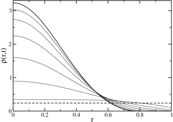
Figure 21: Evolution of the density profile $\rho(r,t)$ for $n=3/2$ and $\Theta=0.1$ (corresponding to $\eta>\omega_{n}$). The profile converges to a complete polytrope strictly confined inside the box (thick line). The dashed line is the initial uniform density profile.

We first consider the dynamics in the canonical ensemble (fixed $\Theta$). In Fig. 21, we show the different steps of the formation of a self-confined polytrope of index $n=3/2<n_{3}=3$ similar to a classical “white dwarf” star. In this range of $n$, the system always converges to an equilibrium state (see Fig. 15). If $\eta<\omega_{n}$ the equilibrium state is confined by the box (incomplete polytrope) while for $\eta>\omega_{n}$ the density vanishes at $R_{*}<R$ (complete polytrope). In Fig. 22, we illustrate the collapse dynamics at low temperatures for $n=4\in[n_{3},n_{5}]$ and $n=\infty>n_{5}=5$. This is compared to the predicted scaling profiles. The convergence to scaling is slower for $n=4$ ($\alpha=8/3$) than for $n=\infty$ ($\alpha=2$). This is expected since, in the former case, $r_{0}\sim\rho_{0}^{-1/\alpha}$ decreases more slowly as $\alpha$ is bigger. Thus, the scaling regime $r_{0}\ll 1$ is reached in a slower way. For instance, for comparable final densities of order $10^{6}$, and for the considered temperatures, we find that the minimum $r_{0}$ obtained for $n=4$ is roughly 4 times bigger than in the $n=\infty$ simulations. For $n=\infty$ and in the large $D$ limit, we have shown in [3] that the scaling function $S(x)$ takes the form

(202) $$S(x)=\frac{\alpha}{D}\left[1+\left(1-\frac{\alpha}{2z}\right)\left(\frac{x^{2}}{x_{0}^{2}}-1\right)\left(\frac{x^{2}}{x_{1}^{2}}+1\right)^{\frac{\alpha}{2}-1}\right]^{-1},$$

where $x_{0}$ is such that $S(x_{0})=\alpha/D$. The quantities $z=DS(0)/2$ and $\alpha(z)$ have been exactly calculated in this limit. In the present case, and for a given $n$ (yielding $\alpha_{n}=2n/(n-1))$, we compute $S(0)$, by assuming the above functional form. The parameter $x_{0}$, $x_{1}$ and $S(0)$ are numerically calculated by imposing the exact value for $S^{\prime\prime}(0)$ extracted from Eq. (181), as well as the two conditions that $x_{0}$ must satisfy (see [3] for more details). The comparison of this approximate theory with actual numerical data is satisfactory (see Fig. 23). Note that we have been unable to develop a large $n$ perturbation theory in the same spirit as the large $D$ expansion scheme derived in [3].

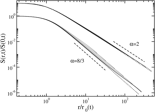
Figure 22: For $n=4$ ($\alpha_{4}=8/3$) and $\Theta=0.1$ (canonical description), we plot $S(r,t)/S(0,t)$ as a function of $r/r_{0}(t)$, where $r_{0}(t)$ is defined by Eq. (173), for different times corresponding to central densities in the range $2.10^{2}\sim 4.10^{5}$ (bottom data collapse). This is compared to the scaling function obtained by solving Eq. (181) numerically (dotted line). The same is plotted in the case $n=\infty$ ($\alpha_{\infty}=2$), for which the scaling profile is known analytically [3] : $S(x)/S(0)=(1+x^{2})^{-1}$ (upper data collapse). The two curves have been shifted for clarity. In the $n=\infty$ case, the asymptotic scaling profile (dotted line) is almost indistinguishable from the data collapse. Dashed lines have respective slopes $-8/3$ and $-2$.

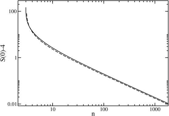
Figure 23: We plot $S(0)$ as a function of $n$ (full line), and compare it to a simple theory explained in the text, which is inspired by the large $D$ perturbation introduced in [3] (dashed line). Note that $S(0)\simeq 4+{C/n}+O(n^{-2})$ for large $n$ with $C\simeq 19$.

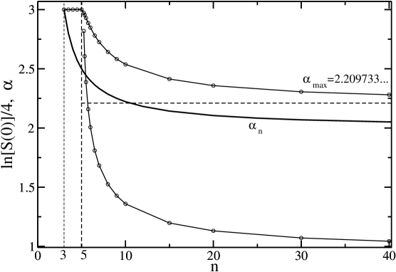
Figure 24: We plot $\alpha_{\rm max}(D=3,n)$ as a function of $n$ (top plot), as well as the associated value of $\frac{1}{4}\ln S(0)$ (bottom plot). The horizontal dashed line represents the asymptotic value of $\alpha_{\rm max}$ for $n\to+\infty$, and we find $\alpha_{\rm max}(D=3,n)\approx\alpha_{\rm max}(D=3,n=\infty)+C_{3}/n+O(n^{-2})$ for large $n$, with $C_{3}\sim 2.7$. For $n\leq n_{5}=5$, $\alpha_{\rm max}=D^{-}=3^{-}$ (strictly speaking, the scaling solution associated to $\alpha=D=3$ does not exist below $n_{5}=5$). We observe that $\ln S(0)\sim(n-5)^{-1/4}$ provides an excellent fit of $S(0)$ for $n\in[5,10]$. We have also plotted $\alpha_{n}=2n/(n-1)$ (thick line). The scaling equation (181) admits solutions for $\alpha_{n}\leq\alpha\leq\alpha_{\rm max}$. The two curves intersect when $\alpha_{n}=D$ which corresponds to $n=n_{3}$. There is no scaling collapse solution for $n\leq n_{3}$.

As explained in the previous section, the situation in the microcanonical ensemble (where $\Theta=\Theta(t)$ evolves with time in order to conserve energy) is less clear. Like in the case $n=\infty$ studied in [3], the scaling equation admits a physical solution for any $\alpha_{n}\leq\alpha\leq\alpha_{\rm max}(D,n)$. In Fig. 24, we plot $\alpha_{\rm max}(D=3,n)$, as well as the corresponding value of $S(0)$, as a function of $n$. As explained previously, it is doubtful that a scaling actually develops with $\alpha>\alpha_{n}$ when the temperature is uniform. However, a pseudo-scaling should be observed with $\alpha\simeq\alpha_{\rm max}$. In Fig. 25, we present new simulations ($D=3$, $n=\infty$) confirming that the observed scaling dynamics is better described by $\alpha=\alpha_{\rm max}$ than by $\alpha=2$, in the time/density range achieved. Such a value of $\alpha$ implies that the temperature would diverge with a small exponent ($\Theta(t)\sim\rho_{0}(t)^{1-2/\alpha_{{\rm max}}}$, with $1-2/\alpha_{\rm max}=0.09491...$). However, in the range of accessible densities $\rho_{0}=2.10^{-1}\sim 10^{6}$, numerical data tend to suggest that the temperature converges to a finite value with an infinite derivative $\frac{d\Theta}{dt}(t_{coll})=+\infty$ as $t\to t_{coll}$. This convergence of the temperature has been observed independently by [9]. Thus, we conclude that the system first develops an apparent scaling with $\alpha\lesssim\alpha_{\rm max}$, before slowly approaching the asymptotic scaling regime with $\alpha=2$. In any case, it is clear that if the $\alpha=2$ scaling is the relevant one, the scaling regime is approached much more slowly than in the canonical ensemble (compare Fig. 25 and Fig. 22). This is a new aspect of the inequivalence of statistical ensembles for self-gravitating systems.

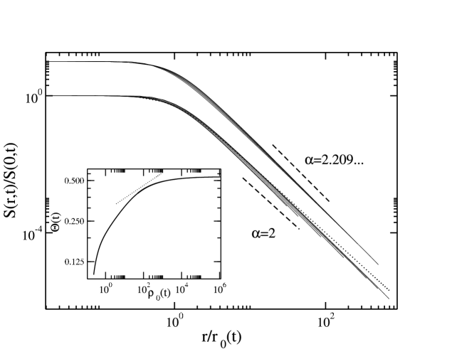
Figure 25: For $n=+\infty$ and $E=-0.45$ (microcanonical description), we plot $S(r,t)/S(0,t)$ as a function of $r/r_{0}(t)$ where $r_{0}(t)\sim\rho_{0}(t)^{1/\alpha}$, for times corresponding to central densities in the range $2.10^{2}\sim 4.10^{5}$ (for comparison, our previous simulations [2] did not exceed $\rho_{0}\sim 1000$). We try both values $\alpha_{\infty}=2$ (bottom plot) and $\alpha=\alpha_{\rm max}=2.209733...$ (top plot), and compare both data collapses to the associated scaling function (dotted lines). The two curves have been shifted for clarity. The scaling associated to $\alpha_{\rm max}$ is clearly more convincing than that for $\alpha=2$, especially at large distances. However, our simulations also suggest that $\Theta(t)\sim\rho_{0}(t)^{1-2/\alpha_{\rm max}}$ does not diverge at $t_{coll}$ (see the insert where a line of slope $1-2/\alpha_{\rm max}\approx 0.09491...$ has been drawn as a guide to the eye), so that the asymptotic scaling should correspond to $\alpha=2$. This apparent “paradox” clearly shows that the convergence to the limit value $\alpha=\alpha_{n}$ is extremely slow, suggesting an intermediate pseudo-scaling regime with $\alpha_{n}\leq\alpha\leq\alpha_{\rm max}$.

6 Conclusion

In this paper, we have discussed the structure and the stability of self-gravitating polytropic spheres by using a formalism of generalized thermodynamics [20]. This formalism allows us to present and organize the results in an original manner. What we mean by generalized thermodynamics is the extension of the usual variational principle of ordinary thermodynamics (maximization of the Boltzmann entropy $S_{B}$ at fixed mass $M$ and energy $E$) to a larger class of functionals (playing the role of “generalized entropies”). This variational problem can arise in various domains of physics (or biology, economy,…) for different reasons. In any case, it is relevant to develop a thermodynamical analogy and use a vocabulary borrowed from thermodynamics (entropy, temperature, chemical potential, caloric curve, free energy, microcanonical and canonical ensembles,…) even if the initial problem giving rise to this variational problem is not directly connected to thermodynamics. Thus, we can directly transpose the methods developed in the context of ordinary thermodynamics (e.g., Legendre transforms, turning point arguments, bifurcations,…) to a new context. For example, in the present study, the maximization of Tsallis entropy at fixed mass and energy is a condition of nonlinear dynamical stability for stellar polytropes via the Vlasov equation and for polytropic vortices via the Euler equation. On the other hand, the minimization of Tsallis free energy at fixed mass is connected to the nonlinear dynamical stability of polytropic stars via the Euler-Jeans equations. It is also a condition of thermodynamical stability (in a generalized sense) for self-gravitating Langevin particles experiencing anomalous diffusion and a condition of dynamical stability for bacterial populations. Although the formalism is the same for all these systems, the results have a very different physical interpretation. Our results may also have unexpected applications in other domains of physics that we are not aware of.

On a technical point of view, we have provided the complete equilibrium phase diagram of self-gravitating polytropic spheres for arbitrary value of the polytropic index $n$ and space dimension $D$. Our study, generalizing the classical study of Emden [49] and Chandrasekhar [18], shows how the phase portraits previously reported in the literature (for particular dimensions and particular polytropic indices) connect to each other in the full parameter space. From the geometrical structure of the generalized caloric curves, we can immediately determine the domains of stability of the polytropic spheres by using the turning point method [41]. These stability results have been confirmed by explicitly evaluating the second order variations of entropy and free energy. This eigenvalue method provides, in addition, the form of the density profile that triggers the instability at the critical points. Interestingly, this study can be performed analytically or by using simple graphical constructions in the Milne plane. We have found that complete stellar polytropes (with $n<n_{5}=(D+2)/(D-2)$ if $D>2$) are stable for $D\leq 4$ and unstable for $D>4$. On the other hand, complete gaseous polytropes are stable for $D\leq 2$ and for ($D>2$, $n\leq n_{3}=D/(D-2)$) and unstable for ($D>2$, $n>n_{3}$). Polytropes with index $n_{3/2}=D/2$ correspond to classical white dwarf stars (i.e., a self-gravitating Fermi gas at $T=0$). They are self-confined only for $D<2(1+\sqrt{2})$ and they are stable only for $D<4$. For $D>4$, quantum mechanics is not able to prevent gravitational collapse, even in the non-relativistic regime. In this sense, $D=4$ is a critical dimension. Therefore, our dimension of space $2<D=3<4$ is bounded by two critical dimensions. It seems that this remark has never been made before. The description of phase transitions in the self-gravitating Fermi gas at non-zero temperature in dimension $D$ will be considered in a future article [50]. Other possible extensions of our work would be to consider different equations of state such as the modified isothermal $p=-T\ln(1-\rho/\rho_{0})$ associated with an “entropy” functional $S[\rho]=-\int\{\rho\ln\rho+(\rho_{0}-\rho)\ln(\rho_{0}-\rho)\}d^{D}{\bf r}$ or the logotropic equation of state $p=p_{c}[1+A\ln(\rho/\rho_{c})]$ [51] associated with $S[\rho]=p_{c}A\int\ln\rho d^{D}{\bf r}$.

The concept of generalized thermodynamics is rigorously justified in the case of stochastic (Langevin) particles experiencing anomalous diffusion. This happens when the diffusion coefficient in the Fokker-Planck equation depends on the density of particles while the friction or drift is constant. In this paper, we have explicitly studied the nonlinear Smoluchowski-Poisson system (for self-gravitating Langevin particles) corresponding to a power-law dependance of the diffusion coefficient. This particular situation is connected to Tsallis generalized thermodynamics but more general Fokker-Planck equations can be constructed and studied [20]. The connection between thermodynamical and dynamical stability for this type of generalized Fokker-Planck equations has been established in the general case in [20]. The nonlinear Smoluchowski-Poisson system can have physical applications for the chemotaxis of bacterial populations. The collapse and aggregation of bacterial populations is similar, in some respect, to the phenomenon of core collapse in globular clusters (or to the Jeans instability in molecular clouds) and the neglect of inertia is rigorously justified in biology at variance with astrophysics. In addition, biological systems are likely to experience anomalous diffusion so that the NSP system can provide an interesting and relevant model for the problem of chemotaxis. We have shown that the solutions of the NSP system can either converge toward a complete polytrope or an incomplete polytrope restrained by the box, or lead to a situation of collapse. The determination of the scaling exponent $\alpha$ in the microcanonical ensemble (constant energy) is difficult due to the extremely slow entry of the system in the scaling regime. However, it seems to be given asymptotically by $\alpha_{n}=2n/(n-1)$ ($\alpha=2$ for isothermal spheres) as in the canonical ensemble (constant temperature). We expect that an exponent $\alpha>\alpha_{n}$ will be selected when the temperature is allowed to vary in space and time. This problem will be considered in a future study [30].

Appendix A Gravitational force in $D$ dimensions

The gravitational field produced in ${\bf r}$ by a distribution of $N$ particles with mass $m$ in a space of dimension $D$ is

(203) $${\bf F}=-\sum_{i=1}^{N}Gm{{\bf r}-{\bf r}_{i}\over|{\bf r}-{\bf r}_{i}|^{D}}.$$

For $D=1$, the gravitational field created by a particle is independent on the distance. Thus, an object located in $x$ experiences a force (by unit of mass) $F=Gm(N^{+}-N^{-})$, where $N^{+}$ is the number of particles in its right ($x_{i}>x$) and $N^{-}$ the number of particles in its left ($x_{i}<x$).

The external gravitational field created by a spherically symmetric distribution of matter with mass $M$ is

(204) $${\bf F}=-\nabla\Phi=-{GM\over r^{D-1}}{\bf e}_{r}.$$

For $D\neq 2$, the gravitational potential is

(205) $$\Phi=-{GM\over(D-2)r^{D-2}},$$

where the constant of integration has been taken equal to zero (this implies $\Phi=0$ at infinity for $D>2$). For $D=2$, we have,

(206) $$\Phi=GM\ln(r/R),$$

where we have taken $\Phi(R)=0$.

Appendix B Virial theorem in $D$ dimensions

We define the Virial of the gravitational force in dimension $D$ by

(207) $${\cal V}_{D}=\int\rho\ {\bf r}\cdot\nabla\Phi\ d^{D}{\bf r}.$$

For a spherically symmetric system, the Gauss theorem can be written

(208) $${d\Phi\over dr}={GM(r)\over r^{D-1}},\qquad M(r)=\int_{0}^{r}\rho S_{D}r^{{}^{\prime}D-1}dr^{\prime}.$$

Therefore, the Virial is equivalent to

(209) $${\cal V}_{D}=\int_{0}^{R}{dM\over dr}{GM(r)\over r^{D-2}}dr={G\over 2}\int_{0}^{R}{dM^{2}\over dr}{1\over r^{D-2}}dr.$$

In $D=2$, one has directly

(210) $${\cal V}_{2}={GM^{2}\over 2}.$$

If now $D\neq 2$, we obtain after an integration by parts

(211) $${\cal V}_{D}={GM^{2}\over 2R^{D-2}}+{1\over 2}(D-2)\int_{0}^{R}{GM(r)^{2}\over r^{D-1}}dr,$$

or, using Eq. (208),

(212) $${\cal V}_{D}={GM^{2}\over 2R^{D-2}}+{1\over 2G}(D-2)\int_{0}^{R}{\biggl{(}{d\Phi\over dr}\biggr{)}^{2}}r^{D-1}dr.$$

Now, using the Poisson equation (4), the potential energy can be written

(213) $$W={1\over 2}\int\rho\Phi d^{D}{\bf r}={1\over 2S_{D}G}\int\Phi\Delta\Phi d^{D}{\bf r}.$$

Integrating by parts, we obtain

(214) $$W={1\over 2S_{D}G}\biggl{\{}\Phi(R){d\Phi\over dr}(R)S_{D}R^{D-1}-\int_{0}^{R}\biggl{(}{d\Phi\over dr}\biggr{)}^{2}r^{D-1}S_{D}dr\biggr{\}}.$$

The gravitational force and the gravitational potential at the edge of the box are given by Eqs. (204) and (205). Introducing these results in Eq. (214) and comparing with Eq. (212), we obtain

(215) $${\cal V}_{D}=-(D-2)W,\qquad D\neq 2.$$

By using the Virial tensor method introduced by Chandrasekhar [19], we can show that the foregoing relation remains valid if the system is not spherically symmetric.

If now the system is in hydrostatic equilibrium, we have

(216) $$\nabla p=-\rho\nabla\Phi.$$

Inserting this relation in the Virial (207) and integrating by parts, we get

(217) $${\cal V}_{D}=-\oint p\ {\bf r}\cdot d{\bf S}+2K,$$

where we have used $K=(D/2)\int pd^{D}{\bf r}$. This is the expression of the Virial theorem in its general form. Assuming now that $p_{b}$ is uniform on the domain boundary (which is true at least for a spherically symmetric system), we have

(218) $$\oint p\ {\bf r}\cdot d{\bf S}=p_{b}\oint{\bf r}\cdot d{\bf S}=p_{b}\int\nabla\cdot{\bf r}\ d^{D}{\bf r}=p_{b}DV_{D}R^{D}.$$

Therefore, for a spherically symmetric system, the Virial theorem reads

(219) $$2K-{\cal V}_{D}=p(R)DV_{D}R^{D},$$

where ${\cal V}_{D}$ is given by Eqs. (210) and (215).

It is interesting to consider a direct application of these results. In $D=2$, the Virial theorem reads

(220) $$2K-{GM^{2}\over 2}=2\pi R^{2}p(R).$$

For an isothermal gas $K=MT$ so that

(221) $$2MT-{GM^{2}\over 2}=2\pi R^{2}p(R).$$

From this relation, we conclude that there exists an equilibrium solution with $p(R)=0$ at $T_{c}=GM/4$. We therefore recover the critical temperature of an isothermal self-gravitating gas in two-dimensions (see, e.g., [3]). At $T=T_{c}$, the density profile is a Dirac peak so that $p(R)=0$. For $T<T_{c}$, there is no static solution and the system undergoes a gravitational collapse. This collapse was studied in [3] with the Smoluchowski-Poisson system.

Appendix C Special properties of $n_{3/2}$ polytropes

In this Appendix, we consider polytropes with index $n_{3/2}=D/2$ in a space of dimension $D\geq 4$. They correspond to $D$-dimensional “white dwarf” stars. According to Eq. (113), the curve $\eta(\alpha)$ is extremum for

(222) $$u_{0}={D(D-4)\over D-2}.$$

It is easy to check that this particular value is also solution of Eq. (117) determining maxima of $\Lambda(\alpha)$. We conclude therefore that the functions $\eta(\alpha)$ and $\Lambda(\alpha)$ achieve extremal values for the same values of $\alpha$ in the series of equilibria. This implies that the generalized caloric curve $\eta(\Lambda)$ of $n_{3/2}$ polytropes displays angular points (see Figs. 16 and 18).

Appendix D Second order variations of generalized entropy and free energy

According to Eq. (35), the variations of entropy up to second order are

(223) $$\delta S={D-2n\over 2}\biggl{(}\beta\int\delta pd^{D}{\bf r}+\delta\beta\int pd^{D}{\bf r}+\int\delta\beta\delta pd^{D}{\bf r}\biggr{)}.$$

On the other hand, according to the polytropic equation of state (30), we have

(224) $$\delta p=\gamma{\delta\rho\over\rho}p+{\gamma p\over n}{(\delta\rho)^{2}\over 2\rho^{2}}+{\delta K\over K}p+\gamma{\delta K\over K}{\delta\rho\over\rho}p.$$

From Eqs. (24) and (31),

(225) $$K\sim\beta^{D-2n\over 2n},$$

so that to second order

(226) $${\delta K\over K}={D-2n\over 2n}{\delta\beta\over\beta}+{(D-2n)(D-4n)\over 8n^{2}}\biggl{(}{\delta\beta\over\beta}\biggr{)}^{2}.$$

Inserting Eqs. (226) and (224) in Eq. (223), we get

$$\delta S={D-2n\over 2}\biggl{[}\beta\gamma\int{\delta\rho\over\rho}pd^{D}{\bf r}+{\beta\gamma\over 2n}\int{p\over\rho^{2}}(\delta\rho)^{2}d^{D}{\bf r}+{D\over 2n}\int p\delta\beta d^{D}{\bf r}$$

(227) $$+{\gamma D\over 2n}\delta\beta\int{\delta\rho\over\rho}pd^{D}{\bf r}+{D(D-2n)\over 8n^{2}}{(\delta\beta)^{2}\over\beta}\int pd^{D}{\bf r}\biggr{]}.$$

Now, the conservation of energy (34) implies that

(228) $$0=\delta E={D\over 2}\int\delta pd^{D}{\bf r}+{1\over 2}\int\delta\rho\delta\Phi d^{D}{\bf r}+\int\Phi\delta\rho d^{D}{\bf r}.$$

Inserting Eqs. (224) and (226) in Eq. (228), we obtain

$${D-2n\over 2}\biggl{[}{\gamma D\over D-2n}\beta\int{\delta\rho\over\rho}pd^{D}{\bf r}+{\gamma D\over 2n(D-2n)}\beta\int p{(\delta\rho)^{2}\over\rho^{2}}d^{D}{\bf r}+{D\over 2n}\int\delta\beta pd^{D}{\bf r}$$

$$+{D(D-4n)\over 8n^{2}}{(\delta\beta)^{2}\over\beta}\int pd^{D}{\bf r}+{\gamma D\over 2n}\delta\beta\int{\delta\rho\over\rho}pd^{D}{\bf r}\biggr{]}$$

(229) $$+{1\over 2}\beta\int\delta\rho\delta\Phi d^{D}{\bf r}+\beta\int\Phi\delta\rho d^{D}{\bf r}=0.$$

Subtracting this relation from Eq. (227), we get

$$\delta S=-\beta\gamma n\int{\delta\rho\over\rho}pd^{D}{\bf r}-{1\over 2}\beta\gamma\int p{(\delta\rho)^{2}\over\rho^{2}}d^{D}{\bf r}+{D(D-2n)\over 8n}{(\delta\beta)^{2}\over\beta}\int pd^{D}{\bf r}$$

(230) $$-{1\over 2}\beta\int\delta\rho\delta\Phi d^{D}{\bf r}-\beta\int\Phi\delta\rho d^{D}{\bf r}.$$

Now, to first order, Eq. (229) yields

(231) $${\delta\beta\over\beta}=-{4n\over D(D-2n)}{\int\Phi\delta\rho d^{D}{\bf r}+{D\over 2}\gamma\int{\delta\rho\over\rho}pd^{D}{\bf r}\over\int pd^{D}{\bf r}}.$$

Substituting this relation in Eq. (230), we find that the second order variations of entropy are given by Eq. (137). To compute the second order variations of free energy $F=E-TS$, we can use Eqs. (227) and (228) with $\delta\beta=0$. This yields Eq. (123).

Appendix E Some useful identities

In this Appendix, we establish the identities (147)-(149) that are needed in the stability analysis of Sec. 3.7. Using an integration by parts, we have

(232) $$\int_{0}^{\alpha}\theta^{\prime}\xi^{D}\theta^{n}d\xi=\int_{0}^{\alpha}\xi^{D}{d\over d\xi}\biggl{(}{\theta^{n+1}\over n+1}\biggr{)}d\xi={1\over n+1}\alpha^{D}\theta^{n+1}(\alpha)-{D\over n+1}\int_{0}^{\alpha}\xi^{D-1}\theta^{n+1}d\xi.$$

Using the Lane-Emden equation (45) and integrating by parts, we obtain

(233) $$\int_{0}^{\alpha}\theta^{n+1}\xi^{D-1}d\xi=-\alpha^{D-1}\theta(\alpha)\theta^{\prime}(\alpha)+\int_{0}^{\alpha}(\theta^{\prime})^{2}\xi^{D-1}d\xi.$$

Using the relation

(234) $$\int_{0}^{\alpha}{\xi^{1+D\over 2}\theta^{\prime}\over\xi}{d\over d\xi}\biggl{(}\xi^{1+D\over 2}\theta^{\prime}\biggr{)}d\xi=\alpha^{D}\theta^{\prime}(\alpha)^{2}-\int_{0}^{\alpha}{\xi^{1+D\over 2}\theta^{\prime}\over\xi}{d\over d\xi}\biggl{(}\xi^{1+D\over 2}\theta^{\prime}\biggr{)}d\xi+\int_{0}^{\alpha}\xi^{D-1}(\theta^{\prime})^{2}d\xi,$$

which results from a simple integration by parts, we get

(235) $$\int_{0}^{\alpha}\xi^{D-1}(\theta^{\prime})^{2}d\xi=-\alpha^{D}\theta^{\prime}(\alpha)^{2}+2\int_{0}^{\alpha}\xi^{D-1\over 2}{d\over d\xi}\biggl{(}\xi^{1+D\over 2}\theta^{\prime}\biggr{)}\theta^{\prime}d\xi,$$

or, equivalently,

(236) $$D\int_{0}^{\alpha}\xi^{D-1}(\theta^{\prime})^{2}d\xi=\alpha^{D}\theta^{\prime}(\alpha)^{2}-2\int_{0}^{\alpha}\xi^{D}\theta^{\prime\prime}\theta^{\prime}d\xi.$$

Using the Lane-Emden equation (45), we find that

(237) $$(D-2)\int_{0}^{\alpha}\xi^{D-1}(\theta^{\prime})^{2}d\xi=-\alpha^{D}\theta^{\prime}(\alpha)^{2}-2\int_{0}^{\alpha}\xi^{D}\theta^{\prime}\theta^{n}d\xi.$$

We have three equations (232), (233) and (237) for three unknown integrals. Solving this system of algebraic equations and introducing the Milne variables (70), we obtain the identities (147)-(149).

Appendix F Dynamical stability of gaseous spheres

In this section, we assume $D>2$. According to Eq. (37), the energy of a polytropic star at equilibrium (${\bf u}={\bf 0}$) can be written

(238) $${\cal W}={2n\over D}K+W,$$

where $K$ is the kinetic energy and $W$ the potential energy. Now, for a complete polytrope ($p_{b}=0$), the Virial theorem reads

(239) $$2K+(D-2)W=0.$$

Combining the foregoing relations, we get

(240) $${\cal W}=\biggl{(}1-{n\over n_{3}}\biggr{)}W.$$

According to Poincaré’s theorem, a gaseous star with ${\cal W}>0$ is unstable [18]. For polytropic stars, this condition is equivalent to $n>n_{3}$.

More generally, the internal energy of a mass $dm$ of gas at temperature $T$ is $dU=C_{v}dmT$. Its kinetic energy is $dK={D\over 2}dmRT={D\over 2}(C_{p}-C_{v})dmT$ where $R$ is the constant of perfect gases and $C_{v}$, $C_{p}$ are the specific heats at constant volume and constant pressure, respectively. Thus, we get

(241) $$U={2\over D(\gamma-1)}K,$$

where $\gamma=C_{p}/C_{v}$. For a monoatomic gas, $\gamma=(D+2)/D$ and $U=K$. Using the Virial theorem (239), the total energy of the star ${\cal W}=U+W$ can be written

(242) $${\cal W}={D\gamma-2(D-1)\over D(\gamma-1)}W.$$

The star is unstable for $\gamma<\gamma_{crit}=2(D-1)/D$. For $D=3$, we recover the well-known result $\gamma_{crit}=4/3$. For a polytropic gas, we recover the result $\gamma_{crit}=1+1/n_{3}$.

References

- [1] P.H. Chavanis, J. Sommeria and R. Robert, Astrophys. J. 471, 385 (1996).
- [2] P.H. Chavanis, C. Rosier and C. Sire, Phys. Rev. E, 66, 6105 (2002).
- [3] C. Sire and P.H. Chavanis, Phys. Rev. E, 66, 6133 (2002).
- [4] C. Sire and P.H. Chavanis, submitted to Phys. Rev. E [cond-mat/0306406].
- [5] M.A. Herrero, E. Medina, J.J.L. Velazquez, J. Comput. Appl. Math., 97, 99 (1998).
- [6] P. Biler, G. Karch, J. Dolbeault and M.J. Esteban, Adv. Diff. Eqs., 6, 461 (2001).
- [7] C. Rosier, C.R. Acad. Sci., Ser. I: Math., 332, 903 (2001).
- [8] P. Biler and T. Nadzieja, preprint.
- [9] I.A. Guerra, M.A. Peletier and J. Williams, preprint.
- [10] H. Risken, The Fokker-Planck equation (Springer, 1989).
- [11] J.D. Murray, Mathematical Biology (Springer, 1991).
- [12] R. Robert and J. Sommeria, Phys. Rev. Lett. 69, 2776 (1992).
- [13] P.H. Chavanis, Phys. Rev. E 58, R1199 (1998).
- [14] P.H. Chavanis, Phys. Rev. Lett. 84, 5512 (2000).
- [15] P.H. Chavanis, Phys. Rev. E 64, 6309 (2001).
- [16] P.H. Chavanis in Dynamics and Thermodynamics of Systems with Long Range Interactions, edited by T. Dauxois, S. Ruffo, E. Arimondo, M. Wilkens, (Lecture Notes in Physics Vol. 602, Springer 2002) [cond-mat/0212223].
- [17] P.H. Chavanis, [cond-mat/0209098].
- [18] S. Chandrasekhar, An introduction to the theory of stellar structure (Dover, 1939).
- [19] J. Binney and S. Tremaine, Galactic Dynamics (Princeton Series in Astrophysics, 1987).
- [20] P.H. Chavanis, Phys. Rev. E, in press [cond-mat/0209096].
- [21] L. Borland, Phys. Rev. E 57, 6634 (1998).
- [22] G. Kaniadakis, Physica A 296, 405 (2001).
- [23] P.H. Chavanis, Physica A, in press [cond-mat/0304073].
- [24] M. Shiino, Phys. Rev. E 67, 6118 (2003).
- [25] C. Tsallis, J. Stat. Phys. 52, 479 (1988).
- [26] P.H. Chavanis, Astron. Astrophys. 401, 15 (2003).
- [27] A. Taruya and M. Sakagami, Physica A 307, 185 (2002).
- [28] A. Taruya and M. Sakagami, Physica A, 318, 387 (2003).
- [29] P.H. Chavanis, Astron. Astrophys. 386, 732 (2002).
- [30] C. Sire and P.H. Chavanis, in preparation.
- [31] P.H. Chavanis, Ann. N.Y. Acad. Sc. 867, 120 (1998).
- [32] P.H. Chavanis, in: Proceedings of the Conference on Multiscale Problems in Science and Technology, edited by N. Antonic, C.J. van Duijn, W. Jäger and A. Mikelic (Springer 2002) [astro-ph/0212205].
- [33] J.R. Ipser and G. Horwitz, ApJ 232, 863 (1979).
- [34] S. Tremaine, M. Hénon and D. Lynden-Bell, Mon. Not. R. astr. Soc. 219 285 (1986).
- [35] P.H. Chavanis and M. Rieutord, A&A, in press [astro-ph/0302594].
- [36] G. Joyce and D. Montgomery, J. Plasma Phys. 10, 107 (1973).
- [37] R. Ellis, K. Haven and B. Turkington, Nonlinearity 15, 239 (2002).
- [38] F. Bouchet, PhD thesis, Université J. Fourier (2001).
- [39] Y.Y. Yamaguchi, J. Barré, F. Bouchet, T. Dauxois & S. Ruffo, in preparation.
- [40] H.C. Plummer, Mon. Not. R. astr. Soc. 71, 460 (1911).
- [41] J. Katz, Mon. Not. R. astr. Soc. 183, 765 (1978).
- [42] T. Padmanabhan, Phys. Rep. 188, 285 (1990).
- [43] P.H. Chavanis, M. Ribot, C. Rosier and C. Sire, in preparation.
- [44] P.H. Chavanis, Astron. Astrophys. 356, 1089 (2000).
- [45] D. Lynden-Bell and R. Wood, Mon. Not. R. astr. Soc. 138, 495 (1968).
- [46] R.B. Larson, Mon. Not. R. astr. Soc. 147, 323 (1970).
- [47] H. Cohn, Astrophys. J. 242, 765 (1980).
- [48] D. Lynden-Bell and P.P. Eggleton, Mon. Not. R. astr. Soc. 191, 483 (1980).
- [49] R. Emden, Gaskugeln (Teubner Verlag, Leipzig, 1907).
- [50] P.H. Chavanis, in preparation.
- [51] D.E. McLaughlin and R.E. Pudritz, ApJ 476, 750 (1997).