Droplet Spreading on Heterogeneous Surfaces
using a Three-Dimensional
Lattice Boltzmann Model

Abstract

We use a three-dimensional lattice Boltzmann model to investigate the spreading of mesoscale droplets on homogeneous and heterogeneous surfaces. On a homogeneous substrate the base radius of the droplet grows with time as $t^{0.28}$ for a range of viscosities and surface tensions. The time evolutions collapse onto a single curve as a function of a dimensionless time. On a surface comprising of alternate hydrophobic and hydrophilic stripes the wetting velocity is anisotropic and the equilibrium shape of the droplet reflects the wetting properties of the underlying substrate.

1 Introduction

Wetting processes, such as the spreading of a droplet over a surface, have attracted the attention of scientists for a long time [1]. A great deal is understood about the wetting behaviour of equilibrium droplets. However less is known about the dynamics of these systems, a problem of considerable industrial relevance with the advent of ink-jet printing. The droplets involved in printing typically have length scales of microns. Experimental work on such mesoscopic droplets is difficult and expensive because of the length- and time-scales involved. Therefore there is a need for numerical modelling both to investigate the physics and to help design and interpret the experiments.

Lattice Boltzmann models are a class of numerical techniques ideally suited to probing the behaviour of fluids on mesoscopic length scales [2]. Several lattice Boltzmann algorithms for a liquid-gas system have been reported in the literature [3, 4, 5]. They solve the Navier-Stokes equations of fluid flow but also input thermodynamic information, typically either as a free energy or as effective microscopic interactions. They have proved successful in modelling such diverse problems as fluid flows in complex geometries [6], two-phase models [3, 4], hydrodynamic phase ordering [7] and sediment transport in a fluid [8].

Here we show that it is possible to use a lattice Boltzmann approach to model the spreading of mesoscale droplets and, in particular, to illustrate how a droplet spreads on a substrate comprising of hydrophilic and hydrophobic stripes.

We consider a one-component, two-phase fluid and use the free energy model originally described by Swift et al. [3] with a correction to ensure Galilean invariance [9]. The advantage of this approach for the wetting problem is that it allows us to tune equilibrium thermodynamic properties such as the surface tension or static contact angle to agree with analytic predictions. Thus it is rather easy to control the wetting properties of the substrate. Three dimensional simulations of spreading on smooth and rough substrates have previously been reported in [10] using a different lattice Boltzmann algorithm.

The paper is organised as follows. First we summarise the main features of the lattice Boltzmann approach. The model is validated by showing the consistency of the measured equilibrium contact angle with that predicted by Young’s law and by measuring the base radius of the spreading droplet as a function of time obtaining, as expected, a power law growth. We show that when the reduced base radius is plotted as a function of reduced time the data fall on a universal curve for several values of surface tension and viscosity.

We then consider spreading on a heterogeneous substrate consisting of alternate hydrophobic and hydrophilic stripes. We find that the spreading velocity is anisotropic and that the final droplet shape reflects the wetting properties of the underlying substrate. Finally, a conclusion suggests extensions to the work presented here.

2 Simulating spreading

2.1 The lattice Boltzmann model

The lattice Boltzmann approach solves the Navier-Stokes equations by following the evolution of partial distribution functions $f_{i}$ on a regular, $d$-dimensional lattice formed of sites $\mathbf{r}$. The label $i$ denotes velocity directions and runs between $0$ and $z$. $DdQz+1$ is a standard lattice topology classification. The $D3Q15$ lattice topology we use here has the following velocity vectors $\mathbf{v}_{i}$: $(0,0,0)$, $(\pm 1,\pm 1,\pm 1)$, $(\pm 1,0,0)$, $(0,\pm 1,0)$, $(0,0,\pm 1)$ in lattice units.

The lattice Boltzmann dynamics are given by

$$f_{i}(\mathbf{r}+\Delta t\mathbf{v}_{i},t+\Delta t)=f_{i}(\mathbf{r},t)+\frac{1}{\tau}\left(f_{i}^{eq}(\mathbf{r},t)-f_{i}(\mathbf{r},t)\right)$$ (1)

where $\Delta t$ is the time step of the simulation, $\tau$ the relaxation time and $f_{i}^{eq}$ the equilibrium distribution function which is a function of the density $n=\sum_{i=0}^{z}f_{i}$ and the fluid velocity $\mathbf{u}$ defined through the relation $n\mathbf{u}=\sum_{i=0}^{z}f_{i}\mathbf{v}_{i}$.

The relaxation time tunes the kinematic viscosity as

$$\nu=\frac{\Delta\mathbf{r}^{2}}{\Delta t}\frac{C_{4}}{C_{2}}(\tau-\frac{1}{2})$$ (2)

where $\Delta\mathbf{r}$ is the lattice spacing and $C_{2}$ and $C_{4}$ are coefficients related to the topology of the lattice. These are equal to $3$ and $1$ respectively when one considers a $D3Q15$ lattice (see [11] for more details).

It can be shown [3] that equation (1) reproduces the Navier-Stokes equations of a non-ideal gas if the local equilibrium functions are chosen as

$$f_{i}^{eq} = A_{\sigma}+B_{\sigma}u_{\alpha}v_{i\alpha}+C_{\sigma}\mathbf{u}^{2}+D_{\sigma}u_{\alpha}u_{\beta}v_{i\alpha}v_{i\beta}+G_{\sigma\alpha\beta}v_{i\alpha}v_{i\beta},\quad i>0,$$

$$f_{0}^{eq} = n-\sum_{i=1}^{z}f_{i}^{eq}$$ (3)

where Einstein notation is understood for the Cartesian labels $\alpha$ and $\beta$ (i.e. $v_{i\alpha}u_{\alpha}=\sum_{\alpha}v_{i\alpha}u_{\alpha}$) and where $\sigma$ labels velocities of different magnitude.

The coefficients $A_{\sigma}$, $B_{\sigma}$, $C_{\sigma}$, $D_{\sigma}$ and $G_{\sigma}$ are chosen so as to satisfy the relations

$$\sum_{i}f_{i}^{eq} = n,$$

$$\sum_{i}f_{i}^{eq}v_{i\alpha} = nu_{\alpha},$$

$$\sum_{i}f_{i}^{eq}v_{i\alpha}v_{i\beta} = P_{\alpha\beta}+nu_{\alpha}u_{\beta}+\nu\left(u_{\alpha}\partial_{\beta}n+u_{\beta}\partial_{\alpha}n+u_{\gamma}\partial_{\gamma}n\delta_{\alpha\beta}\right),$$

$$\sum_{i}f_{i}^{eq}v_{i\alpha}v_{i\beta}v_{i\gamma} = \frac{c^{2}n}{3}(u_{\alpha}\delta_{\beta\gamma}+u_{\beta}\delta_{\alpha\gamma}+u_{\gamma}\delta_{\alpha\beta})$$ (4)

where $P_{\alpha\beta}$ is the pressure tensor, $c$ is defined to be $\Delta\mathbf{r}/\Delta t$ and the last term of the third expression in equation (4) is included to ensure Galilean invariance.

Considering a $D3Q15$ lattice and a square-gradient approximation to the interface free energy ($\kappa(\partial_{\alpha}n)^{2}/2$) [3], a possible choice of the coefficients is [12]

$$A_{\sigma} = \frac{w_{\sigma}}{c^{2}}\left(p_{b}-\frac{\kappa}{2}(\partial_{\alpha}n)^{2}-\kappa n\partial_{\alpha\alpha}n+\nu u_{\alpha}\partial_{\alpha}n\right),$$

$$B_{\sigma} = \frac{w_{\sigma}n}{c^{2}},\quad C_{\sigma}=-\frac{w_{\sigma}n}{2c^{2}},\quad D_{\sigma}=\frac{3w_{\sigma}n}{2c^{4}},$$

$$G_{1\gamma\gamma} = \frac{1}{2c^{4}}\left(\kappa(\partial_{\gamma}n)^{2}+2\nu u_{\gamma}\partial_{\gamma}n\right),\quad G_{2\gamma\gamma}=0,$$

$$G_{2\gamma\delta} = \frac{1}{16c^{4}}\left(\kappa(\partial_{\gamma}n)(\partial_{\delta}n)+\nu(u_{\gamma}\partial_{\delta}n+u_{\delta}\partial_{\gamma}n)\right)$$ (5)

where $w_{1}=1/3$, $w_{2}=1/24$, $\kappa$ is a parameter related to the surface tension and $p_{b}$ is the pressure in the bulk which is defined below. One can show [13] that the pressure tensor can be written as

$$P_{\alpha\beta}=\left(p_{b}-\frac{\kappa}{2}(\partial_{\gamma}n)^{2}-\kappa n\partial_{\gamma\gamma}n\right)\delta_{\alpha\beta}+\kappa(\partial_{\alpha}n)(\partial_{\beta}n).$$ (6)

2.2 Wetting boundary conditions

In this paper, we will focus our attention on flat substrates normal to the $z$ direction. The derivatives in that direction should then be handled in such a way that the wetting properties of the substrate can be controlled. A boundary condition can be established using the Cahn model [14]. He proposed adding an additional surface free energy $\Psi_{c}(n_{s})=\phi_{0}-\phi_{1}n_{s}+\cdots$ at the solid surface where $n_{s}$ is the density at the surface. Neglecting the second order terms of $\Psi_{c}(n)$ and minimizing $\Psi_{b}+\Psi_{c}$ (where $\Psi_{b}$ is the free energy in the bulk), a boundary condition valid at $z=0$ emerges [15]

$$\partial_{z}n=-\frac{\phi_{1}}{\kappa}.$$ (7)

Equation (7) is imposed on the substrate sites to implement the Cahn model in the lattice Boltzmann approach. Details are given in [15].

The Cahn model can be used to relate $\phi_{1}$ to $\theta$ the contact angle defined as the angle between the tangent plane to the droplet and the substrate. Within the Cahn model the surface tension at the interfaces is given by [1]

$$\sigma_{lg} = \int_{n_{g}}^{n_{l}}\sqrt{2\kappa W(n,T)}dn$$

$$\sigma_{sl,sg} = \left|\int_{n_{s}}^{n_{g,l}}\sqrt{2\kappa W(n,T)}dn\right|+\phi_{0}-\phi_{1}n_{s}$$ (8)

where $W(n,T)$ is the excess free energy, $\sigma_{lg}$, $\sigma_{sg}$, $\sigma_{sl}$ are the surface tensions at the liquid-gas, solid-gas and solid-liquid interface respectively and $n_{s}$, $n_{l}$, $n_{g}$ are the densities at the substrate, of the liquid phase and of the gas phase respectively. Young’s law [16] gives a relation between the static contact angle and the surface tensions of the three phases

$$\sigma_{lg}\cos\theta=\sigma_{sg}-\sigma_{sl}.$$ (9)

A convenient choice of bulk pressure is [15]

$$p_{b}=p_{c}(\nu_{p}+1)^{2}(3\nu_{p}^{2}-2\nu_{p}+1-2\beta\tau_{p})$$ (10)

where $\nu_{p}=(n-n_{c})/n_{c}$, $\tau_{p}=(T_{c}-T)/T_{c}$ and $p_{c}=1/8$, $n_{c}=3.5$ and $T_{c}=4/7$ are the critical pressure, density and temperature respectively and $\beta$ is a constant typically equal to $0.1$. The excess free energy then becomes [15]

$$W(n,T)=p_{c}(\nu_{p}^{2}-\beta\tau_{p})^{2}.$$ (11)

Inserting equation (11) into relation (8) and using equation (9), gives the relation between $\phi_{1}$ and $\theta$

$$\phi_{1}=2\beta\tau_{p}\sqrt{2p_{c}\kappa}\;\mathrm{sign}(\theta-\frac{\pi}{2})\sqrt{\cos\frac{\alpha}{3}\left(1-\cos\frac{\alpha}{3}\right)}$$ (12)

where $\alpha=\mathrm{cos}^{-1}(\sin^{2}\theta)$ and the function $\mathrm{sign}$ returns the sign of its argument.

We impose a no-slip boundary condition on the velocity. Because a collision takes place on the boundary the usual bounce-back condition must be extended to ensure mass conservation (see [11] for a wider discussion). This is done by a suitable choice of the rest field, $f_{0}$, to correctly balance the mass of the system.

3 Spreading on a homogeneous surface

We consider a $80\times 80\times 40$ lattice on which a spherical drop of radius $R_{0}=16$ just touches a flat surface at $z=0$. Unless otherwise specified the temperature is $T=0.4$ which leads to two phases of density $n_{l}=4.128$ and $n_{g}=2.913$. Fig. 1 shows how the droplet evolves in time to reach an equilibrium shape with contact angle $60^{\circ}$.

$t=0$	$t=250$	$t=500$
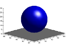
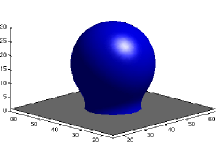
$t=1000$	$t=5000$	$t=20000$

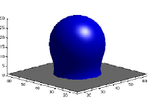
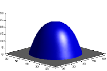
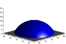
Figure 1: Spreading of a spherical droplet of radius $R_{0}=16$ on a $80\times 80\times 40$ lattice. The equilibrium contact angle is $60^{\circ}$.

We first present a check on the accuracy of the equilibrium properties of the model. Fig. 2 reports a comparison between two methods of measuring the contact angle. $\theta^{y}$ is the contact angle obtained from equation (9) with the surface tensions measured at equilibrium. $\theta^{g}$ is the contact angle measured from the profile of the simulated droplet once equilibrium is reached. The agreement is good. Small errors results from the difficulty of a direct measurement of the contact angle on a discrete lattice.

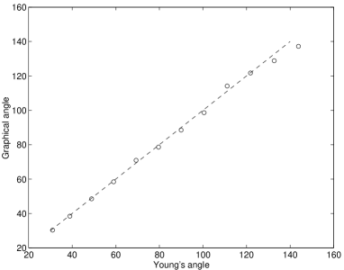
Figure 2: Comparison between equilibrium contact angles $\theta^{y}$ and $\theta^{g}$ (defined in the text) on a $110\times 110\times 50$ lattice. The input contact angles are set from $30^{\circ}$ to $140^{\circ}$ every $10^{\circ}$. $\tau=1.0$ and $\kappa=0.003$. The initial droplet has a radius $R_{0}=18$. $80~{}000$ iterations were used to reach each equilibrium. The dashed line is the expected agreement.

The shape of the area formed by the contact of a droplet with a homogeneous substrate is a disk. Its radius $R_{c}$ is a quantity which is rather simple to measure and has consequently attracted the attention of many scientists, see [17] and references therein. The time evolution of $R_{c}$ has been found to follow a power law $R_{c}=mt^{n/2}$. The exponent $n$ has been widely reported in the literature but with no consistent result. Marmur [17] in his review lists exponents between $0.06$ and $0.6$. The value of $m$ appears to be related to the droplet volume.

Fig. 3 shows the time evolution of $R_{c}$ for different values of the viscosity and the surface tension. The curves correspond to a value $n=0.56$ which is within the range reported in the literature. The power law is independent of the surface tension and the viscosity.

Indeed if the evolution curves are plotted as a function of the dimensionless time [18]

$$t\longrightarrow t^{*}=\frac{\sigma_{lg}}{\eta R_{0}}t$$ (13)

the data collapses onto a single curve as shown in fig. 3(b). Experimental data taken from [18] shows similar behaviour.

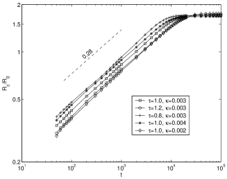
(a)	(b)

Figure 3: Time evolution of the radius of the droplet base $R_{c}$ on a $90\times 90\times 50$ lattice (a) as a function of time $t$ (b) as a function of dimensionless time $t^{*}$. The contact angle is set to $60^{\circ}$ and $R_{0}=16$. The solid line is the result of laboratory experiments [18].

4 Spreading on heterogeneous surfaces

Almost any surface will contain physical and chemical inhomogeneities which will affect the spreading of a mesoscopic droplet. It has recently become feasible to fabricate surfaces with well-defined chemical properties on micron length scales and it is becoming possible to perform well-controlled experiments which probe the behaviour of mesoscopic droplets on chemically and physically heterogeneous substrates. Thus it is particularly interesting to develop techniques to model the effect of these surfaces on the spreading properties of a droplet.

One of the simplest heterogeneous surfaces can be formed by alternating stripes of materials with different wetting properties. The static properties of droplets on such substrates have been discussed [19, 20, 21]. However less attention has been paid to the dynamics of the spreading.

In this section we consider heterogeneous surfaces formed by alternating hydrophilic and hydrophobic stripes. They are characterised by widths $w_{phi}$,$w_{pho}$ and contact angles $\theta_{phi}$, $\theta_{pho}$ respectively. Fig. 4 presents the behaviour of a three-dimensional droplet spreading on such a surface with $\theta_{phi}=50^{\circ}$, $\theta_{pho}=110^{\circ}$, $w_{phi}=6$, $w_{pho}=5$. The droplet has an initial radius $R_{0}=18$.

It is apparent from the figure that the behaviour of the droplet depends on whether it is on a hydrophobic or a hydrophilic stripe. The equilibrium shape of the contact line shown in fig. 4(b) reflects the pattern of the underlying substrate which is comparable to that found in laboratory experiments [20].

The time evolution of the contact line is also shown in fig. 4(b). Note that its velocity decreases smoothly in the $y$-direction parallel to the stripes but not in the $x$-direction where it moves faster on the hydrophilic than on the hydrophobic stripes. Note also that the droplet remains symmetric about an axis perpendicular to the stripes but that the shape becomes asymmetric about an axis parallel to the stripes, depending upon the initial position of the center of the droplet.

Observation of the movement of the contact line in the $x$-direction shows that in a hydrophilic region the contact angle tends to decrease and the velocity of the contact line increase. When the contact line reaches the boundary its progress is stopped and the contact angle increases until it is large enough to cross the hydrophobic stripe.

It has been proposed that an equilibrium droplet on such a surface has a spatially averaged contact angle following Cassie’s law [21]

$$\cos\theta=p_{phi}\cos\theta_{phi}+p_{pho}\cos\theta_{pho}$$ (14)

where $p_{phi}$ and $p_{pho}$ are the proportion of the substrate area which are hydrophilic or hydrophobic respectively. However, this relation is not universally accepted. In particular it has been argued that there should be a dependence on the relative size of the droplet and the surface stripes [19]. Fig. 4(c)-(d) show characteristic angles for the droplet considered here. Their average is $76.5^{\circ}$ which is close to the one predicted by Cassie’s law, $78.7^{\circ}$.

(a)		(b)

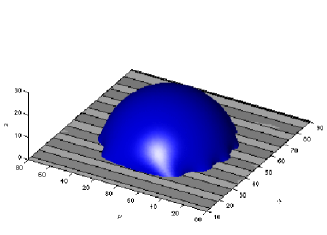
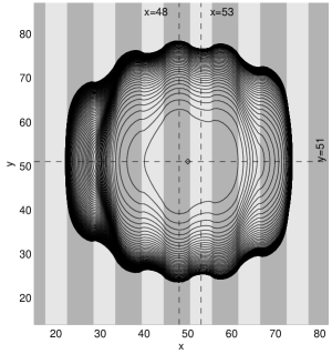
(c)
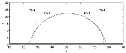
(d)

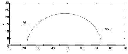
Figure 4: Spreading of an initially spherical droplet on a heterogeneous surface formed by alternating hydrophilic ($\theta_{phi}=50^{\circ}$, dark grey) and hydrophobic ($\theta_{pho}=110^{\circ}$, light grey) stripes of width equal to $6$ and $5$ respectively. A $99\times 99\times 60$ lattice and a droplet with an initial radius $R_{0}=19$ are used. The droplet initially just touches the substrate at $x=50$, $y=51$. $\tau=1.0$ and $\kappa=0.003$. Equilibrium is reached after $100~{}000$ iterations. (a) Three-dimensional view of the droplet at equilibrium. (b) Time evolution of the contact line. Each contour corresponds to $1000$ iterations. (c) Cross section at $x=48$ (solid) and $x=53$ (dashed) of the droplet profile at equilibrium. (d) Cross section at $y=51$ of the droplet profile at equilibrium.

5 Conclusion

We have used a three-dimensional lattice Boltzmann algorithm to model the spreading of a mesoscopic droplet. By incorporating the Cahn theory of wetting into the simulation we obtain a way of easily tuning the contact angle of the droplet on the substrate. This gives us the ability to simulate spreading on both homogeneous and heterogeneous surfaces.

The approach provides a well-controlled way of investigating the dependence of the spreading on such properties as the droplet volume, contact angles and the substrate geometry. Further work is in progress to systematically determine how these parameters affect the velocity and shapes of the spreading droplets. It would also be interesting to investigate the effect of physical inhomogeneities on the spreading and to consider a droplet spreading on a porous surface.

A particular aim of the work will be to compare the results to forthcoming experiments on substrates which have chemical patterning on mesoscopic length scale. This will allow increased understanding of both the experimental results and the model assumptions. For example we assume, as is the standard practice, no-slip boundary conditions on the velocity. These may not be appropriate on short length scales near a contact line. Moreover the liquid-gas density difference in lattice Boltzmann models is very small compared to real fluids and it is important to undertake further work to assess the effect of this on the modelling results.

References

- [1] P.G. de Gennes. Wetting: statics and dynamics. Review of Modern Physics, 57(3):827–863, 1985.
- [2] S. Succi. The Lattice Boltzmann Equation, For Fluid Dynamics and Beyond. Oxford University Press, 2001.
- [3] M.R. Swift, E. Orlandini, W.R. Osborn, and J.M. Yeomans. Lattice Boltzmann simulations of liquid-gas and binary fluid systems. Phys. Rev. E, 54:5051–5052, 1996.
- [4] X. Shan and H. Chen. Lattice Boltzmann models for simulating flows with multiple phases and components. Phys. Rev. E, 47:1815–1819, 1993.
- [5] X. He, S. Chen, and G.D. Doolen. A novel thermal model for the lattice Boltzmann method in incompressible limit. Journal of Computational Physics, 146:282–300, 1998.
- [6] F. Higuera S. Succi, E. Foti. 3-dimensional flows in complex geometries with the lattice Boltzmann method. EuroPhysics Letters, 10(5):433–438, 1989.
- [7] V.M. Kendon, J.C. Desplat, P. Bladon, and M.E. Cates. 3d spinodal decomposition in the inertial regime. Physical Review Letters, 83(3):576–579, 1999.
- [8] A. Dupuis and B. Chopard. Lattice gas modeling of scour formation under submarine pipelines. Journal of Computational Physics, 178(1):161–174, 2002.
- [9] D. Holdych, D.Rovas, J. Georgiadis, and R. Buckius. An improved hydrodynamics formulation for multiphase flow lattice Boltzmann models. Int. J. Mod. Phys. C, 9:1393–1404, 1998.
- [10] P. Raiskinmäki, A. Koponen, J. Merikoski, and J. Timonen. Spreading dynamics of three-dimensional droplets by the lattice-Boltzmann method. Computational Materials Science, 18:7–12, 2000.
- [11] A. Dupuis. From a lattice Boltzmann model to a parallel and reusable implementation of a virtual river. PhD thesis, University of Geneva, June 2002. http://cui.unige.ch/spc/PhDs/aDupuisPhD/phd.html.
- [12] C.M. Pooley. Private communication. 2003.
- [13] J.S. Rowlinson and B. Widom. Molecular theory of capillarity. Oxford: Clarendon, 1982.
- [14] J.W. Cahn. Critical point wetting. J. Chem. Phys., 66:3667–3672, 1977.
- [15] A.J. Briant, P. Papatzacos, and J.M. Yeomans. Lattice Boltzmann simulations of contact line motion in a liquid-gas system. Phil. Trans. R. Soc. Lond. A, 360:485–495, 2002.
- [16] T. Young. An essay on the cohesion of fluids. Phil. Trans. R. Soc. Lond., 95:65–87, 1805.
- [17] A. Marmur. Equilibrium and spreading of liquids on solid surfaces. Advances in Colloid and Interface Science, 19:75–102, 1983.
- [18] A. Zosel. Studies of the wetting kinetics of liquid drops on solid surfaces. Colloid Polym. Sci., 271:680–687, 1993.
- [19] J. Drelich, J. Miller, A. Kumar, and G. Whitesides. Wetting characteristics of liquid drops at heterogeneous surfaces. Colloid Surf. A, 93:1–13, 1994.
- [20] T. Pompe, A. Fery, and S. Herminghaus. Imaging liquid structures on inhomogeneous surfaces by scanning force microscopy. Langmuir, 14(10):2585–2588, 1998.
- [21] A. Cassie. Discuss. Faraday Soc., 3:11, 1948.