Directed geometrical worm algorithm applied to the quantum rotor model

Abstract

We discuss the implementation of a directed geometrical worm algorithm for the study of quantum link-current models. In this algorithm Monte Carlo updates are made through the biased reptation of a worm through the lattice. A directed algorithm is an algorithm where, during the construction of the worm, the probability for erasing the immediately preceding part of the worm, when adding a new part, is minimal. We introduce a simple numerical procedure for minimizing this probability. The procedure only depends on appropriately defined local probabilities and should be generally applicable. Furthermore we show how correlation functions, $C({\bf r},{\bf\tau})$ can be straightforwardly obtained from the probability of a worm to reach a site $({\bf r},{\bf\tau})$ away from its starting point independent of whether or not a directed version of the algorithm is used. Detailed analytical proofs of the validity of the Monte Carlo algorithms are presented for both the directed and un-directed geometrical worm algorithms. Results for auto-correlation times and Green functions are presented for the quantum rotor model.

I Introduction

Improving and developing new numerical algorithms lies at the heart of computational physics. Amongst others, Monte Carlo (MC) methods are often seen as the best choice for the study of phase transitions taking place in classical or quantum models. For the study of spin models for example, cluster algorithms, either in the classical Swendsen ; Wolff or quantum Evertz ; Sandvik ; Prokofev case, perform non-local moves in phase space, allowing for the treatment of systems much larger than with traditional local update methods (single spin-flip algorithms). These types of algorithms have almost completely solved the problem of critical slowing down arising near phase transitions.

The class of systems for which cluster methods are known to exist is limited, and it is therefore of great interest to search for new algorithms possessing the same efficient features for other models. In this context, we have proposed recently a non-local ”worm” algorithm for the study of quantum link-current models Alet03 . These models arise from a phase approximation of bosonic Hubbard models, but are also relevant in the context of quantum electrodynamics Banks . Previous MC simulations of the quantum link-current (quantum rotor) model used a local algorithm suffering from critical slowing down. In the new algorithm Alet03 updates are made by reptating a ”worm” through the lattice Prokofev ; Prokofev.Classical . Since the movement of the worm only depends on a few probabilities determined locally with respect to the current position of the “head” of the worm, we call this type of algorithm a geometrical worm algorithm as opposed to other recently developed worm algorithms based on high-temperature series expansions Prokofev.Classical . The geometrical worm algorithm gives rise to very small autocorrelation times and by directing the algorithm these autocorrelation times can be even further reduced.

In this paper, we briefly recall the principles of the geometrical worm algorithm Alet03 . During the construction of a worm a new part is added to the worm by moving the worm through one of the $\sigma$ nearest neighbor links. Usually the associated $\sigma$ probabilities, $p_{\sigma}$, are chosen in an un-biased geometrical way and there is therefore a significant probability that the new part of the worm will back-track in its own path, thereby erasing the immediately preceding part. In many cases this back-tracking (or bounce) probability is the dominant probability among the $\sigma$ probabilities and using these un-biased probabilities is therefore clearly rather wasteful. Here we describe an improvement of this geometric worm algorithm, which we call the directed worm algorithm, as a reference to recently developed directed loop methods for Quantum Monte Carlo simulations of spin systems Sylju . This directed geometrical worm algorithm is identical to its un-directed counterpart except for the fact that the probabilities $p_{\sigma}$ are now chosen in a biased way, using knowledge of the immediately preceding step in the construction of the worm. These biased probabilities can all be tabulated at the start of the simulation and the additional computational effort stems solely from the significantly wider distribution of the directed worms. The directed algorithm gives rise to even better results, as will be shown in the following part of this paper, where we present results on autocorrelation times for both directed and “undirected” worm algorithms. The procedure for choosing the “biased” probabilities leading to the directed algorithm is quite general and should be applicable to other algorithms that depend on local probabilities. Furthermore, we show how Green functions $C({\bf r},\tau)$ of the original quantum model can be measured efficiently during the construction of the worm by calculating the probability that the worm reaches a given site $({\bf r},\tau)$ away from its starting point, independently of whether a directed or un-directed algorithm is used. For both the derivation of the directed algorithm and the measurements of correlation functions, analytical proofs of the validity of the algorithms are presented.

The outline of the paper is as follows: in the next section, we present the quantum rotor model and introduce some useful notation. Then, a brief description of the ”undirected” worm algorithm is given in section III.1, before proceeding to the main contents of this paper, a description of the directed geometrical worm algorithm (section III.2). A simple procedure for numerically determining the biased probabilities for the worm moves is presented. In addition, we derive a proof of detailed balance for the directed worm algorithm. In order to compare our algorithms to related ones, we present in section III.3 another recent approach due to Prokof’ev and Svistunov Prokofev.Classical , originally based on high temperature series expansion for classical statistical models, which we therefore will refer to as ”classical worms” throughout this paper. In section IV, we estimate the efficiency of the algorithms by calculating auto-correlation times in the MC simulation, and compare to both undirected and classical algorithms. We then discuss the measurements of correlation functions within the worm algorithm in section V and show some results at a specific point of the phase diagram. We conclude with a discussion of the features of the directed algorithm.

II The model

Many magnetic systems, Josephson Junction arrays and several other systems can be described by a quantum rotor model Sachdev :

$$H_{\text{qr}}=\frac{U}{2}\sum_{\bf r}\left(\frac{1}{i}\frac{\partial}{\partial\theta_{\bf r}}\right)^{2}+i\sum_{\bf r}\mu_{\bf r}\frac{\partial}{\partial\theta_{\bf r}}-t\sum_{\langle{\bf r},{\bf r^{\prime}}\rangle}\cos(\theta_{\bf r}-\theta_{\bf r^{\prime}}).$$ (1)

Here, $\theta_{\bf r}$ is the phase of the quantum rotor, $t$ the renormalized coupling strength and $\mu_{\bf r}$ an effective chemical potential. If $\mu\equiv 0$ it can be shown that this model displays the same critical behavior as the $D+1$ dimensional $XY$-model. However, when $\mu_{\bf r}\neq 0$ this model is not amenable to direct numerical treatment in this representation due to the resulting imaginary term. It is therefore very noteworthy that an equivalent completely real representation in terms of link-currents exists even for non-zero $\mu_{\bf r}$. This link-current (Villain) representation is a classical (2+1)D equivalent Hamiltonian that is usually written in the following manner Sorensen :

$$H=\frac{1}{K}{\sum_{({\bf r},\tau)}}\left[\frac{1}{2}{\bf J}_{({\bf r},\tau)}^{2}-\mu_{\bf r}J_{({\bf r},\tau)}^{\tau}\right].$$ (2)

The sum is taken over all divergenceless current configurations ${\bf\nabla\cdot J}=0$. The degrees of freedom are “currents” ${\bf J}=(J^{x},J^{y},J^{\tau})$ living on the links of the lattice. These link variables $J^{x},J^{y},J^{\tau}=0,\pm 1,\pm 2,\pm 3\ldots$ are integers. $K$ is the effective temperature, varying like $t/U$ in the quantum rotor model. We refer to Ref. Sorensen for a precise derivation of this model and for a description of its physical implications.

Another incentive for studying the critical behavior of the quantum rotor model comes from the close relation between this model and bosonic systems. Bosonic systems with strong correlations are often described in terms of the (disordered) boson Hubbard model: $H_{\rm bH}=\sum_{\bf r}\left(\frac{U}{2}\hat{n}_{\bf r}^{2}-\mu_{\bf r}\hat{n}_{\bf r}\right)-t_{0}\sum_{\langle{\bf r},{\bf r^{\prime}}\rangle}(\hat{\Phi}^{\dagger}_{\bf r}\hat{\Phi}_{\bf r^{\prime}}+c.c)\ .$ The correlations are here described by $U$ the on-site repulsion. The hopping strength is given by $t_{0}$ and $\mu_{\bf r}$ the chemical potential varying uniformly in space between $\mu\pm\Delta$. $\hat{n}_{\bf r}=\hat{\Phi}^{\dagger}_{\bf r}\hat{\Phi}_{\bf r}$ is the number operator. If we set $\hat{\Phi}_{\bf r}\equiv|\hat{\Phi}_{\bf r}|e^{i\hat{\theta}_{\bf r}}$ and integrate out amplitude fluctuations, it can be shown that $H_{\rm bH}$ is equivalent to the quantum rotor model Sorensen . For systems where amplitude fluctuations can be neglected at the critical point, such as granular superconductors and Josephson junctions arrays, the quantum rotor model should therefore correctly describe the underlying quantum critical phenomena.

In the following we only discuss the quantum rotor model in $d=2$ dimensions corresponding to the $d+1$ dimensional link-current model. In general a non-zero $\mu$ will introduce separate dynamics for the time and space directions from which a dynamical critical exponent, $z$ can be defined. If the divergence of the spatial correlation length close to criticality is characterized by the exponent $\nu$, $z$ is defined by requiring that the correlation length in the time direction diverges with the exponent $z\nu$. For what we will be discussing here $\mu=0$ and $z=1$.

III Algorithms

III.1 The Geometrical (Undirected) Worm algorithm

The quantum rotor model has been extensively studied in the link-current representation using conventional Monte Carlo technique using local updates Sorensen ; Cha ; vanOtterlo ; Kisker ; Park .

Conventional Monte Carlo updates on the model (2) consists of updating simultaneously four link variables as shown in the left part of Fig. 1 (A). To ensure ergodicity, one also has to use global moves, updating a whole line of link variables (B in Fig. 1). The acceptance ratio for these global moves becomes exponentially small with the system size for large systems. Many interesting quantities such as the stiffness, necessary for the determination of the critical point, and current-current correlations, necessary for the calculation of transport properties such as the resistivity and the compressibility, are only non-zero when these global moves are successful. An effective Monte Carlo sampling of these global moves is therefore imperative and it is easy to understand that the performance of the local algorithm is rather poor, especially near a phase transition: critical slowing down in the Monte Carlo simulations prohibits the study of large system sizes.

In order to be able to correctly describe the directed geometrical worm algorithm we have to review the geometrical worm-cluster algorithm introduced in reference Alet03 in some detail. This algorithm allows for non-local moves as the ones depicted on the right part of Fig. 1 (C). The performances of this algorithm have been reported in the previous work Alet03 . This algorithm is closely related to other cluster algorithms Swendsen ; Wolff ; Evertz and especially to ”worm” algorithms Prokofev ; Sandvik ; Prokofev.Classical , from which we have borrowed the name. We stress that this algorithm is different from the ”classical” worm algorithm presented in Ref. Prokofev.Classical in the sense that it is geometrical: link variables are not “flipped” with a thermodynamic probability, instead, a new part of the worm is added by selecting a direction according to $\sigma$ locally determined probabilities $p_{\sigma}$. Since these probabilities only depend on the local environment we call them “geometrical” probabilities. Secondly, even though the local probabilities $p_{\sigma}$ do depend on the effective temperature, $K$, we always have $\sum_{\sigma}p_{\sigma}=1$ (per definition) and the only effect of the temperature is therefore to preferentially move the worm in one direction as opposed to another one. In some sense this is very similar to the N-fold way Bortz of performing Monte Carlo simulations.

Figure 1: Monte Carlo moves in the model. To ensure the divergenceless condition, only closed moves can be performed. On the left part of the figures, previous Monte Carlo updates with the local algorithm are depicted. On the right part is given an example of a move with the worm algorithm starting from an initial random site (black dot).

We now describe the contents of the geometrical algorithm: we update the configurations by moving a “worm” through the lattice of links. The links through which the worm pass are updated during its construction. The configurations generated during the construction (“reptation”) of the worm are not valid (the divergenceless of ${\bf J}$ is not fulfilled) but at the end of its path, when the worm forms a closed loop, this condition is verified and the final configuration is valid.

We first define a convention for the orientation of the lattice. Around each site with coordinates $({\bf r}=(x,y),\tau)$, there are six links on which the integer currents $J^{\sigma}_{({\bf r},\tau)}$ are defined with $\sigma=x,y,\tau,-x,-y,-\tau$. The change in $J^{\sigma}_{({\bf r},\tau)}$ that the worm will perform during its course depends on whether $\sigma$ is an incoming or outgoing link: here our convention is to consider positive $x,y,\tau$ as outgoing directions and $-x,-y,-\tau$ as incoming (see left lower part of Fig. 1).

If the worm is leaving the site $({\bf r},\tau)$ passing through an outgoing link $\sigma=x,y,\tau$, then

$$J^{\sigma}_{({\bf r},\tau)}\rightarrow J^{\sigma}_{({\bf r},\tau)}+1.$$ (3)

If it is leaving through an incoming link $\sigma=-x,-y,-\tau$ , we have

$$J^{\sigma}_{({\bf r},\tau)}\rightarrow J^{\sigma}_{({\bf r},\tau)}-1.$$ (4)

Graphically, the convention means that the update in $J^{\sigma}_{({\bf r},\tau)}$ is $+1$ ($-1$) if the worm goes in the same (opposite) direction as the arrows denoted in the left lower part of figure 1.

The construction (”reptation”) of the worm can be described the following way: first, we start the worm at a random site $N_{1}=({\bf r}_{1},\tau_{1})$ of the lattice (black dot in figure 1). From this site, the worm has the possibility to go to one of its six neighboring sites. To choose which direction to take, a weight $A^{\sigma}$ is calculated for the six directions $\sigma=\pm x,\pm y,\pm\tau$. For $A^{\sigma}$, we use a Metropolis-like weight:

$$A^{\sigma}=\min(1,\exp(-(E^{\prime}_{\sigma}-E_{\sigma})/K))$$ (5)

where $E_{\sigma}=\frac{1}{2}(J^{\sigma})^{2}-\mu J^{\sigma}\delta_{\sigma,\rm\tau}$ is the local energy carried by the link $\sigma$ and $E^{\prime}_{\sigma}=\frac{1}{2}(J^{\sigma}\pm 1)^{2}-\mu(J^{\sigma}\pm 1)\delta_{\sigma,\rm\tau}$ is the local energy on the link $\sigma$ if the worm passes through this link. The plus or minus sign depends on the incoming or outcoming nature of the link (see above). Please note that there are other possible choices for $A_{\sigma}$ AletPhD .

Once the $A_{\sigma}$’s are calculated, one computes the probabilities $p_{\sigma}$ by normalizing the weights $A_{\sigma}$ :

$$p_{\sigma}=\frac{A_{\sigma}}{N}$$ (6)

where $N=\sum_{\sigma}A_{\sigma}$ is the normalization. A random number uniformly distributed in $[0,1]$ is generated and a direction $\sigma$ chosen according to equation (6). Once a direction is chosen, the corresponding link variable $J^{\sigma}$ is updated by $\pm 1$ and the worm moved to the next lattice site in this direction.

From there, we apply the same procedure to choose another site, modify the link variable, move the worm until the worm eventually reaches its starting point and forms a closed loop. This is then the end of this non-local move.

To satisfy the detailed balance condition, this worm move must either be accepted or rejected. To check this, one has to store the initial and final normalizations $N_{s_{1}}^{i}$ and $N_{s_{1}}^{f}$ (calculated as in Eq. 6) of the weights at the site $s_{1}=({\bf r}_{1},\tau_{1})$. $N_{s_{1}}^{i}$ is the initial normalization before the worm is inserted and $N_{s_{1}}^{f}$ the final normalization after the worm reaches the initial point. The worm move is then accepted with probability $N_{s_{1}}^{i}/N_{s_{1}}^{f}$. If the move is rejected, we have to cancel all changes of the link-currents made during the construction of the worm. During a typical simulation the rejection probability is usually very small.

As already mentioned, the link configurations generated during the worm move do not satisfy the divergenceless constraint, but it is easy to see that the final configuration does. It is important to note that the worm may pass many times though the same link and that at each step, it can bounce back (back-track) to the previous lattice site in its path.

A proof of detailed balance for this algorithm is obtained by considering the moves of the worm and of an anti-worm, going exactly in the opposite direction Alet03 . This worm algorithm satisfies ergodicity since the worm can make local loops and line moves as in the local algorithm, which is ergodic.

All in all, the geometrical un-directed worm algorithm can be summarized using the following pseudo-algorithm:

1. Choose a random initial site $s_{1}=({\bf r}_{1},\tau_{1})$ in the space-time lattice.

2. For each of the directions $\sigma=\pm x,\pm y,\pm\tau$, calculate the weights $A^{\sigma}_{s_{i}}$ with $A^{\sigma}_{s_{i}}=$ $\min(1,\exp(-\Delta E_{s_{i}}^{\sigma}/K)),$ $\Delta E_{s_{i}}^{\sigma}=E^{\prime\sigma}_{s_{i}}-E_{s_{i}}^{\sigma}.$

3. Calculate the normalization $N_{s_{i}}=\sum_{\sigma}A^{\sigma}_{s_{i}}$ and the associated probabilities $p^{\sigma}_{s_{i}}={A^{\sigma}_{s_{i}}}/{N_{s_{i}}}.$

4. According to the probabilities, $p^{\sigma}_{s_{i}}$, choose a direction $\sigma$.

5. Update the $J^{\sigma}_{s_{i}}$ for the direction chosen and move the worm to the new lattice site $s_{i+1}$.

6. If $s_{i}\neq s_{1}$ goto 2.

7. Calculate the normalizations $\bar{N}_{s_{1}}$ and $N_{s_{1}}$ of the initial site, $s_{1}$, with and without the worm present. Erase the worm with probability $P^{e}=1-\min(1,N_{s_{1}}/{\bar{N}_{s_{1}}})$.

III.2 The Directed Geometrical Worm algorithm

The above algorithm for geometrical worms is not optimal since the worm quite often will choose to erase itself by returning to the previous site. While it is in general not possible to always set this back-tracking (or bounce) probability to zero it is quite straightforward to choose the probabilities $p^{\sigma}_{s_{i}}$ such that the bounce or back-tracking probability will be eliminated in almost all cases and in general will be as small as possible. The procedure for doing this amounts to solving a simple linear programming optimizing problem. If we consider models with disorder this has to be done at each site, but the correctly optimized (biased) probabilities $p^{\sigma}_{s_{i}}$ can still be tabulated at the start of the calculation.

In order to see how we can minimize the back-tracking probability let us define the $6\times 6$ matrix $P_{s_{i}}$ of probabilities where the element $P_{s_{i}}^{kl}$ of the matrix $P_{s_{i}}$ is given by the conditional probability $p_{s_{i}}(\sigma_{k}|\sigma_{l})$ for going in the direction $\sigma_{k}$ at the site $s_{i}$ if the worm is coming from the direction $\sigma_{l}$. The back-tracking probabilities at the site $s_{i}$ now correspond to the diagonal elements of the matrix $P_{s_{i}}$. For the algorithm described in the previous section $p_{s_{i}}(\sigma_{k}|\sigma_{l})$ was simply chosen as $A^{\sigma_{k}}_{s_{i}}/{N_{s_{i}}}$ independent of $\sigma_{l}$. Thus all the columns of $P_{s_{i}}$ were the same and $P_{s_{i}}$ had in general rather large diagonal elements. However, as we shall see below, the matrix $P_{s_{i}}$ only needs to satisfy the following two conditions in order to define a working geometrical worm algorithm. These conditions are:

$$\sum_{k}p_{s_{i}}(\sigma_{k}|\sigma_{l}) = 1\ \ {(\rm probability)}$$ (7)

$$\frac{P_{s_{i}}^{kl}}{P_{s_{i}}^{lk}}\equiv\frac{p_{s_{i}}(\sigma_{k}|\sigma_{l})}{p_{s_{i}}(\sigma_{l}|\sigma_{k})} = \frac{A^{\sigma_{k}}_{s_{i}}}{A^{\sigma_{l}}_{s_{i}}}\ \ {(\rm detailed\ balance)}.$$ (8)

These conditions are not very restrictive and will in most cases allow us to define a matrix $P_{s_{i}}$ with all the diagonal elements (back-tracking probabilities) equal to zero. The conventional geometrical worm algorithm, discussed in the previous section, corresponds to $P_{s_{i}}^{kl}=A^{\sigma_{k}}_{s_{i}}/{N_{s_{i}}}$.

If we define a function $f$ as the sum of the diagonal elements of $P_{s_{i}}$, $f=\sum_{k}P_{s_{i}}^{kk}$, we can reformulate the search for a matrix $P_{s_{i}}$ with minimal diagonal elements as a standard linear programming problem. Writing $P_{s_{i}}^{kk}=1-\sum_{l\neq k}P_{s_{i}}^{kl}$ we should minimize $f$ subject to the constraints $\sum_{l\neq k}P_{s_{i}}^{kl}\leq 1\ \ \forall k$. The minimum can be found using standard techniques of linear programming numrec and corresponds in almost all cases to $f=0$. The matrix $P_{s_{i}}$ depends on the value of all the 6 link-currents $J^{\sigma}_{s_{i}}$. During the construction of the worm only sites where $J_{s_{i}}^{-x}+J_{s_{i}}^{-y}+J_{s_{i}}^{-\tau}-J_{s_{i}}^{x}-J_{s_{i}}^{y}-J_{s_{i}}^{\tau}=1$, $s_{i}\neq s_{1}$ occur. Since in general $|J^{\sigma}_{s_{i}}|$ will almost never exceed a certain value $J_{\rm max}$ it is easy to construct a lookup table for the matrices $P_{s_{i}}$ at the beginning of the simulation and only calculate $P_{s_{i}}(\{J^{\sigma}_{s_{i}}\})$ during the simulation if for some $\sigma$ $|J^{\sigma}_{s_{i}}|>J_{\rm max}$.

This idea of minimizing the bounce processes is also at the heart of Quantum Monte Carlo directed loop methods Sylju . The previous restrictions on the matrix $P$ and the way to solve them numerically are indeed very general, and constitute a simple framework for how one can construct a directed algorithm out of a ”standard” non-local loop, worm or cluster algorithm.

We can now define a directed geometrical worm algorithm with minimal back-tracking probability. Using a pseudo-code notation we have:

1. Choose a random initial site $s_{1}=({\bf r}_{1},\tau_{1})$ in the space-time lattice.

2. If $i=1$ then: For each of the directions $\sigma=\pm x,\pm y,\pm\tau$, calculate the weights $A^{\sigma}_{s_{i}}$ with $A^{\sigma}_{s_{i}}=\min(1,\exp(-\Delta E_{s_{i}}^{\sigma}/K)),$ $\Delta E_{s_{i}}^{\sigma}=E^{\prime\sigma}_{s_{i}}-E_{s_{i}}^{\sigma}$. Calculate the normalization $N_{s_{i}}=\sum_{\sigma}A^{\sigma}_{s_{i}}$ and the associated probabilities $p^{\sigma}_{s_{i}}={A^{\sigma}_{s_{i}}}/{N_{s_{i}}}.$ Else: According to the incoming direction, $\sigma_{l}$, set $p^{\sigma}_{s_{i}}$ equal to the $l$’th column of $P_{s_{i}}$.

3. According to the probabilities, $p^{\sigma}_{s_{i}}$, choose a direction $\sigma$.

4. Update $J^{\sigma}_{s_{i}}$ for the direction chosen and move the worm to the new lattice site $s_{i+1}$.

5. If $s_{i}\neq s_{1}$ goto 2.

6. Calculate the normalizations $\bar{N}_{s_{1}}$, of the site $s_{1}$ with the worm present, and $N_{s_{1}}$, without the worm. Erase the worm with probability $P^{e}=1-\min(1,N_{s_{1}}$/$\bar{N}_{s_{1}}$).

Now we turn to the proof of detailed balance for the directed algorithm. Let us consider the case where the worm, $w$, visits the sites $\{s_{1}\ldots s_{N}\}$ where $s_{1}$ is the initial site. The worm then goes through the corresponding link variables $\{l_{1}\ldots l_{N}\}$, with $l_{i}$ connecting $s_{i}$ and $s_{i+1}$. Note that $s_{N}$ is the last site visited before the worm reaches $s_{1}$. Hence, $s_{N}$ and $s_{1}$ are connected by the link $l_{N}$. The total probability for constructing the worm $w$ is then given by:

$$P_{w}=P_{s_{1}}(1-P_{w}^{e})\frac{A_{s_{1}}^{\sigma}}{{N_{s_{1}}}}\prod_{i=2}^{N}p_{s_{i}}(s_{i+1}|s_{i-1}).$$ (9)

The index $\sigma$ denotes the direction needed to go from $s_{1}$ to $s_{2}$, $P_{s_{1}}$ is the probability for choosing site $s_{1}$ as the starting point and $P_{w}^{e}$ is the probability for erasing the worm $w$ after construction. $p_{s_{i}}(s_{i+1}|s_{i-1})$ is the conditional probability for continuing to site $s_{i+1}$, at site $s_{i}$, given that the worm is coming from $s_{i-1}$. If the worm $w$ has been accepted we have to consider the probability for reversing the move. That is, we consider the probability for constructing an anti-worm $\bar{w}$ annihilating the worm $w$. We have:

$$P_{\bar{w}}=P_{\bar{s}_{1}}(1-P_{\bar{w}}^{e})\frac{{\bar{A}}_{s_{1}}^{\bar{\sigma}}}{{\bar{N}}_{\bar{s}_{1}}}\prod_{i=N}^{2}p_{s_{i}}(s_{i-1}|s_{i+1}).$$ (10)

Here, the index $\sigma$ denotes the direction needed to go from $s_{1}$ to $s_{N}$, Note that, in this case the sites are visited in the opposite order, $s_{1},s_{N},\ldots,s_{2}$. From Eq. (8) we have that $p_{s_{i}}(s_{i+1}|s_{i-1})/p_{s_{i}}(s_{i-1}|s_{i+1})=A^{\sigma_{k}}_{s_{i}}/{\bar{A}^{\sigma_{l}}_{s_{i}}}$. Since,

$${A_{s_{i}}^{\sigma}}/{\bar{A}_{s_{i}}^{\sigma}}=\exp(-\Delta E_{s_{i}}^{\sigma}/K),\ i=1\ldots N,$$ (11)

and since $P_{s_{1}}=P_{\bar{s}_{1}}$, we find:

$$\frac{P_{w}}{P_{\bar{w}}}=\frac{1-P_{w}^{e}}{1-P_{\bar{w}}^{e}}\frac{\bar{N}_{\bar{s}_{1}}}{N_{s_{1}}}\exp(-\Delta E_{\rm Tot}/K).$$ (12)

where $\Delta E_{\rm Tot}$ is the total energy difference between a configuration with and without the worm $w$ present. With our definition of $P^{e}$ we see that $(1-P^{e}(w))/(1-P^{e}(\bar{w}))=N_{s_{1}}/{\bar{N}_{s_{1}}}$ and it follows that:

$$\frac{P_{w}}{P_{\bar{w}}}=\exp(-\Delta E_{\rm Tot}/K).$$ (13)

For a worm of length $N$ there are $N$ starting sites that will yield the same final configuration. The above proof shows that for each of the starting sites there exists an anti-worm, $\bar{w}$, such that $P_{w}=\exp(-\Delta E_{\rm Tot}/K)P_{\bar{w}}$. Hence, if we by $\mu$ denote the configuration without the worm and $\nu$ the configuration with the worm and furthermore let $P_{w}(s_{i})$ denote the probability of building the worm $w$ starting from site $s_{i}$, we see that:

$$\frac{P(\mu\to\nu)}{P(\nu\to\mu)} =\frac{\sum_{i}^{N}P_{w}(s_{i})}{\sum_{i}^{N}P_{\bar{w}}(s_{i})}$$ (14)

$$=\frac{\sum_{i}^{N}P_{\bar{w}}(s_{i})}{\sum_{i}^{N}P_{\bar{w}}(s_{i})}\exp(-\Delta E_{\rm Tot}/K)$$

$$=\exp(-\Delta E_{\rm Tot}/K).$$

Ergodicity is proved the same way as for the undirected algorithm as the worm can perform local loops and wind around the lattice in any direction, as in the conventional algorithm.

III.3 The Classical Worm algorithm

Prokof’ev and Svistunov Prokofev.Classical have proposed a very elegant way of performing Monte Carlo simulations on the high temperature expansion of classical statistical mechanical models using worm algorithms. In order to distinguish between the algorithms we call this algorithm the classical worm algorithm. In a recent study Prokofev.QR these authors have performed simulations on the quantum rotor model in the link-current representation, Eq. (2). Due to the divergenceless constraint, the classical worm algorithm is in this case quite close to the geometrical worm algorithm proposed previously in Ref. Alet03, and not directly related to the high temperature expansion of this model. Recasting their algorithm in the same framework used above we outline our understanding of their algorithm below for comparison:

1. Choose a random initial site $s_{1}=({\bf r}_{1},\tau_{1})$ in the space-time lattice.

2. For each of the directions $\sigma=\pm x,\pm y,\pm\tau$, calculate the probabilities $A^{\sigma}_{s_{i}}$ with $A^{\sigma}_{s_{i}}=\min(1,\exp(-\Delta E_{s_{i}}^{\sigma}/K)),$ $\Delta E_{s_{i}}^{\sigma}=E^{\prime\sigma}_{s_{i}}-E_{s_{i}}^{\sigma}$.

3. With uniform probability choose a direction $\sigma$.

4. With probability $A^{\sigma}_{s_{i}}$ accept to go in the direction $\sigma$, and with probability $1-A^{\sigma}_{s_{i}}$ go to 3.

5. Update $J^{\sigma}_{s_{i}}$ for the direction chosen and move the worm to the new lattice site $s_{i+1}$.

6. If $s_{i}\neq s_{1}$ go to 2.

7. If $s_{i}=s_{1}$ go to 1 with probability $p_{0}$ and to 3 with probability $1-p_{0}$ ($p_{0}\in(0,1)$ and usually $p_{0}=1/2$). We use $p_{0}=1/2$ in the following.

One advantage of this algorithm is its simplicity and the fact that a constructed worm is always accepted, on the other hand this algorithm is not directed and steps 3-4 above are quite wasteful since in many cases the worm is not moved. This is avoided in the geometrical worm algorithm at the price of occasionally having to reject a complete worm. The geometrical worm algorithm, as described in the preceding sections, should be straightforwardly applicable to the high temperature expansion as it was done in Ref. Prokofev.Classical using the classical worm algorithm. We expect that this would enhance the efficiency of the Monte Carlo sampling.

IV Performance of the algorithms

Here we present results on autocorrelation times obtained with both directed and undirected algorithms. For the sake of brevity, we restrict ourselves to the case $\mu=0$, where the critical point is known with high precision, and where results on autocorrelations for the undirected worm algorithm have already been published Alet03 . All the results presented in this section correspond to runs on cubic lattices of $10^{7}$-$10^{8}$ Monte Carlo worms for a value of $K=0.333$, extremely close to the critical point (estimated as $K_{c}=0.33305(5)$ in Ref. Alet03 ). In principle, simulations should be performed on lattices of size $L\times L\times L_{\tau}$, but here since the dynamical exponent $z=1$ at $\mu=0$, we can set $L_{\tau}=L$. We focus here on calculations of the energy $E=\langle H\rangle$ and the stiffness $\rho$ defined as

$$\rho=\frac{1}{L^{3}}\langle(\sum_{{\bf r},\tau}J^{x}_{{\bf r},\tau})^{2}\rangle$$ (15)

where $L$ is the linear size of the lattice.

For the simulations with directed worms, we restrict ourselves to $|J|\leq 3$ for the tabulation of probabilities. Probabilities involving higher values of $|J|$ were calculated during the construction of the worm. Such configurations were found to be exceedingly rare.

For the case at hand, only $1\%$ of the ”scattering” matrices $P_{s_{i}}$ contained diagonal elements corresponding to a non-zero back-tracking probability. Moreover, these back-tracking (bounce) processes were found to occur for very unlikely configurations. The acceptance rate, $1-P^{e}$, is very high for both algorithms at $K_{c}$ (around $98\%$ for undirected worms and $97\%$ for directed worms for all lattice sizes). For the classical worms, all worms are accepted due to the nature of the algorithm. However, we found that many proposed attempts at changing one link were refused (more than $60\%$ in our simulations).

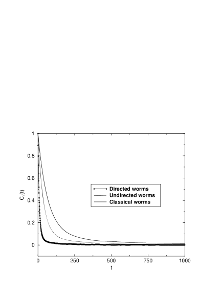
Figure 2: Auto-correlation function of stiffness versus Monte Carlo time (defined by one worm construction - see text -) for $L=56$ at $K=0.333$ for directed (circle), undirected (dotted line) and classical (solid line) algorithms.

In figure 2, we present the autocorrelation function of stiffness for a lattice size $L=56$, for directed, undirected and classical worms. The autocorrelation function $C_{\cal O}(t)$ of an observable ${\cal O}$ is defined in the standard way:

$$C_{\cal O}(t)=\frac{\langle{\cal O}(t){\cal O}(0)\rangle-\langle{\cal O}\rangle^{2}}{\langle{\cal O}^{2}{\rangle-\langle{\cal O}\rangle}^{2}}$$ (16)

where $\langle\ldots\rangle$ denotes statistical average and $t$ is the MC time, measured in the number of constructed worms (accepted or not). We clearly see in figure 2 that the directed worm algorithm is more efficient at decorrelating the data than undirected and classical worms, the latter having the longest autocorrelation times.

Now we define the autocorrelation time $\tau_{\cal O}$ of an observable $\cal O$. In Ref. Alet03 , $\tau_{\cal O}$ was defined as the greater time of a double-exponential fit of the autocorrelation function. Here we use a much simpler definition, independent of any fitting procedure: $\tau_{\cal O}$ is defined as the time where the normalized autocorrelation function decrease below a threshold $t_{\cal O}$. We can use different thresholds for different observables $\cal O$. Since for small lattices and especially for directed worms, autocorrelation times are small, and since $C_{\cal O}(t)$ is known only for discrete values of $t$, $\tau_{\cal O}$ is determined by a simple linear interpolation between the two times surrounding the threshold. It is important to note that the values of the autocorrelation time depends on the threshold $t_{\cal O}$, but the dependence on lattice size of these autocorrelation times should not change as long as $t_{\cal O}$ is small enough. Error bars on $t_{\cal O}$ have been estimated by slightly changing the threshold, by an amount in between $2\%$ and $5\%$ in this work.

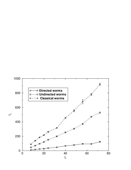
Figure 3: Auto-correlation times of the stiffness, $\rho$, for directed, undirected and classical algorithms versus lattice size L. Shown are the raw auto-correlations times, before rescaling to take into account the computational effort expended.

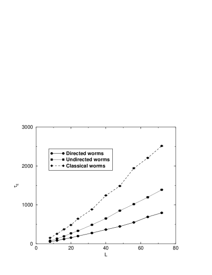
Figure 4: Auto-correlation times of energy $E$ for the three algorithms versus lattice size L. Shown are the raw auto-correlations times, before rescaling to take into account the corresponding computational effort expended.

Using the above mentioned determination of autocorrelation times, we extract autocorrelation times of the stiffness $\rho$ and the energy $E$ for directed, undirected and classical worms. The threshold was set the same for all algorithms when comparing the same quantity: we used through this work $t_{\rho}=0.02$ for the stiffness and $t_{E}=0.05$ for the energy. Scaling of these times with the lattice size is shown in figure 3 for stiffness and in figure 4 for energy. It can be seen that whereas autocorrelation times grow approximatively linearly with lattice size for all algorithms, the slope is significantly smaller for the directed worm algorithm.

It is clear from these results that the directed algorithm significantly reduces the autocorrelation times. However, the average size of the directed worms could be larger, and hence on average consume more computational time. For all algorithms the computational effort is linearly proportional to the length of the worm. To make an honest comparison, we therefore have to multiply the autocorrelation times by the number of attempted changes per link, which we define as $\langle w\rangle/(3L^{3})$, where $\langle w\rangle$ is the mean worm size (the mean number of links the worm has attempted to visit), $L$ the lattice size preceded by an irrelevant factor indicating that there are $3$ links per site. For the classical worms, the mean worm size $\langle w\rangle$ is defined as the total number of proposed attempts (step 4 in the pseudo-code presentation in section III.3). In order to make an un-biased comparison of the three algorithms it is here necessary to include the updates refused during the construction of the classical worms in the definition of $\langle w\rangle$.

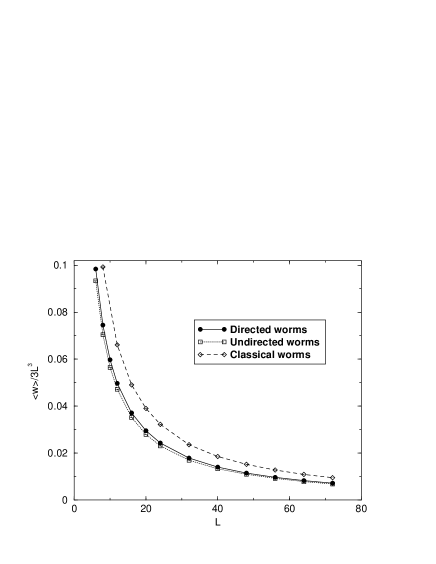
Figure 5: Mean size $\langle w\rangle$ divided by $3L^{3}$ versus lattice size $L$ for directed, undirected and classical worms.

As mentioned, the computational effort (the CPU time) is linear in $\langle w\rangle$ for all algorithms. An equivalent rescaling was used in Ref. Alet03 in order to make a fair comparison with the local algorithm. In Fig. 5 is shown the mean worm size $\langle w\rangle$ (divided by $3L^{3}$) for the three algorithms versus lattice size, corresponding to the average fraction of the total number of links occupied by the worm. In both cases, we see that this fraction decreases with $L$. We also note that the classical worms are longer than in the other proposed algorithms, which will result in larger autocorrelation times. Directed and undirected worms are almost of the same size, with very slightly larger directed worms. The corresponding effect on the value of rescaled effort (presented in the next paragraph) will be small when comparing autocorrelation times for those algorithms, however we wish to keep it present for a more fair analysis.

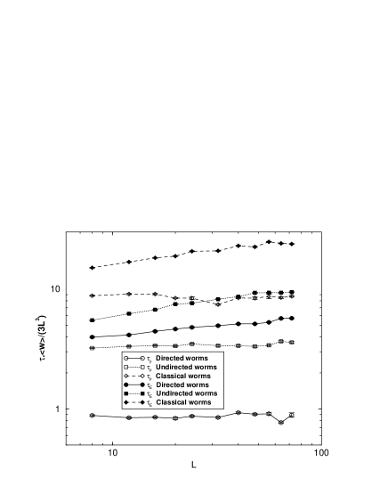
Figure 6: Auto-correlation times of stiffness $\rho$ and energy $E$ for the three presented algorithms versus lattice size L. These auto-correlations times are rescaled auto-correlation times where the computational effort is taken into account.

Having discussed the behavior of $\langle w\rangle$ we now take into account the computational effort used to construct the worm by rescaling the auto-correlation times by $\langle w\rangle/(3L^{3})$. We show in figure 6 the rescaled auto-correlation times for the three algorithms. We find that the auto-correlation times per link stay reasonably small for all algorithms, but the directed algorithm clearly gives better results, with auto-correlation times smaller by a factor around $4$ ($1.5-1.7$) for the stiffness (energy) with respect to the undirected algorithm, and a factor around $10$ ($4$) with respect to the classical worm for the largest sizes. The fact that both algorithms are more efficient at decorrelating the stiffness than the energy seems to indicate that the worms couple more effectively to “winding modes”, from which the stiffness is uniquely determined, than to simple local modes which determine the energy. With the same argument, we can see that directed worms are more efficient at updating winding modes than undirected or classical worms.

The actual distribution of the size of the worms generated, $P(w)$ is also of interest. In Fig. 7 we show results for the probability density, $P(w)$ for generating a worm occupying a fraction of $w/3L^{3}$ of the lattice, as a function of $w/3L^{3}$ for the directed and un-directed algorithms. The classical worm algorithm has a distribution identical to the one shown for the un-directed algorithm. Clearly, the directed worms have a somewhat broader distribution but for both algorithms the distribution follows a power-law form $P(w)\sim w^{-\alpha}$ with $\alpha\sim 1.37$. The power-law behavior is to be expected since the simulations were performed at the critical point. Away from the critical point we have verified that the initial power-law form crosses over to an exponential behavior at large arguments.

To summarize, we find that in all cases, rescaled auto-correlation times stay almost constant with the lattice size, but could also be fitted with a very small power-law or logarithm, showing an almost complete elimination of critical slowing down. All in all, the main result of this section is that directed worms produce less correlated data (smaller autocorrelation times), even if the scaling is good for all the three (directed, undirected and classical) algorithms. We also note that the geometrical worm algorithms perform better than the classical worm algorithm.

The fact that both directed and undirected algorithms have almost the same scaling of the rescaled autocorrelation time with $L$, seems also to be observed for the directed loop Quantum Monte Carlo cluster algorithms Sylju .

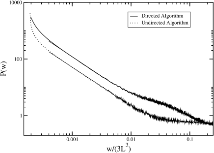
Figure 7: The probability density, $P(w)$ for generating a worm occupying a fraction of $w/3L^{3}$ of the lattice, as a function of $w/3L^{3}$ for the directed and un-directed algorithms. Shown are results for a lattice of linear size $L=56$ at $K=K_{c}$. The solid lines indicate power-law fits to the data.

V The Correlation Functions

V.1 Measurements of correlation functions with worm algorithms

For the quantum rotor model, the correlation functions of interest have the following form Sorensen :

$$C({\bf r,r^{\prime}},\tau,\tau^{\prime})=\langle e^{i(\hat{\theta}_{\bf r}(\tau)-\hat{\theta}_{\bf r^{\prime}}(\tau^{\prime}))}\rangle\ ,$$ (17)

where the $\hat{\theta}$’s are operators for the phase of the bosons, and $e^{i\hat{\theta}_{\bf r}(\tau)}=e^{\tau H}e^{i\hat{\theta}_{\bf r}}e^{-\tau H}$. Due to translational invariance, $C({\bf r,r^{\prime}},\tau,\tau^{\prime})=C({\bf r-r^{\prime}},\tau-\tau^{\prime})$. Physically this corresponds to creating a particle at $({\bf r},\tau)$ and destroying it at $({\bf r^{\prime}},\tau^{\prime})$. When this correlation function is mapped onto the link-current representation the creation and destruction of the particle is interpreted as a particle current going from $({\bf r},\tau)$ to $({\bf r^{\prime}},\tau^{\prime})$. As is evident from the definition of the correlation function in Eq. (17) the value of the correlation function can not depend on the specific path taken from $({\bf r},\tau)$ to $({\bf r^{\prime}},\tau^{\prime})$ as long as we take into account the fact that going in the $x,y,\tau$ increases the local current, whereas going in the $-x,-y,-\tau$ direction decreases the local current. In the link current representation this correlation function can be written Sorensen in the following way:

$$C({\bf r},\tau)=\langle\prod_{({\bf r}_{i},\tau_{i})\;\rm\in path}$$

$$\exp\left\{-\frac{1}{K}\left({\rm sign}(\sigma_{i})\left(J_{({\bf r}_{i},\tau_{i})}^{\nu}-\delta_{\sigma_{i},\pm\tau}\tilde{\mu}_{\bf r_{i}}\right)+\frac{1}{2}\right)\right\}\ \rangle,$$

(18)

where “path” is any path on the space-lattice connecting two points a distance $({\bf r},\tau)$ apart and $\sigma_{i}$ is the direction needed to go from $({\bf r_{i}},\tau_{i})$ to $({\bf r_{i+1}},\tau_{i+1})$, $\sigma_{i}=\pm x,\pm y,\pm\tau$. When going in the direction $\sigma_{i}=x,y,\tau$ we propagate a particle and the correlation function corresponds to incrementing the corresponding link-variable by one. When going in the direction $\sigma_{i}=-x,-y,-\tau$ we propagate a hole in the $x,y,z$ direction and the correlation function corresponds to decrementing the corresponding link-variable by one. This is indicated in the expression Eq. (18) by ${\rm sign}(\sigma_{i})$. Furthermore, we only get a contribution from $\mu_{\bf r_{i}}$ whenever we go in the $\tau-$direction and we take this into account by $\delta_{\sigma_{i},\pm\tau}$. If we define $J^{-x}_{(x,y,\tau)}=-J^{x}_{(x-1,y,\tau)}$ with analogous definitions for the other directions we see that by incrementing and decrementing the link-current variables in the above manor $\sum_{\sigma}J^{\sigma}_{({\bf r},\tau}=0$ at all the sites between $({\bf r_{i}},\tau_{i})$ and $({\bf r_{i+1}},\tau_{i+1})$. The current is divergenceless at all the intermediary sites. The sites $({\bf r_{i}},\tau_{i})$ and $({\bf r_{i+1}},\tau_{i+1})$ will have non-zero divergence with $\sum_{\sigma}J^{\sigma}_{({\bf r},\tau}=1$ corresponding to a site where a particle is created (or a hole destroyed). A site with $\sum_{\sigma}J^{\sigma}_{({\bf r},\tau}=-1$ is a site where a hole is created (or a particle destroyed). In Fig. 8 we show two possible paths ${\cal P}_{a}$ and ${\cal P}_{b}$ for the evaluation of the correlation function $C({\bf r},\tau)$.

Figure 8: Two possible paths, ${\cal P}_{a}$ and ${\cal P}_{b}$, for the evaluation of $C({\bf r},\tau)$. When the path is going in the $x,y,\tau$ direction a particle is propagated in the forward direction corresponding to an increment in the current. When the path is going in $-x,-y,-\tau$ direction we propagate a hole in the forward direction corresponding to a decrement in the current. The solid circles correspond to sites where a single particle is created or destroyed.

As usual, $C({\bf r},\tau)=C({\bf r}+L,\tau+L_{\tau})$ but $C({\bf r},\tau)$ is in general not equal to $C({\bf r},-\tau)$.

Previous work Sorensen ; Kisker have attempted to calculate the correlation function by evaluating the thermal expectation value in Eq. (18) along a straight path from $({\bf r},\tau)$ to $({\bf r^{\prime}},\tau^{\prime})$. Although formally correct, this method fails for large arguments of the correlation function due to the fact that for a given configuration of the link-variables roughly only one specific path between $({\bf r},\tau)$ and $({\bf r^{\prime}},\tau^{\prime})$ will yield a contribution of order 1.

The geometrical worm algorithm allows for a much more efficient way of evaluating the correlation functions. In essence, before the worm returns to the starting site, the path of the worm corresponds precisely to the creation of a particle at site $s_{1}$ and the destruction at the current site $s_{i}$ with a current going between the two sites. This is precisely the Greens function that we want to calculate. More precisely we extend Eq. (18) to include a summation over all possible paths:

$$C({\bf r},\tau)=\frac{1}{N_{\cal P}}\sum_{\cal P}\langle\prod_{({\bf r}_{i},\tau_{i})\;\rm\in{\cal P}}$$

$$\exp\left\{-\frac{1}{K}\left({\rm sign}(\sigma_{i})\left(J_{({\bf r}_{i},\tau_{i})}^{\nu}-\delta_{\sigma_{i},\pm\tau}\tilde{\mu}_{\bf r_{i}}\right)+\frac{1}{2}\right)\right\}\ \rangle.$$

(19)

Here ${\cal P}$ is a path for the correlation function and $N_{\cal P}$ is the number of paths included in the sum. Since the geometrical worm algorithm generates paths between $({\bf r},\tau)$ and $({\bf r}_{n},\tau_{n})$ with the correct exponential factor (except for a multiplicative constant) it is now easy to calculate the correlation functions.

Suppose that we, by using either the directed or undirected worm algorithm, have reached the equilibrium configuration $\mu$. The probability for, during the construction of a worm starting at site $s_{1}=({\bf r}_{1},\tau_{1})$, creating a current $j$ that reaches $s_{n}=({\bf r}_{n},\tau_{n})\neq s_{1}$ is given by:

$$P(j;\mu\to\mu^{\prime})=P(s_{1})\prod_{i=1}^{n-1}\frac{A_{s_{i}}^{\sigma}}{N_{s_{i}}}$$ (20)

for the undirected algorithm. For the directed algorithm we have:

$$P(j;\mu\to\mu^{\prime})=P(s_{1})\frac{A_{s_{1}}^{\sigma}}{N_{s_{1}}}\prod_{i=2}^{n-1}p_{s_{i}}(s_{i+1}|s_{i-1}).$$ (21)

If we call the resulting state $\mu^{\prime}$ we can calculate the probability for, starting from $\mu^{\prime}$, creating an anti-current, $\bar{j}$, going from $s_{n}$ to $s_{1}$. We find for the undirected algorithm:

$$P(\bar{j};\mu^{\prime}\to\mu)=P(s_{n})\prod_{i=n}^{2}\frac{\bar{A}_{s_{i}}^{\sigma}}{N_{s_{i}}},$$ (22)

and for the directed algorithm:

$$P(\bar{j};\mu^{\prime}\to\mu)=P(s_{N})\frac{\bar{A}_{s_{n}}^{\sigma}}{\bar{N}_{s_{n}}}\prod_{i=n-1}^{2}p_{s_{i}}(s_{i-1}|s_{i+1}).$$ (23)

In both cases we see that

$$\frac{P(j;\mu\to\mu^{\prime})}{P(\bar{j};\mu^{\prime}\to\mu)}=\frac{\bar{N}_{s_{n}}}{N_{s_{1}}}\prod_{({\bf r}_{i},\tau_{i})\;\rm\in{\cal P}}$$

$$\exp\left\{-\frac{1}{K}\left({\rm sign}(\sigma_{i})\left(J_{({\bf r}_{i},\tau_{i})}^{\nu}-\delta_{\sigma_{i},\pm\tau}\tilde{\mu}_{\bf r_{i}}\right)+\frac{1}{2}\right)\right\}.$$

Hence, we see that for both algorithms the intermediate states generated during the construction of the worm follows precisely the distribution needed apart from the factor ${\bar{N}}_{s_{n}}/{N_{s_{1}}}$. It follows that whenever a worm reaches a point a distance $({\bf r},\tau)$ away from the initial point it contributes a factor of $N_{s_{1}}/{\bar{N}_{s_{n}}}$ to the correlation function of argument $({\bf r},\tau)$. Note that it follows from the above proof that all worms, even the ones that are finally rejected, have to be included in the calculation of the Greens functions. Per definition $C(0,0,0)\equiv C(L,L,L_{\tau})\equiv 1$.

V.2 Results

The above procedure is straight forward to implement. Suppose we want to calculate the Greens functions for a $d+1$ dimensional system with $d=2$. Since the two space directions are equivalent by symmetry it is only necessary to calculate $C(x,\tau)$. This is easily done by keeping track of the position of the worm during construction. If the relative position of the worm with respect to its starting point $s_{1}$, is denoted by $(x_{r},y_{r},\tau_{r})$, when the worm has reached site $s_{n}$, we add $N_{s_{1}}/{\bar{N}_{s_{n}}}$ to $C(x_{r},y_{r},\tau_{r})$. This can be done with very little computational effort and since an enormous amount of worms are generated during the simulation extremely good statistics can be obtained for $C(x_{r},y_{r},\tau_{r})$ by averaging over the worms (which cannot be achieved with the local algorithm). As mentioned, in order not to bias the calculation, even worms that are eventually rejected should be included for a correct calculation of the Greens functions.

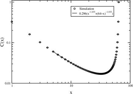
Figure 9: The Greens function $C(x)$ for a system of size $L^{3},L=64$ at $K=K_{c}=0.33305$, $\mu=0$, as a function of $x$. The solid line indicates a power-law fit of the form $0.296(x^{-1.035}+(64-x)^{-1.035}).$

In Figure 9 we show results for the Greens function as a function of $x$ for a system of size $L^{3},L=64$. For this simulation the directed algorithm was used with a total number of worms equal to $1.5\times 10^{8}$. It is easy to obtain extremely small error bars on the Greens functions even for very large system sizes. For the results shown in Fig 9 $\mu=0$ and by symmetry $C(\tau)$ is identical to $C(x)$. From scaling relations Fisher89c $C(r)$ is expected to decay as $r^{-(d-2+z+\eta)}$ where $z$ is the dynamical critical exponent. With $\mu=0$, $z=1$ we find $C(r)\sim r^{-(1+\eta)}$. Fitting to this form we find $\eta=0.035(5)$. The obtained critical exponents are in excellent agreement with previous work Sorensen and more recent high-precision estimates for the critical exponents of the 3d $XY$ model Dukovski .

It would be of much interest to calculate $C({\bf r},\tau)$ for $\mu\neq 0$ using this method. Such calculations are currently in progress muquarter .

VI Summary and discussion

We have proposed a directed worm algorithm for the quantum rotor model. This algorithm is an improvement of the ”undirected” algorithm presented in Alet03 . It has been shown that by adjusting the degrees of freedom left in the detailed balance condition, one can construct a more efficient algorithm by minimizing the back-tracking (bounce) probability for the worm to erase itself. The minimal probabilities can be found by solving a linear programming problem subject to a few well-defined constraints. A proof of detailed balance for the directed case has also been presented. The directed and un-directed algorithms are identical except for the fact that appropriately defined local probabilities $p_{\sigma}$ for moving the worm through the lattice are chosen in an optimal manner for the directed algorithm. Hence, only a very limited amount of additional programming has to be done to implement the directed algorithm.

These central ideas for this directed algorithm can be straightforwardly applied to directed QMC loop algorithms Sylju and one can avoid an analytical calculation for each new model where one wants to implement a directed algorithm. More generally speaking, we believe that the framework presented here could be useful for constructing new algorithms for other models, for example classical spin models Hitchcock .

We have shown the superiority of the directed algorithm as compared to the undirected one and to the approach (”classical worms”) proposed in Prokofev.Classical by calculating autocorrelation times of different observables near a critical point. Whereas the computational gain is not as drastic as when passing from a local update algorithm to a worm algorithm Alet03 ; AletPhD , we showed that one gains a factor ranging from $1.5$ to $10$ (depending on the quantity and on the comparison) for the simulations considered here. We did not try to estimate autocorrelation exponent $z$ for the algorithms, because in all cases, it is small (as can be seen in figure 6) and it would be hard to determine with high precision. Looking at the data, it is likely that values of $z$ for all algorithms are the same or quite close. A logarithmic dependence of $\tau$ on $L$, indicating $z=0$, cannot also be excluded.

In this paper, we have also derived an efficient way of measuring correlation functions during the worm constructions. This feature is similar to other worm algorithms Sandvik ; Prokofev , but here we show, including analytical arguments, that it also works for directed worms. The situation for directed QMC loop algorithms Sylju is less certain, even if some results were recently presented in Ref.roscilde .

The directed worm algorithm could be specially useful to study the transition for a non-commensurate value of the chemical potential in the pure quantum rotor model or for the disordered case, where very strong finite size effects have been identified AletPhD ; muquarter ; Prokofev.QR .

- (1) R. H. Swendsen and J. S. Wang, Phys. Rev. Lett. 58, 86 (1987).
- (2) U. Wolff, Phys. Rev. Lett. 62, 361 (1989).
- (3) H. G. Evertz, G. Lana and M. Marcu, Phys. Rev. Lett. 70, 875 (1993). H. G. Evertz, Adv. Phys. 52, 1 (2003).
- (4) A. W. Sandvik, Phys. Rev. B 59, R14157 (1999); A. Dorneich and M. Troyer, Phys. Rev. E 64, 066701 (2001).
- (5) N. V. Prokof’ev, B. V. Svistunov and I. S. Tupitsyn, Phys. Lett. A 238, 253 (1998).
- (6) F. Alet and E. S. Sørensen, Phys. Rev. E 67, 015701(R) (2003).
- (7) T. Banks, R. Myerson, J. Kogut, Nucl. Phys. B129, 493, (1977); P. R. Thomas, M. Stone, Nucl. Phys. B114, 513 (1978); M. E. Peskin, Ann. Phys. 113, 122 (1978); R. Savit, Rev. Mod. Phys. 52, 453 (1980).
- (8) N. Prokof’ev and B. Svistunov, Phys. Rev. Lett. 87, 160601 (2001).
- (9) O. F. Syljuåsen and A. W. Sandvik, Phys. Rev. E 66, 046701 (2002); K. Harada and N. Kawashima, ibid 66 056705 (2002); O. F. Syljuåsen, Phys. Rev. E 67, 046701 (2003); J. Smakov, K. Harada and N. Kawashima, e-print cond-mat/0301416; F. Alet, S. Wessel and M. Troyer, (unpublished).
- (10) S. Sachdev Quantum Phase Transitions, Cambridge University Press, Cambridge 1999.
- (11) E. S. Sørensen et al., Phys. Rev. Lett. 69, 828 (1992); M. Wallin et al., Phys. Rev. B 49, 12115 (1994).
- (12) M.-C. Cha et al., Phys. Rev. B 44, 6883 (1991).
- (13) A. vanOtterlo and K.-H. Wagenblast, Phys. Rev. Lett. 72, 3598 (1994); A. vanOtterlo et al., Phys. Rev. B 52, 16176 (1995).
- (14) J. Kisker and H. Rieger, Phys. Rev. B 55, R11981 (1997), Physica A 246, 348 (1997);
- (15) S. Y. Park et al., Phys. Rev. B 59, 8420 (1999); J.-W. Lee, M.-C. Cha and D. Kim, Phys. Rev. Lett. 87, 247006 (2001).
- (16) A. B. Bortz, M. H. Kalos and J. L. Lebowitz, J. Comp. Physics, 17, 10 (1975).
- (17) F. Alet, PhD thesis, Université Paul Sabatier, Toulouse (2002).
- (18) Numerical Recipes in C++, W. Press et al., Cambridge University Press (2002).
- (19) N. V. Prokof’ev and B. V. Svistunov, e-print cond-mat/0301205.
- (20) See I. Dukovski, J. Machta and L. V. Chayes, Phys. Rev. E, 65, 026702 (2002) and references there in.
- (21) M. P. A. Fisher, P. B. Weichman, G. Grinstein, and D. S. Fisher, Phys. Rev. B 40, 546 (1989).
- (22) F. Alet and E. S. Sørensen, (unpublished).
- (23) P. Hitchcock, F. Alet and E. Sørensen, (unpublished).
- (24) A. Cuccoli et al., Phys. Rev. B 67, 104414 (2003).