The gap equations for spin singlet and triplet ferromagnetic superconductors

Abstract

We derive gap equations for superconductivity in coexistence with ferromagnetism. We treat singlet states and triplet states with either equal spin pairing (ESP) or opposite spin pairing (OSP) states, and study the behaviour of these states as a function of exchange splitting. For the s-wave singlet state we find that our gap equations correctly reproduce the Clogston–Chandrasekhar limiting behaviour and the phase diagram of the Baltensperger–Sarma equation (excluding the FFLO region). The singlet superconducting order parameter is shown to be independent of exchange splitting at zero temperature, as is assumed in the derivation of the Clogston–Chandrasekhar limit. P-wave triplet states of the OSP type, behave similarly to the singlet state as a function of exchange splitting. On the other hand, ESP triplet states show a very different behaviour. In particular there is no Clogston–Chandrasekhar limiting and the superconducting critical temperature, $T_{C}$, is actually increased by exchange splitting.

1 Introduction

The recent discovery of the coexistence of ferromagnetism and superconductivity in UGe₂ [1] URhGe [2] and ZrZn₂ [3] has led to renewed interest in the relationship between ferromagnetism and superconductivity. By contrast, the relationship between antiferromagnetism and superconductivity has been more thoroughly studied [4], since it is relevant to many compounds, such as the cuprates [5], borocarbides [6], heavy Fermion superconductors [7] and the layered organic superconductors [8].

Particular interest has been focused on superconductivity on the border of a magnetic phase and in particular in the vicinity of a quantum critical point (QCP). This is observed experimentally in cuprates, several heavy Fermion systems, layered organics and UGe₂. It is also thought that URhGe₂ may be essentially similar to UGe₂ but under the influence of ‘chemical pressure’ [2]. Similarly, the ferromagnetism in ZrZn₂ also shows a QCP at high pressures. But in this case, unlike UGe₂, the highest superconducting transition temperatures are observed at ambient pressure, that is at the furthest point from the ferromagnetic-paramagnetic QCP.

Theoretically it is thought that at or near to the QCP quantum spin fluctuations, can lead to spin-fluctuation induced pairing. For the case of ferromagnetic QCP this was first studied by Fay and Appel [9] (who also suggested that ZrZn₂ might be a suitable system in which to observe this effect). In this case the ferromagnetic spin fluctuations lead to spin-triplet pairing, by analogue with the case of superfluid ³He. By contrast, in the case of quantum critical antiferromagnetic spin fluctuations spin-singlet d-wave pairing states are favoured [5].

Currently, very little is known about the superconducting pairing state in the ferromagnetic superconductors UGe₂, URhGe and ZrZn₂. If the pairing mechanism is indeed caused by ferromagnetic spin fluctuations, then we might expect spin-triplet pairing states. However, presently there is insufficient evidence in support of this hypothesis to be decisive. Thus it is still legitimate to consider other scenarios. In fact this is what we shall do here. In short, we point out that the decline of the superconducting transition temperature, $T_{c}$, with pressure could be a simple consequence of p-wave pairing of arbitrary origin in an exchange field.

In particular we will consider a simple model of the coexistence between ferromagnetism and superconductivity based on a parameterised electron-electron attractive interaction of unspecified origin. We will derive Bogoliubov–de Gennes (BdG) and gap equations for this model using the Hartree–Fock–Gorkov approximation. We will consider separately the cases of: spin singlet (s-wave) pairing, Opposite Spin Pairing (OSP) and Equal Spin Pairing (ESP) spin triplet (p-wave) states. Solving the gap equations for these pairing states, we will then illustrate some important properties of superconductivity in the presence of ferromagnetism.

2 A simple model for a ferromagnetic superconductor

We consider superconductivity arising in a Hubbard model with an effective attractive pairwise interaction $U_{ij\sigma\sigma^{\prime}}$, acting between electrons at crystal sites $i$, $j$ with spins $\sigma$ and $\sigma^{\prime}$. In principle this effective interaction could arise from either conventional pairing mechanisms, such as electron-phonon coupling, or exchange of spin-fluctuations. Here we shall assume that the effective interaction is both short-ranged in space, namely $U_{ij\sigma\sigma^{\prime}}\neq 0$ only for $i=j$ or nearest neighbours, and non-retarded.

In the ferromagnetic state we must also include the effective exchange field caused by the ferromagnetism. This enters in the model Hamiltonian as to the Zeeman splitting $\bi{V}_{xc}$. Thus the complete Hamiltonian for this model is

$$\hat{\cal{H}}=-\sum_{ij\sigma}t_{ij}\hat{c}_{i\sigma}^{\dagger}\hat{c}_{j\sigma}+\frac{1}{2}\sum_{ij\sigma\sigma^{\prime}}U_{ij\sigma\sigma^{\prime}}\hat{n}_{i\sigma}\hat{n}_{j\sigma^{\prime}}+\sum_{i\sigma\sigma^{\prime}}\hat{c}_{i\sigma}^{\dagger}(\bi{\sigma}_{\sigma\sigma^{\prime}}\cdot\bi{V}_{xc})\hat{c}_{i\sigma}$$ (1)

where the $\hat{c}_{i\sigma}^{({\dagger})}$ are the usual annihilation (creation) operators, $\hat{n}_{i\sigma}$ is the number operator and the $\bi{\sigma}_{\sigma\sigma^{\prime}}$ are the components of the vector of Pauli matrices

$$\underline{\underline{\bi{\sigma}}}=(\underline{\underline{\sigma}}_{1},\underline{\underline{\sigma}}_{2},\underline{\underline{\sigma}}_{3}).$$ (2)

In this context we should note that the ferromagnetism of ZrZn₂ is accurately described by the LSDA as a weak itinerant ferromagnet. Experimentally the exchange splitting is clearly resolved in de Haas-van Alphen experiments [10] and band structure calculations (also presented in reference [10]) are in excellent agreement with these experiments. Moreover, the calculated moment (0.18$\mu_{B}$) is close to the observed moment (0.17$\mu_{B}$). Both the Curie temperature, $T_{FM}$, and low temperature magnetisation are linear functions of pressure [11]. Hence the low temperature magnetisation is a linear function of $T_{FM}$, in line with the predictions of the Stoner model. The most unusual magnetic property of ZrZn₂ is that, although a field of 0.05 T is enough to form a single magnetic domain, the ordered moment is unsaturated up to 35 T [3, 12]. This is far more naturally understood in an itinerant model such as LSDA or the Stoner model than, say, the Heisenberg model. On the other hand, we hasten to add that it is not clear whether this picture is useful for the ferromagnetic superconductor UGe₂, since there the moments are much more strongly localised.

Making the usual Hartree-Fock–Gorkov approximation, such that $\Delta_{ij\sigma\sigma^{\prime}}=-U_{ij\sigma\sigma^{\prime}}\langle\hat{c}_{i\sigma}\hat{c}_{j\sigma^{\prime}}\rangle$, and using the spin-generalised Bogoliubov–Valatin transformation,

$$\hat{c}_{i\sigma}=\sum_{\bi{k}\sigma^{\prime}}u_{\bi{k}\sigma\sigma^{\prime}}(\bi{R}_{i})\hat{\gamma}_{\bi{k}\sigma^{\prime}}+v_{\bi{k}\sigma\sigma^{\prime}}^{*}(\bi{R}_{i})\hat{\gamma}_{\bi{k}\sigma^{\prime}}^{\dagger}$$ (3)

subject to the completeness relation

$$\sum_{\bi{k}\sigma}\left(u_{\bi{k}\alpha\sigma}^{*}(\bi{R}_{i})u_{\bi{k}\beta\sigma}(\bi{R}_{j})+v_{\bi{k}\alpha\sigma}(\bi{R}_{i})v_{\bi{k}\beta\sigma}^{*}(\bi{R}_{j})\right)=\delta_{ij}\delta_{\alpha\beta},$$ (4)

we find that the Bogoliubov de Gennes (BdG) equations for this Hamiltonian are

$$\left(\begin{array}[]{cccc}\varepsilon_{\bi k}+V_{xc3}&V_{xc1}-\rmi V_{xc2}&\Delta_{\uparrow\uparrow}({\bi{k}})&\Delta_{\uparrow\downarrow}(\bi{k})\\ V_{xc1}+\rmi V_{xc2}&\varepsilon_{\bi{k}}-V_{xc3}&\Delta_{\downarrow\uparrow}({\bi{k}})&\Delta_{\downarrow\downarrow}({\bi{k}})\\ -\Delta_{\uparrow\uparrow}^{*}(-\bi{k})&-\Delta_{\uparrow\downarrow}^{*}(-\bi{k})&-\varepsilon_{-\bi{k}}-V_{xc3}&-V_{xc1}-\rmi V_{xc2}\\ -\Delta_{\downarrow\uparrow}^{*}(-\bi{k})&-\Delta_{\downarrow\downarrow}^{*}(-\bi{k})&-V_{xc1}+\rmi V_{xc2}&-\varepsilon_{-\bi{k}}+V_{xc3}\end{array}\right)\left(\begin{array}[]{c}u_{\uparrow\sigma}({\bi{k}})\\ u_{\downarrow\sigma}({\bi{k}})\\ v_{\uparrow\sigma}({\bi{k}})\\ v_{\downarrow\sigma}({\bi{k}})\end{array}\right)$$ (13)

$$=E_{\sigma}({\bi{k}})\left(\begin{array}[]{c}u_{\uparrow\sigma}({\bi{k}})\\ u_{\downarrow\sigma}({\bi{k}})\\ v_{\uparrow\sigma}({\bi{k}})\\ v_{\downarrow\sigma}({\bi{k}})\end{array}\right)$$ (18)

where $\varepsilon_{\bi{k}}$ is the normal (that is non superconducting and non ferromagnetic) state energy and $\bi{V}_{xc}=(V_{xc1},V_{xc2},V_{xc3})$.

The superconducting order parameter, $\Delta_{\sigma\sigma^{\prime}}(\bi{k})$, is calculated self-consistently from

$$\Delta_{\sigma\sigma^{\prime}}({\bf k})=-\frac{1}{2}\sum_{\bi{q}\sigma^{\prime\prime}}U_{\sigma\sigma^{\prime}}(\bi{k}-\bi{q})\Big{(}u_{\sigma\sigma^{\prime\prime}}(-\bi{q})v^{\ast}_{\sigma^{\prime}\sigma^{\prime\prime}}(-\bi{q})-v^{\ast}_{\sigma\sigma^{\prime\prime}}(\bi{q})u_{\sigma^{\prime}\sigma^{\prime\prime}}(\bi{q})\Big{)}(1-2f_{E_{\bi{q}\sigma^{\prime\prime}}}).$$ (19)

We now introduce the Balain-Werthamer (BW) transformation [13, 14],

$$\underline{\underline{\Delta}}({\bi{k}})\equiv\left(\begin{array}[]{cc}\Delta_{\uparrow\uparrow}(\bi{k})&\Delta_{\uparrow\downarrow}({\bi{k}})\\ \Delta_{\downarrow\uparrow}({\bi{k}})&\Delta_{\downarrow\downarrow}({\bi{k}})\end{array}\right)=\left(d_{0}(\bi{k})+\underline{\underline{\sigma}}\cdot\bi{d}(\bi{k})\right)\rmi\underline{\underline{\sigma_{2}}}.$$ (20)

which separates the superconducting order parameter into a singlet (scalar) part, $d_{0}(\bi{k})$ and a triplet (vector) part, $\bi{d}(\bi{k})=(d_{1}(\bi{k}),d_{2}(\bi{k}),d_{3}(\bi{k}))$. In terms of these parameters the BdG equations can be rewritten as

$$\left(\begin{array}[]{cccc}\varepsilon_{\bi k}+V_{xc3}&V_{xc1}-\rmi V_{xc2}&-d_{1}(\bi{k})+\rmi d_{2}({\bi{k}})&d_{0}({\bi{k}})+d_{3}({\bi{k}})\\ V_{xc1}+\rmi V_{xc2}&\varepsilon_{\bi{k}}-V_{xc3}&-d_{0}({\bi{k}})+d_{3}({\bi{k}})&d_{1}({\bi{k}})+\rmi d_{2}({\bi{k}})\\ -d^{\ast}_{1}({\bi{k}})-\rmi d^{\ast}_{2}({\bi{k}})&-d^{\ast}_{0}({\bi{k}})+d^{\ast}_{3}({\bi{k}})&-\varepsilon_{-\bi{k}}-V_{xc3}&-V_{xc1}-\rmi V_{xc2}\\ d^{\ast}_{0}({\bi{k}})+d^{\ast}_{3}({\bi{k}})&d^{\ast}_{1}({\bi{k}})-\rmi d^{\ast}_{2}({\bi{k}})&-V_{xc1}+\rmi V_{xc2}&-\varepsilon_{-\bi{k}}+V_{xc3}\end{array}\right)$$ (25)

$$\left(\begin{array}[]{c}u_{\uparrow\sigma}({\bi{k}})\\ u_{\downarrow\sigma}({\bi{k}})\\ v_{\uparrow\sigma}({\bi{k}})\\ v_{\downarrow\sigma}({\bi{k}})\end{array}\right)=E_{\sigma}({\bi{k}})\left(\begin{array}[]{c}u_{\uparrow\sigma}({\bi{k}})\\ u_{\downarrow\sigma}({\bi{k}})\\ v_{\uparrow\sigma}({\bi{k}})\\ v_{\downarrow\sigma}({\bi{k}})\end{array}\right)$$ (34)

Using this formalism, it is also possible to calculate the free energy in the general case. This is given by

$$F=\sum_{\bi{k}\alpha\sigma}\varepsilon{k}\Big{(}u_{\alpha\sigma}^{*}(-\bi{k})u_{\alpha\sigma}(-\bi{k})f_{\bi{k}\sigma}+v_{\alpha\sigma}(\bi{k})v_{\alpha\sigma}^{*}(\bi{k})\big{(}1-f_{\bi{k}\sigma}\big{)}\Big{)}$$

$$-\frac{1}{2}\sum_{\bi{k}\bi{k}^{\prime}\alpha\beta\sigma\sigma^{\prime}}\Bigg{(}U(\bi{k}-\bi{k}^{\prime})$$

$$\times\Big{[}u_{\alpha\sigma}^{*}(-\bi{k})v_{\beta\sigma}(\bi{k})f_{\bi{k}\sigma}+v_{\alpha\sigma}(-\bi{k})u_{\beta\sigma}^{*}(\bi{k})\big{(}1-f_{\bi{k}\sigma}\big{)}\Big{]}$$

$$\times\Big{[}u_{\alpha\sigma^{\prime}}(-\bi{k}^{\prime})v_{\beta\sigma^{\prime}}^{*}(\bi{k}^{\prime})f_{\bi{k}^{\prime}\sigma^{\prime}}+v_{\alpha\sigma^{\prime}}^{*}(-\bi{k}^{\prime})u_{\beta\sigma^{\prime}}(\bi{k}^{\prime})\big{(}1-f_{\bi{k}^{\prime}\sigma^{\prime}}\big{)}\Big{]}\Bigg{)}$$

$$+\sum_{\bi{k}\alpha\beta\sigma}\big{(}\bi{\sigma}_{\alpha\beta}\cdot\bi{H}\big{)}\Big{(}u_{\alpha\sigma}^{*}(\bi{k})u_{\beta\sigma}(\bi{k})f_{\bi{k}\sigma}+v_{\alpha\sigma}(\bi{k})v_{\alpha\sigma}^{*}(\bi{k})\big{(}1-f_{\bi{k}\sigma}\big{)}\Big{)}$$

$$-k_{B}T\sum_{\bi{k}\sigma}\Big{[}f_{\bi{k}\sigma}\ln{f_{\bi{k}\sigma}}+\big{(}1-f_{\bi{k}\sigma}\big{)}\ln{\big{(}1-f_{\bi{k}\sigma}\big{)}}\Big{]}$$ (35)

At this stage one must resort either to solving these equations numerically [15, 16], or to studying special cases. In this paper we shall take the later approach. First, we begin by considering the case singlet pairing only (i.e. $d_{1}(\bi{k})=d_{2}(\bi{k})=d_{3}(\bi{k})=0$). In section 4 we will consider the case of only triplet pairing (i.e. when $d_{0}(\bi{k})=0$).

3 The coexistence of singlet superconductivity and ferromagnetism

In the case of a s-wave spin singlet superconductor, it was shown by Fulde, Ferrel, Larkin and Ovchinnikov (FFLO) [17, 18] that the superconducting ground state becomes non-uniform for small external exchange fields. This solution is well known, and we shall not study it here. On the other hand there are also solutions which are spatially uniform. Whichever of these solutions is the ground state can only be determined by calculating the free energy for both and finding which is the lower solution. In strong fields the FFLO state will be the minimum, but in weaker fields the FFLO state will be unstable to the uniform solution. In the rest of this section we study the gap equations for the spatially uniform case.

It is straightforward to show that $d_{0}(\bi{k})$ transforms as a scalar under spin rotation. Thus, if there is no superconductivity in the triplet channel, we can, without loss of generality, rewrite the BdG equations as

$$\left(\begin{array}[]{cccc}\varepsilon_{\bi k}+V_{xc}&0&0&d_{0}({\bi{k}})\\ 0&\varepsilon_{\bi{k}}-V_{xc}&-d_{0}({\bi{k}})&0\\ 0&-d^{\ast}_{0}({\bi{k}})&-\varepsilon_{-\bi{k}}-V_{xc}&0\\ d^{\ast}_{0}({\bi{k}})&0&0&-\varepsilon_{-\bi{k}}+V_{xc}\end{array}\right)\left(\begin{array}[]{c}u_{\uparrow\sigma}({\bi{k}})\\ u_{\downarrow\sigma}({\bi{k}})\\ v_{\uparrow\sigma}({\bi{k}})\\ v_{\downarrow\sigma}({\bi{k}})\end{array}\right)$$ (44)

$$=E_{\sigma}({\bi{k}})\left(\begin{array}[]{c}u_{\uparrow\sigma}({\bi{k}})\\ u_{\downarrow\sigma}({\bi{k}})\\ v_{\uparrow\sigma}({\bi{k}})\\ v_{\downarrow\sigma}({\bi{k}})\end{array}\right).$$ (49)

by rotating our spin reference frame so that $V_{xc}=\sqrt{{V_{xc1}}^{2}+{V_{xc2}}^{2}+{V_{xc3}}^{2}}$.

Equation (49) can be separated into two sets of BdG equations, so we have

$$\left(\begin{array}[]{cc}\varepsilon_{\bi{k}}+V_{xc}&d_{0}({\bi{k}})\\ d^{\ast}_{0}({\bi{k}})&-\varepsilon_{\bi{k}}+V_{xc}\end{array}\right)\left(\begin{array}[]{c}u_{\uparrow\uparrow}({\bi{k}})\\ v_{\downarrow\uparrow}({\bi{k}})\end{array}\right)=E_{\uparrow}({\bi{k}})\left(\begin{array}[]{c}u_{\uparrow\uparrow}({\bi{k}})\\ v_{\downarrow\uparrow}({\bi{k}})\end{array}\right)$$ (50)

and

$$\left(\begin{array}[]{cc}\varepsilon_{\bi{k}}-V_{xc}&-d_{0}({\bi{k}})\\ -d^{\ast}_{0}({\bi{k}})&-\varepsilon_{\bi{k}}-V_{xc}\end{array}\right)\left(\begin{array}[]{c}u_{\downarrow\downarrow}({\bi{k}})\\ v_{\uparrow\downarrow}({\bi{k}})\end{array}\right)=E_{\downarrow}({\bi{k}})\left(\begin{array}[]{c}u_{\downarrow\downarrow}({\bi{k}})\\ v_{\uparrow\downarrow}({\bi{k}})\end{array}\right).$$ (51)

Figure 1: The four branches of the singlet spectrum in a magnetic field. Inset, the zero field limit where the two spin branches become degenerate. The branches are (a) the spectra for $\sigma=\uparrow$, (b) the spectra for $\sigma=\downarrow$, (c) the normal state spectra in zero field and (d) the singlet spectrum for $V_{xc}=0$.

It is now a simple matter to regain the standard result [19] for the spectrum of a singlet superconductor in a spin only magnetic field:

$$E_{\sigma}(\bi{k})=\sqrt{\varepsilon_{\bi{k}}^{2}+|d_{0}(\bi{k})|^{2}}+\sigma|\bi{V}_{xc}|,$$ (52)

with $\sigma=\uparrow\,\equiv 1$ and $\sigma=\downarrow\,\equiv-1$. The four corresponding energy levels are sketched in Fig, 1. Equation (52) clearly reduces to the standard BCS expression for the spectrum of a singlet superconductor in the absence of exchange splitting as $V_{xc}\rightarrow 0$. Also, when $V_{xc}=0$ equations (50) and (51) reduce to the usual BdG equations [20] and we see that we are justified in associating $d_{0}(\bi{k})$ with the usual singlet superconducting order parameter $\Delta(\bi{k})$.

It is clear from (49) that

$$u_{\sigma-\sigma}(\bi{k})=v_{\sigma\sigma}(\bi{k})=0,$$ (53)

and it can also be shown that

$$u_{\sigma\sigma}(\bi{k})=\frac{d_{0}(\bi{k})}{\sqrt{(E_{0}(\bi{k})-\varepsilon_{\bi{k}})^{2}+|d_{0}(\bi{k})|^{2}}}$$ (54)

and

$$v_{\sigma-\sigma}(\bi{k})=\frac{E_{0}(\bi{k})-\varepsilon_{\bi{k}}}{\sqrt{(E_{0}(\bi{k})-\varepsilon_{\bi{k}})^{2}+|d_{0}(\bi{k})|^{2}}}$$ (55)

where

$$E_{0}(\bi{k})=\sqrt{\varepsilon_{\bi{k}}+|d_{0}(\bi{k})|^{2}}.$$ (56)

$E_{0}(\bi{k})$ is, of course, of the same mathematical form as the spectrum of a singlet superconductor in the absence of exchange splitting. However, it is not correct to say that $E_{0}(\bi{k})$ is the spectrum of a singlet superconductor in the absence of exchange splitting as the value of $d_{0}(\bi{k})$ (although, importantly, not the value of $\varepsilon(\bi{k})$) depends on $V_{xc}$ in general.

Substituting our expressions for the eigenvectors of the BdG into the self-consistency condition (19) we find that the gap equation is

$$d_{0}(\bi{k})=-\frac{1}{4}\sum_{\bi{k}\sigma}U_{\sigma-\sigma}(\bi{k})\frac{d_{0}(\bi{k})}{E_{0}(\bi{k})}\tanh\left(\frac{E_{0}(\bi{k})+\sigma V_{xc}}{2k_{B}T}\right).$$ (57)

In the absence of exchange splitting the gap equation regains its familiar BCS form [21]. However, we note that surprisingly the exchange splitting dependence of the gap only enters via the Fermi ($\tanh$) term. This means that when $T=0$ the gap equation becomes

$$d_{0}(\bi{k})=-\frac{1}{4}\sum_{\bi{k}\sigma}U_{\sigma-\sigma}(\bi{k})\frac{d_{0}(\bi{k})}{E_{0}(\bi{k})}.$$ (58)

which is independent of $\bi{V}_{xc}$.

We must now ask what this result means physically. The most obvious conclusion is that, at zero temperature, the gap in independent of exchange splitting. This is true, but with one condition, which we will discuss below.

The gap equation is a non-linear integral equation. And, as such, has, in general, more than one solution. (For example the trivial solution $d_{0}(\bi{k})=0$ is always a solution.) All that we have actually shown is that for any given solution $d_{0}(\bi{k})$ is independent $\bi{V}_{xc}$ at $T=0$. To find the ground state we must consider all possible solutions and calculate the free energy of each solution. In the absence of exchange splitting the gap equation can be derived by minimising the free energy with respect to the superconducting order parameter [22]. This leads to the conclusion that the trivial solution is only the ground state when no other solution exists. However, no such proof exists for a superconductor in a finite exchange splitting. This means that it is perfectly possible there to be a phase transition from the superconducting to normal states as the exchange splitting is increased at zero temperature. Any such phase transition will be ‘perfectly’ first order in the sense that the order parameter will jump from zero (above the critical exchange splitting, $V_{xc}^{C}$) to some finite value (below $V_{xc}^{C}$) and remain at that value for all $V_{xc}\leq V_{xc}^{C}$. The order parameter as a function of exchange splitting will therefore resemble a Heaviside step function. Of course, as in general other superconducting phases can exist (such as the FFLO state) phase transitions can also occur between different superconducting phases in a similar manner [23].

Such a phase transition was first studied independently by Clogston [24] and Chandrasekhar [25] who both, in fact, assumed the independence of $d_{0}(\bi{k})$ on $V_{xc}$ that we have derived above. Using this assumption they were able to show from simple thermodynamics that if the exchange splitting is greater than $V_{xc}^{P}\equiv|\Delta(0)|/\sqrt{2}$ where $|\Delta(0)|$ is the superconducting gap at zero temperature (and zero exchange splitting) then the normal state has a lower energy than the s-wave superconducting state. This is known both of as Clogston–Chandrasekhar limiting and as Pauli-paramagnetic limiting. Clogston–Chandrasekhar limiting clearly applies to all singlet states, but does not necessarily apply to triplet states. In most superconducting materials $\mu_{B}H_{C2}<V_{xc}^{P}$. Therefore, if a superconductor has a large upper critical field in comparison to the Clogston–Chandrasekhar limit this is good evidence for triplet superconductivity. The FFLO state can also display $\mu_{B}H_{C2}>V_{xc}^{P}$. Clogston–Chandrasekhar limiting has been observed in the layered organic compound $\kappa-$(BEDT-TTF)₂Cu(SCN)₂ [26] when a magnetic field is applied parallel to the layers (which prevents the formation of orbital currents due to the highly two dimensional nature of the material).

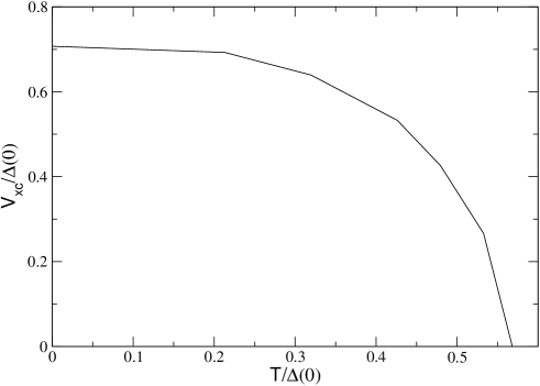
Figure 2: The phase diagram of an s-wave superconductor in an exchange field calculated by solving the spin generalised BdG equations self consistently. Note that as the phase transition is first order in the presence of exchange splitting the free energy must be calculated for both the normal and superconducting states to correctly construct this phase diagram.

To illustrate this point, we have solved the gap equation (57) numerically for a cubic lattice. We assumed $U_{ij\sigma\sigma}=U\delta_{ij}$ (i.e. an on-site interaction) corresponding to the case of local s-wave pairing. The comparison between the calculated superconducting and normal state free energies, leads to the phase diagram given in figure 2. This calculated phase diagram is in excellent agreement with that calculated from the Baltensperger–Sarma equation [27, 28]. However, while the Baltensperger–Sarma equation only allows for the calculation of the superconducting-metal phase transition, our numerical gap equation solution allows for the evaluation of the order parameter at any point in $T-V_{xc}$ space and hence for the evaluation of thermodynamic variables such as the heat capacity,

$$C_{V}=\sum_{\bi{k}\sigma}\frac{1}{k_{B}T^{2}}f_{\bi{k}\sigma}\big{(}1-f_{\bi{k}\sigma}\big{)}\left(E_{\bi{k}\sigma}^{2}-\frac{1}{E_{\bi{k}\sigma}-\sigma V_{xc}}\frac{\partial|d_{0}(\bi{k})|^{2}}{\partial T}\right).$$ (59)

and the magnetisation [19],

$$M=-\frac{V}{(2\pi)^{3}}\sum_{\sigma}\sigma\int\rmd^{3}\bi{k}\frac{1}{1+e^{(E_{\bi{k}\sigma}-\mu)/k_{B}T}}.$$ (60)

where $V$ is the volume of the first Brillouin zone.

A numerical study of these equations [16] shows that, in an exchange field, the thermodynamic functions ‘see’ an effective gap, $\Delta_{eff}$, i.e.

$$\{C_{V},M,\chi\}\sim e^{-\frac{\Delta_{eff}}{k_{B}T}}$$ (61)

where

$$\Delta_{eff}=|\Delta(0)|-|\bi{V}_{xc}|.$$ (62)

4 The coexistence of triplet superconductivity and ferromagnetism

We will now consider the properties of a triplet superconductor in a magnetic field. Using a similar approach to the singlet case above we are able to derive many of the same physical quantities. This highlights both similarities and differences between the singlet and triplet cases, which may perhaps help in identifying the pairing state symmetry in specific ferromagnetic superconductors.

Before we begin we will generalise a useful theorem due to de Gennes [20]. We begin by writing the BdG equations (18) in a pseudo-spinor notation:

$$\left(\begin{array}[]{cc}\underline{\underline{\xi}}({\bi{k}})&\underline{\underline{\Delta}}_{\bi{k}}\\ -\underline{\underline{\Delta}}^{*}_{-\bi{k}}&-\underline{\underline{\xi}}^{*}({\bi{k}})\end{array}\right)\left(\begin{array}[]{c}\underline{u}_{\sigma}({\bi{k}})\\ \underline{v}_{\sigma}({\bi{k}})\end{array}\right)=E_{\sigma}({\bi{k}})\left(\begin{array}[]{c}\underline{u}_{\sigma}({\bi{k}})\\ \underline{v}_{\sigma}({\bi{k}})\end{array}\right).$$ (63)

Where

$$\underline{\underline{\xi}}({\bi{k}}) = \left(\begin{array}[]{cc}\varepsilon_{\bi k}+V_{xc3}&V_{xc1}-\rmi V_{xc2}\\ V_{xc1}+\rmi V_{xc2}&\varepsilon_{\bi{k}}-V_{xc3}\end{array}\right),$$ (66)

$$\underline{\underline{\Delta}}_{\bi{k}} = \left(\begin{array}[]{cc}\Delta_{\uparrow\uparrow}({\bi{k}})&\Delta_{\uparrow\downarrow}(\bi{k})\\ \Delta_{\downarrow\uparrow}({\bi{k}})&\Delta_{\downarrow\downarrow}({\bi{k}})\end{array}\right),$$ (69)

$$\underline{u}_{\sigma}({\bi{k}}) = \left(\begin{array}[]{cc}u_{\uparrow\sigma}({\bi{k}})\\ u_{\downarrow\sigma}({\bi{k}})\end{array}\right),$$ (72)

and

$$\underline{v}_{\sigma}({\bi{k}}) = \left(\begin{array}[]{cc}v_{\uparrow\sigma}({\bi{k}})\\ v_{\downarrow\sigma}({\bi{k}})\end{array}\right).$$ (75)

Multiplying by $-1$, taking the complex conjugate, parity inverting and exchanging the rows of (63) leads to

$$\left(\begin{array}[]{cc}\underline{\underline{\xi}}({\bi{k}})&\underline{\underline{\Delta}}({\bi{k}})\\ -\underline{\underline{\Delta}}^{*}({\bi{k}})&-\underline{\underline{\xi}}^{*}({\bi{-k}})\end{array}\right)\left(\begin{array}[]{c}\underline{u}^{*}_{\sigma}({\bi{-k}})\\ \underline{v}^{*}_{\sigma}({\bi{-k}})\end{array}\right)=-E_{\sigma}({\bi{k}})\left(\begin{array}[]{c}\underline{u}^{*}_{\sigma}({\bi{-k}})\\ \underline{v}^{*}_{\sigma}({\bi{-k}})\end{array}\right),$$ (76)

as both $E_{\sigma}({\bi{k}})$ and $\underline{\underline{\xi}}({\bi{k}})$ are even under parity inversion.

We have therefore shown that if $\left(\begin{array}[]{c}\underline{u}_{\sigma}({\bi{k}})\\ \underline{v}_{\sigma}({\bi{k}})\end{array}\right)$ is an eigenvector of the spin-generalised BdG equations in a magnetic field, with the corresponding eigenvalue $E_{\sigma}({\bi{k}})$ then, $\left(\begin{array}[]{c}\underline{u}^{*}_{\sigma}({\bi{-k}})\\ \underline{v}^{*}_{\sigma}({\bi{-k}})\end{array}\right)$ is also an eigenvector and that the corresponding eigenvalue is $-E_{\sigma}({\bi{k}})$. As $\sigma$ can take two values ($\uparrow$ or $\downarrow$) we have identified all of the eigenstates.

This analysis holds for both triplet and singlet states. (For a singlet state with $|\bi{V}_{xc}|=0$ it clearly reduces to the theorem of de Gennes.) The spectrum for a singlet superconductor in an exchange field (shown in figure 1) is clearly in agreement with this theorem.

When studying triplet states, and particularly when studying the effect of exchange splitting on the triplet state, it is useful to introduce the notion of unitary and non-unitary states. For a triplet state

$$\underline{\underline{\Delta}}{k}\,\underline{\underline{\Delta}}{k}^{\dagger}=\underline{\underline{I}}\,|\bi{d}(\bi{k})|^{2}+\rmi\bi{\underline{\underline{\sigma}}}\cdot(\bi{d}(\bi{k})\times\bi{d}(\bi{k})^{*})$$ (77)

and, in the absence of exchange splitting,

$$E_{\sigma}(\bi{k})=\sqrt{\varepsilon{k}^{2}+|\bi{d}(\bi{k})|^{2}+\sigma|\bi{d}(\bi{k})\times\bi{d}(\bi{k})^{*}|}.$$ (78)

It is therefore useful to introduce the vector $\bi{q}(\bi{k})$ which is defined by

$$\bi{q}(\bi{k})=\rmi\bi{d}(\bi{k})\times\bi{d}(\bi{k})^{*}.$$ (79)

It is clear that $\bi{q}(\bi{k})$ is a real vector. A unitary state is defined as any state in which $\bi{q}(\bi{k})=0$ for all $\bi{k}$.

By setting the singlet order parameter, $d_{0}(\bi{k})$, to zero we can write down the BdG equations for a triplet superconductor in an exchange field,

$$\left(\begin{array}[]{cccc}\varepsilon_{\bi{k}}+V_{xc3}&V_{xc1}-\rmi V_{xc2}&-d_{1}(\bi{k})+\rmi d_{2}({\bi{k}})&d_{3}({\bi{k}})\\ V_{xc1}+\rmi V_{xc2}&\varepsilon_{\bi{k}}-V_{xc3}&d_{3}({\bi{k}})&d_{1}({\bi{k}})+\rmi d_{2}({\bi{k}})\\ -d^{\ast}_{1}({\bi{k}})-\rmi d^{\ast}_{2}({\bi{k}})&d^{\ast}_{3}({\bi{k}})&-\varepsilon_{\bi{k}}-V_{xc3}&-V_{xc1}-\rmi V_{xc2}\\ d^{\ast}_{3}({\bi{k}})&d^{\ast}_{1}({\bi{k}})-\rmi d^{\ast}_{2}({\bi{k}})&-V_{xc1}+\rmi V_{xc2}&-\varepsilon_{\bi{k}}+V_{xc3}\end{array}\right)$$ (84)

$$\left(\begin{array}[]{c}u_{\uparrow\sigma}({\bi{k}})\\ u_{\downarrow\sigma}({\bi{k}})\\ v_{\uparrow\sigma}({\bi{k}})\\ v_{\downarrow\sigma}({\bi{k}})\end{array}\right)=E_{\sigma}({\bi{k}})\left(\begin{array}[]{c}u_{\uparrow\sigma}({\bi{k}})\\ u_{\downarrow\sigma}({\bi{k}})\\ v_{\uparrow\sigma}({\bi{k}})\\ v_{\downarrow\sigma}({\bi{k}})\end{array}\right).\hskip 15.0pt$$ (93)

The eigenvalues of these BdG equations are given by [16]

$$E_{\sigma}(\bi{k})=\sqrt{\varepsilon_{\bi{k}}^{2}+\mu_{B}^{2}|\bi{V}_{xc}|^{2}+|\bi{d}(\bi{k})|^{2}+\sigma\sqrt{\Lambda(\bi{k})}}$$ (94)

where

$$\Lambda(\bi{k})=|\bi{q}(\bi{k})|^{2}+4\varepsilon_{\bi{k}}^{2}\mu_{B}^{2}|\bi{V}_{xc}|^{2}+4\mu_{B}^{2}|\bi{V}_{xc}\cdot\bi{d}(\bi{k})|^{2}+4\varepsilon_{\bi{k}}\mu_{B}\bi{V}_{xc}\cdot\bi{q}(\bi{k}).$$ (95)

In zero field we clearly have the usual result (78) for the spectrum a triplet superconductor.

Again, we can also derive the expressions for thermodynamic quantities in a general triplet state. For example the heat capacity is given by

$$C_{V}=\sum_{\bi{k}\sigma}\frac{f_{\bi{k}\sigma}(1-f_{\bi{k}\sigma})}{k_{B}T^{2}}\left(E_{\sigma}(\bi{k})^{2}-\frac{T}{2}\frac{d}{dT}|\bi{d}(\bi{k})|^{2}\right)$$ (96)

and the (vector) magnetisation, $\bi{M}$, is given by

$$\bi{M}=\sum_{\bi{k}}\bigg{(}u_{\uparrow\sigma}^{*}(\bi{k})u_{\downarrow\sigma}(\bi{k})f_{\bi{k}\sigma}+v_{\uparrow\sigma}(\bi{k})v_{\downarrow\sigma}^{*}(\bi{k})\big{(}1-f_{\bi{k}\sigma}\big{)}$$

$$+u_{\downarrow\sigma}^{*}(\bi{k})u_{\uparrow\sigma}(\bi{k})f_{\bi{k}\sigma}+v_{\downarrow\sigma}(\bi{k})v_{\uparrow\sigma}^{*}(\bi{k})\big{(}1-f_{\bi{k}\sigma}\big{)},$$

$$-\rmi u_{\uparrow\sigma}^{*}(\bi{k})u_{\downarrow\sigma}(\bi{k})f_{\bi{k}\sigma}-\rmi v_{\uparrow\sigma}(\bi{k})v_{\downarrow\sigma}^{*}(\bi{k})\big{(}1-f_{\bi{k}\sigma}\big{)}$$

$$+\rmi u_{\downarrow\sigma}^{*}(\bi{k})u_{\uparrow\sigma}(\bi{k})f_{\bi{k}\sigma}+\rmi v_{\downarrow\sigma}(\bi{k})v_{\uparrow\sigma}^{*}(\bi{k})\big{(}1-f_{\bi{k}\sigma}\big{)},$$

$$+u_{\uparrow\sigma}^{*}(\bi{k})u_{\uparrow\sigma}(\bi{k})f_{\bi{k}\sigma}+v_{\downarrow\sigma}(\bi{k})v_{\downarrow\sigma}^{*}(\bi{k})\big{(}1-f_{\bi{k}\sigma}\big{)}$$

$$-u_{\downarrow\sigma}^{*}(\bi{k})u_{\uparrow\sigma}(\bi{k})f_{\bi{k}\sigma}-v_{\downarrow\sigma}(\bi{k})v_{\uparrow\sigma}^{*}(\bi{k})\big{(}1-f_{\bi{k}\sigma}\big{)}\bigg{)}.$$ (97)

Following the methods of Sigrist and Ueda [29] it can be shown [16] that in the absence of exchange splitting the gap equations for a triplet superconductor are

$$\Delta_{\alpha\beta}(\bi{k})=\sum_{\bi{k}^{\prime}}U_{\alpha\beta}(\bi{k}-\bi{k}^{\prime})\left[\frac{1}{4E_{\bi{k}\uparrow}}\left(\bi{d}(\bi{k})+\rmi\frac{\bi{q}(\bi{k})\times\bi{d}(\bi{k})}{|\bi{q}(\bi{k})|}\tanh\left(\frac{\beta E_{\bi{k}\uparrow}}{2}\right)\right)\right.$$

$$\left.+\frac{1}{4E_{\bi{k}\downarrow}}\left(\bi{d}(\bi{k})-\rmi\frac{\bi{q}(\bi{k})\times\bi{d}(\bi{k})}{|\bi{q}(\bi{k})|}\tanh\left(\frac{\beta E_{\bi{k}\downarrow}}{2}\right)\right)\right].$$ (98)

However, these methods do not generalise to a finite exchange splitting. Fortunately triplet states can be separated into three classes: those that contain only OSP states, those that contain only ESP states and those that contain both OSP and ESP states. The first two cases represent a great simplification and we will now study these special cases. However, it should be noted that neither of the formalisms presented below can deal with states that contain both OSP and ESP such as the B and B₂ phases.

4.1 Opposite spin pairing

An OSP state is defined as any state for which $\bi{d}(\bi{k})\times\bi{V}_{xc}=0$ for all $\bi{k}$. Thus, in this limited sense, we may describe $\bi{d}(\bi{k})$ as parallel to $\bi{V}_{xc}$. Much as in the case of singlet pairing we can, without loss of generality, rotate the system, recalling the $\bi{d}(\bi{k})$ transforms as a vector under rotation, so that

$$\left(\begin{array}[]{cccc}\varepsilon_{\bi k}+V_{xc}&0&0&d_{3}({\bi{k}})\\ 0&\varepsilon_{\bi{k}}-V_{xc}&d_{3}({\bi{k}})&0\\ 0&d^{\ast}_{3}({\bi{k}})&-\varepsilon_{-\bi{k}}-V_{xc}&0\\ d^{\ast}_{3}({\bi{k}})&0&0&-\varepsilon_{-\bi{k}}+V_{xc}\end{array}\right)\left(\begin{array}[]{c}u_{\uparrow\sigma}({\bi{k}})\\ u_{\downarrow\sigma}({\bi{k}})\\ v_{\uparrow\sigma}({\bi{k}})\\ v_{\downarrow\sigma}({\bi{k}})\end{array}\right)$$ (107)

$$=E_{\sigma}({\bi{k}})\left(\begin{array}[]{c}u_{\uparrow\sigma}({\bi{k}})\\ u_{\downarrow\sigma}({\bi{k}})\\ v_{\uparrow\sigma}({\bi{k}})\\ v_{\downarrow\sigma}({\bi{k}})\end{array}\right).$$ (112)

Again we can separate (112) into two BdG equations and hence, in a similar manner to which we derived the singlet gap equation, we find that the gap equations for OSP triplet superconductivity are

$$d_{3}(\bi{k})=-\frac{1}{4}\sum_{\bi{k}\sigma}U_{\sigma-\sigma}(\bi{k})\frac{d_{3}(\bi{k})}{E_{0}(\bi{k})}\tanh\left(\frac{E_{0}(\bi{k})+\sigma V_{xc}}{2k_{B}T}\right).$$ (113)

Note that this equation is of precisely the same mathematical form as the singlet gap equation (57). Both the phase diagram and the effective gap ‘seen’ by thermodynamic probes are the same as we earlier found for singlet superconductivity. However, this time the effective gap ‘seen’ by thermodynamic probes is given by [15, 16]

$$\Delta_{eff}=\overline{|\bi{d}(\bi{k_{F}})|}-|\bi{V}_{xc}|.$$ (114)

where $\overline{|\bi{d}(\bi{k_{F}})|}$ is the mean gap at the Fermi surface.

All singlet pairing states are, by definition, OSP states. Thus it appears that, in the presence of exchange splitting, the important property of a state is whether it is an OSP or an ESP state, not whether it is a triplet or a singlet state.

4.2 Equal spin pairing

An ESP state is defined as any state for which $\bi{d}(\bi{k})\cdot\bi{V}_{xc}=0$ for all $\bi{k}$. Thus, in this limited sense, we may describe $\bi{d}(\bi{k})$ as perpendicular to $\bi{V}_{xc}$. In this case, for $\bi{V}_{xc}=\big{(}0,0,-V_{xc}\big{)}$, the spin triplet BdG equations are

$$\left(\begin{array}[]{cccc}\varepsilon_{\bi k}-V_{xc}&0&\Delta_{\uparrow\uparrow}({\bi{k}})&0\\ 0&\varepsilon_{\bi{k}}+V_{xc}&0&\Delta_{\downarrow\downarrow}({\bi{k}})\\ -\Delta_{\uparrow\uparrow}^{*}(-\bi{k})&0&-\varepsilon_{-\bi{k}}+V_{xc}&0\\ 0&-\Delta_{\downarrow\downarrow}^{*}(-\bi{k})&0&-\varepsilon_{-\bi{k}}-V_{xc}\end{array}\right)\left(\begin{array}[]{c}u_{\uparrow\sigma}({\bi{k}})\\ u_{\downarrow\sigma}({\bi{k}})\\ v_{\uparrow\sigma}({\bi{k}})\\ v_{\downarrow\sigma}({\bi{k}})\end{array}\right)$$ (123)

$$=E_{\sigma}({\bi{k}})\left(\begin{array}[]{c}u_{\uparrow\sigma}({\bi{k}})\\ u_{\downarrow\sigma}({\bi{k}})\\ v_{\uparrow\sigma}({\bi{k}})\\ v_{\downarrow\sigma}({\bi{k}})\end{array}\right).$$ (128)

We can now easily separate the BdG equations into a pair of BdG equations for up electrons,

$$\left(\begin{array}[]{cc}\varepsilon_{\bi k}-V_{xc}&\Delta_{\uparrow\uparrow}({\bi{k}})\\ -\Delta_{\uparrow\uparrow}^{*}(-\bi{k})&-\varepsilon_{-\bi{k}}+V_{xc}\end{array}\right)\left(\begin{array}[]{c}u_{\uparrow\sigma}({\bi{k}})\\ v_{\uparrow\sigma}({\bi{k}})\end{array}\right)=E_{\sigma}({\bi{k}})\left(\begin{array}[]{c}u_{\uparrow\sigma}({\bi{k}})\\ v_{\uparrow\sigma}({\bi{k}})\\ \end{array}\right).$$ (135)

and a set of BdG equations for down electrons,

$$\left(\begin{array}[]{cc}\varepsilon_{\bi{k}}+V_{xc}&\Delta_{\downarrow\downarrow}({\bi{k}})\\ -\Delta_{\downarrow\downarrow}^{*}(-\bi{k})&-\varepsilon_{-\bi{k}}-V_{xc}\end{array}\right)\left(\begin{array}[]{c}u_{\downarrow\sigma}({\bi{k}})\\ v_{\downarrow\sigma}({\bi{k}})\end{array}\right)=E_{\sigma}({\bi{k}})\left(\begin{array}[]{c}u_{\downarrow\sigma}({\bi{k}})\\ \end{array}\right).$$ (141)

Using the self-consistency condition (19) we easily find that the gap equations are

$$\Delta_{\sigma\sigma}({\bi{k}})=-\sum_{\bi{k}^{\prime}}\frac{U_{\sigma\sigma}(\bi{k}-\bi{k}^{\prime})\Delta_{\sigma\sigma}({\bi{k}^{\prime}})}{2E_{\sigma}(\bi{k}^{\prime})}(1-2f_{E_{\bi{k}^{\prime}\sigma}}).$$ (142)

with

$$E_{\bi{k}\sigma}=\sqrt{\left(\varepsilon_{\bi{k}}-\sigma V_{xc}\right)^{2}+|\Delta_{\sigma\sigma}({\bi{k}})|^{2}}$$ (143)

As $T\rightarrow T_{C}$ from below, $|\underline{\underline{\Delta}}{k}|\rightarrow 0$ and hence $E_{\sigma}(\bi{k})\rightarrow\varepsilon(\bi{k})+\sigma V_{xc}$. Therefore the gap equation becomes

$$\Delta_{\sigma\sigma}({\bi{k}})=\sum_{\bi{k}^{\prime}}\frac{U_{\sigma\sigma}(\bi{k}-\bi{k}^{\prime})}{2\big{(}\varepsilon(\bi{k}^{\prime})-\sigma V_{xc}\big{)}}\tanh\left(\frac{\varepsilon(\bi{k}^{\prime})-\sigma V_{xc}}{2k_{B}T}\right)\Delta_{\sigma\sigma}({\bi{k}^{\prime}}).$$ (144)

Thus, near $T_{C}$ the gap equation is linear. This allows $T_{C}$ to be determined very accurately. Further by comparing the transition temperatures of various symmetries one can find which has the highest transition temperature and hence which state occurs for $T\lesssim T_{C}$.

Clearly, one cannot, in general, use the linearised gap equation to study transitions from one superconducting state to another as the gap equation can no longer be linearised below the first superconducting transition. The exception to this rule is the transition from an ESP state with only one type of pairing to an ESP state with both $\uparrow\uparrow$ and $\downarrow\downarrow$ pairing (an example of such a transition is the transition from the A₁ phase to the A₂ phase), because of the complete separation of the spin-up and spin-down subsystems in the presence of exchange splitting and the absence of opposite spin pairing or spin flip processes.

We solved the linearised gap equations (144) numerically for parameters chosen of ZrZn₂ (see [30] for a discussion). To do this we used a simple cubic tight binding model and a k-space integration mesh of $10^{9}$ points. We use such a large array for two reasons. A fine integration mesh is required to accurately determine the density of states (DOS). Our method (implicitly) requires an accurate calculation of the spin dependant DOS, $D_{\sigma}(\varepsilon_{F})$. This is particularly important in our case as we are varying the exchange splitting and thus we are changing the $D_{\sigma}(\varepsilon_{F})$, so any errors in evaluating $D_{\sigma}(\varepsilon)$ will lead to significant errors in our calculation of the variation of $T_{C}$ with $V_{xc}$.

We show the results of our numerical calculations in figure 3. The line is a cubic curve fitted to the numerical data. For any given exchange splitting, $V_{xc}$, there are two transition temperatures, corresponding to the two separate spin components of the ESP order parameter. We have plotted the transition temperature for $\uparrow\uparrow$ pairing on the positive $V_{xc}$ side of the graph and the transition temperature for $\downarrow\downarrow$ paring on the negative $V_{xc}$ scale. There are several reasons for plotting the data in this way.

(i) In this way the graph shows the behaviour of the $\uparrow\uparrow$ pairing state over a full range of exchange splitting, from positive to negative.

(ii) We see that the point $V_{xc}=0$ is not a special case, and the curve is smooth there.

(iii) We also have a larger data range to fit over, and thus increase the accuracy of the cubic fit.

Zero exchange splitting is not a special point because in both the non-linear and linearised gap equations exchange splitting is mathematically equivalent to a change in chemical potential. Thus, the graph plotted in the manner shown in Fig. 3 can also be interpreted as a plot of critical temperature of the of the triplet A phase as a function of the chemical potential in zero exchange splitting.

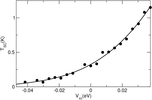
Figure 3: The results of our numerical solution of the linearised gap equations are shown by the points. The line is a fit to the calculated points by a cubic equation.

We now plot the critical temperature for both $\uparrow\uparrow$ and $\downarrow\downarrow$ pairing on the same graph (figure 4). This plot shows is then the ($V_{xc}$, $T$) superconducting phase diagram for our model. (This, of course, assumes that no further phase transitions occur at low temperatures.) The higher transition temperature is the transition to the A₁ phase (where only $\uparrow\uparrow$ pairing occurs) and the second transition is a transition to the A₂ phase (where $\downarrow\downarrow$ pairing begins). In the paramagnetic state (the line $V_{xc}=0$) the superconducting state is an A phase as the superconducting order parameter is the same for both the $\uparrow\uparrow$ and $\downarrow\downarrow$ pairing states. (The A₂ phase becomes the A phase via a cross over, rather than a phase transition.)

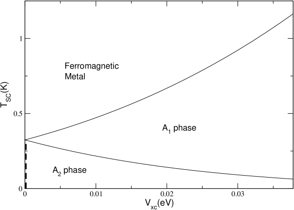
Figure 4: The phase diagram of our model. The critical temperature is shown for both A₁ and A₂ phases over a range of exchange splittings. The hatched area indicates the A phase, which is the ground state when $V_{xc}=0$.

The phase diagram shown in figure 4 is clearly equivalent to the A₁-A₂ splitting of ³He in a magnetic field. Experimental measurement of this phase transition in ³He due to Remeijer et alare reported reference [31]. At first sight figure 4 and reference [31] appear rather different, however the are in fact almost identical, as we will now show. The dimensionless measure of the exchange splitting for the Remijer et alexperiments is $\frac{\mu_{n}B}{k_{B}T_{F}}$, where $T_{F}$ is the Fermi temperature and $\mu_{n}$ is the nuclear magnetron for ³He, while for our calculation the dimensionless exchange splitting is given by $\frac{V_{xc}}{W}$ where $W=16t$ is the bandwidth. The experiments of Remeijer et alwere not performed at constant pressure, which complicates the analysis somewhat, however they conclude that

$$\frac{T_{C}^{A_{1}}-T_{C}^{A_{2}}}{T_{C}^{A}}=\widetilde{a}\left(\frac{\mu_{n}B}{k_{B}T_{F}}\right)+\widetilde{b}\left(\frac{\mu_{n}B}{k_{B}T_{F}}\right)^{2}$$ (145)

where $\widetilde{a}=36.3\pm 0.91$ and $\widetilde{b}=522\pm 17$ in the range $0\leq\frac{\mu_{n}B}{k_{B}T_{F}}\leq 0.01$ at an effective pressure of 3.4 MPa i.e the splitting is, to a very good approximation linear. The equivalent exchange splitting in our calculations is $V_{xc}\leq 0.01\,W=0.01$ eV. It can clearly be seen from figure 4 that our calculations give an approximately linear splitting between the A₁ and A₂ phase transitions over the range of exchange splitting $0\leq V_{xc}\leq 0.01$ eV. Hence our results are consistent with the what is known about ³He. (Although, of course, we had no right to expect this agreement as our parameters where chosen for ZrZn₂ and not ³He.) Further this illustrates the fact that ferromagnetic superconductors will provide an excellent laboratory in which to study the splitting of the A₁ and A₂ phase transitions (and the non-linear splitting in particular) over a far greater range of exchange splitting than is possible in ³He. Further, when the effects of scattering from non-magnetic impurities are included this model gives results that are qualitatively consistent with the observed pressure dependence of $T_{C}$ in ZrZn₂ [16, 30].

5 Discussion

We have derived gap equations for superconductivity in coexistence with ferromagnetism. We have done this for s-wave singlet states and for p-wave triplet states with either ESP or OSP pairing. We used these gap equations to study the behaviour of these states as a function of exchange splitting.

For the singlet state we found that our gap equations reproduced the Clogston–Chandrasekhar limiting behaviour and the phase diagram of the Baltensperger–Sarma equation (neglecting the possibility of an FFLO state). We also showed that the singlet gap equation leads to the result that the superconducting order parameter is independent of exchange splitting at zero temperature. This fact was assumed in the derivation of the Clogston–Chandrasekhar limit.

OSP triplet states showed a very similar behaviour to the singlet state in the presence of exchange splitting. This leads to the conclusion that the effect of exchange splitting on a superconducting state is determined by whether the state contains OSP or ESP. (All singlet states are, by definition, OSP states.)

In contrast, ESP triplet states show a very different behaviour in an exchange field. In particular there is no Clogston–Chandrasekhar limiting. Further, $T_{C}$ is actually increased by exchange splitting because $D_{\sigma}(\varepsilon_{F})$ is changed by the exchange splitting and $T_{C}$ is dependent on $D_{\sigma}(\varepsilon_{F})$. This effect is well known in ³He, but has previously only been studied in a Ginzburg–Landau formalism [32]. The gap equations presented here will allow for far more detailed study of both the increase of $T_{C}$ and for the study of the splitting of the A₁ and A₂ phases by exchange splitting.

If the experimentally occurring ferromagnetic superconductors are ESP triplet pairing states, as seems likely from the absence of Clogston–Chandrasekhar limiting, then these systems will allow for study of this effect at far greater exchange splittings than can be archived with magnetic fields in ³He. The gap equations presented here will also be useful for studying these materials in their own right, in particular we hope that the will prove useful for identifying the superconducting pairing symmetry of these ferromagnetic superconductors. Our formalism is quite general, and can be applied to more realistic band structures and pairing models, although the additional complication of the vector potential will have to be overcome before one can make complete theoretical predictions for these materials.

References

References

• [1] Saxena S S, Agarwal P, Ahilan K, Grosche F M, Haselwimmer R K W, Steiner M J, Pugh E, Walker I R, Julian S R, Monthoux P, Lonzarich G G, Huxley A, Sheikin I, Braithwaite D and Flouquet J 2000 Nature 406 587
• [2] Aoki D, Huxley A, Ressouche E, Braithwaite D, Flouquet J, Brison J-P, Lhotel E and Paulsen C 2001 Nature 413 613
• [3] Pfleiderer C, Uhlarz M, Hayden S M, Vollmer R, von Löhneysen H, Bernhoeft N R and Lonzarich G G 2001 Nature 412 58
• [4] Buzdin A I and Bulaevskii L H 1986 Sov. Phys. Usp. 29 412 (1986 Usp. Fiz. Nauk. 149 45)
• [5] Bulut N, 2002 Adv. Phys. 51 1587
• [6] Eskildsen M R, Harada K, Gammel P L, Abrahamsen A B, Andersen N H, Ernst G, Ramirez A P, Bishop D J, Mortensen K, Naugle D G, Rathnayaka K D D and Canfield P C 1998 Nature 393 242
• [7] Mathur N D, Grosche F M, Julian S R, Walker I R, Freye D M, Haselwimmer R K W and Lonzarich G G 1998 Nature 394 39
• [8] McKenzie R H 1998 Comments Cond. Matt. 18 309
• [9] Fay D and Appel J 1980 Phys. Rev.B 22 3173
• [10] Yates S J C, Santi G, Hayden S M, Meeson P J and Dugdale S B Phys. Rev. Lett. 2003 90 057003
• [11] Cordes H G, Fischer K, and Pobell F 1981 Physica B 107 531
• [12] van Deursen A P J, Schreurs L W M, Admiraal C B, de Boer F R and de Vroomen A R 1986 J. Magn. Mater 54-57 1113
• [13] Balian R and Werthamer N R 1963 Phys. Rev.131 1553
• [14] Vollhardt D and Wölfe P 1990 The Superfluid Phases of Helium 3 (London: Taylor and Francis)
• [15] Powell B J, Annett J F and Györffy B L 2002 Ruthenate and Rutheno-Cuprate Materials: Unconventional Superconductivity, Magnetism and Quantum Phase Transitions (Springer Lecture Notes in Physics vol 603) ed Noce C, Cuoco M, Romano A and Vecchione A (Heidelberg: Springer)
• [16] Powell B J 2002 On the Interplay of Superconductivity and Magnetism Ph.D. thesis, Unversity of Bristol, UK
• [17] Fulde P and Ferrell R A 1964 Phys. Rev.135 A550
• [18] Larkin A I and Ovchinnikov Yu N 1965 Sov. Phys. JETP 20 762
• [19] Mineev V P and Samokhin K V 1999 Introduction to Unconventional Superconductivity (Amsterdam: Gordan and Breach)
• [20] de Gennes P G 1966 Superconductivity of Metals and Alloys (New York: W.A. Benjamin)
• [21] Ketterson J B and Song S N 1999 Superconductivity (Cambridge: Cambridge University Press)
• [22] Györffy B L, Staunton J B and Stocks G M 1991 Phys. Rev.B 44 5190
• [23] Powell B J, Annett J F and Györffy B L The Freedericksz transition in a quasi two dimensional p-wave superconductor Preprint
• [24] Clogston A M 1962 Phys. Rev. Lett.9 266
• [25] Chandrasekhar B S 1962 Appl. Phys. Lett. 1 7
• [26] Zuo F, Brooks J S, McKenzie R H, Schlueter J A and Williams J M 2000 Phys. Rev.B 61 750
• [27] Baltensperger W 1958 Physica 24 S153
• [28] Sarma G 1963 J. Phys. Chem. Solids 24 1029
• [29] Sigrist M and Ueda K 1991 Rev. Mod. Phys.63 239
• [30] Powell B J, Annett J F and Györffy B L Preprint cond-mat/0301364
• [31] Remeijer P, Roobol L P, Steel S C, Jochemsen R and Frossati G 1998 J. Low Temp. Phys. 111 119
• [32] Brussaard P and Capel H W 1999 Physica A 265 370