[

A closer look at symmetry breaking in the collinear phase of the $J_{1}-J_{2}$ Heisenberg Model

Abstract

The large $J_{2}$ limit of the square-lattice $J_{1}-J_{2}$ Heisenberg antiferromagnet is a classic example of order by disorder where quantum fluctuations select a collinear ground state. Here, we use series expansion methods and a meanfield spin-wave theory to study the excitation spectra in this phase and look for a finite temperature Ising-like transition, corresponding to a broken symmetry of the square-lattice, as first proposed by Chandra et al. (Phys. Rev. Lett. 64, 88 (1990)). We find that the spectra reveal the symmetries of the ordered phase. However, we do not find any evidence for a finite temperature phase transition. Based on an effective field theory we argue that the Ising-like transition occurs only at zero temperature.

]

The square-lattice $J_{1}-J_{2}$ Heisenberg antiferromagnet is described by the Hamiltonian

$$H=J_{1}\sum_{{\rm n.n.}}{\bf S}_{i}\cdot{\bf S}_{j}+J_{2}\sum_{{\rm n.n.n.}}{\bf S}_{i}\cdot{\bf S}_{j}$$ (1)

where the first sum runs over the nearest neighbor and the second over the second nearest neighbor spin pairs of the square-lattice. For $J_{1}=0$, the two sublattices are disconnected and individually order antiferromagnetically. For non-zero $J_{1}/J_{2}$ (less than some critical value), in the classical ground state, the two sublattices remain free to rotate with respect to each other. However, quantum fluctuations lift this degeneracy and select a collinear ordered state, where the neighboring spins align ferromagnetically along one axis of the square-lattice and antiferromagnetically along the other [1, 2, 3, 4]. Thus the ground state breaks both spin-rotational symmetry as well as the four-fold symmetry of the square-lattice.

It is well known from the Mermin-Wagner theorem that the continuous spin-rotational symmetry is restored in 2D at any finite temperature. However, the discrete broken lattice symmetry can in principle survive at finite temperatures. In an important paper, Chandra, Coleman and Larkin [2] argued that this symmetry should be restored at a finite temperature phase transition, which lies in the 2D Ising universality class, and gave estimates for the transition temperature. They made use of a linear spin-wave theory (LSWT) for the excitation spectra, which had gapless excitations at four points of the Brillouin zone (($0,0$), ($\pi$,0), (0,$\pi$) and ($\pi,\pi$)).

Recent interest in this model comes from the discovery of two materials Li₂VOSiO₄and Li₂VOGeO₄by Melzi et al. [5, 6]. Electronic structure calculations for these materials [7, 8] lead to $J_{2}$ bigger than $J_{1}$, perhaps by as much as an order of magnitude. The reason for the unusually large $J_{2}$ can be qualitatively understood from the crystal structure. The $VO_{5}$ pyramids alternately point up and down, and hence, the spin-half vanadium atoms are alternately displaced slightly above and slightly below the plane. This causes an increased overlap with the second neighbors which fall in the same plane. Many experimental features of the material are well described by the $J_{1}-J_{2}$ Heisenberg model. However, the value of the ratio $J_{1}/J_{2}$ remains ill-determined [9].

It was argued by Rosner et al. [8] that the measurement of the spin-wave spectra maybe particularly useful for establishing this ratio. One of the purposes of this paper is to present quantitatively accurate spectra for the model going beyond linear spin-wave theory. Indeed, as we will show, the full spectra have gapless excitations at only two symmetry related points of the Brillouin zone (0,0) and (0,$\pi$), whereas the accidental degeneracies at ($\pi,\pi$) and ($\pi,0$) are lifted by the order by disorder effect [1] (here we choose the x axis along the direction of the collinear spin ordering, see Fig. 1). Furthermore, the ratio of the spin-wave velocities along x and y directions depends sharply on the $J_{1}/J_{2}$ ratio and its measurement can indeed be used to determine the latter ratio.

The real materials also have weak interplanar couplings, which eventually lead to 3D long-range order and a finite temperature transition. The specific heat data above the 3D transition does not have any clear features which could be interpreted as a 2D Ising transition. Indeed, the issue of finite-temperature Ising-like transitions may only be relevant to materials with sufficiently weak interplanar couplings. The issue is conceptually important, however. Can long-range Ising order, corresponding to antiferromagnetic correlations along one axis and ferromagnetic correlations along the other, survive at finite temperatures even after the underlying spin-spin correlations become short ranged? That is the somewhat paradoxical prediction of Chandra et al.[2]

We calculate the susceptibility appropriate for this Ising order by high temperature series expansions. The numerical series extrapolations fail to substantiate a finite temperature Ising-like transition, they are only consistent with a $T=0$ phase-transition in a strictly 2D model. We also present field-theoretical arguments in favor of a $T=0$ phase-transition, and find the critical index for the $T=0$ divergence of the susceptibility.

We begin by calculations of the excitation spectra at zero temperature. The standard linear spin-wave theory predicts the dispersion relation[2],

$$\Delta=2J_{2}\left[\left(1+{J_{1}\over 2J_{2}}\cos k_{x}\right)^{2}-\cos^{2}k_{y}\left(\cos k_{x}+{J_{1}\over 2J_{2}}\right)^{2}\right]^{1/2}$$ (2)

and this results in a spectrum with zero modes at four points ${\bf k}=(0,0)$, $(0,\pi)$, $(\pi,\pi)$ and $(\pi,0)$, as discussed by Chandra et al.[2].

We have derived the spin-wave dispersion using a meanfield spin-wave theory (MFSWT), see e.g. Refs. [4, 10]. The result reads

$$\Delta = 2J_{2}\mu{\Big{[}}\left(1+y-\frac{x}{2}(1-\cos k_{x})\right)^{2}$$ (4)

$$-\cos^{2}k_{y}\left(\cos k_{x}+y\right)^{2}{\Big{]}}^{1/2}$$

where $\mu$, $x$ and $y$ are functions of $J_{2}/J_{1}$. For example for

$$J_{2}/J_{1}=2:~{}~{}~{} \mu=1.153,~{}x=0.327,~{}y=0.174$$ (5)

$$J_{2}/J_{1}=1:~{}~{}~{} \mu=1.122,~{}x=0.783,~{}y=0.452$$ (6)

$$J_{2}/J_{1}=0.6:~{} \mu=0.818,~{}x=1.583,~{}y=1.323$$ (7)

This dispersion give a spectrum with zero modes at only two points, i.e. ${\bf k}=(0,0)$ and $(0,\pi)$.

We have performed an Ising expansion[11] of the excitation spectra using the linked-cluster series expansion method, as reviewed recently by Gelfand and Singh [12]. The spin triplet excitation energy $\Delta(k_{x},k_{y})$ has been computed up to order $9$ for the system in the collinear ordered phase. A list of 1796200 linked clusters of up to 10 sites contribute to the triplet excitation spectrum. The series are available on request. Note that the dispersion relation has the symmetry: $\Delta(k_{x},k_{y})=\Delta(k_{x},\pi-k_{y})$.

The excitation spectra for coupling ratios $J_{2}/J_{1}=2,1,0.6$ are shown in Fig. 1, together with those obtained from standard linear spin-wave theory[2] and a MFSWT [10]. We can see from this figure that the spectrum does not have the $90^{\rm o}$ rotational symmetry of the square-lattice. There are zero modes at only two points i.e. ${\bf k}=(0,0)$ and $(0,\pi)$, as predicted by the MFSWT theory, but not the standard theory. In fact, the series expansion data agree with the predictions of the MFSWT theory with remarkable accuracy over the entire range of momenta, except for a small dip in the third panel. The gaps at ${\bf k}=(\pi,\pi)$ and $(\pi,0)$ are non-zero, due to the “order by disorder” effect[1].

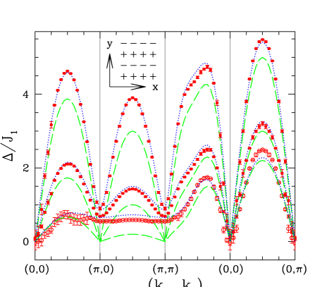
FIG. 1.: Plot of the spin-triplet excitation spectrum $\Delta(k_{x},k_{y})/J_{1}$ along high-symmetry cuts through the Brillouin zone for the system with coupling ratios $J_{2}/J_{1}=2,1,0.6$ shown in the figure from the top to the bottom, respectively; the blue dotted lines are the results of MFSWT, the green dashed lines are the results of LSWT, while the red points with error bar are the results of series expansions. The unperturbed spin configuration assumed in x and y directions are shown as inset.

The gap at ${\bf k}=(\pi,\pi)$ and the spin-wave velocity along $x$ and $y$-directions versus $J_{1}/J_{2}$ are shown in Fig. 2 and Fig. 3. Clearly, the latter anisotropy provides a good way to determine the $J_{1}/J_{2}$ ratio.

FIG. 2.: The spin-triplet excitation gap $\Delta/J_{2}$ at ${\bf k}=(\pi,\pi)$ versus $J_{1}/J_{2}$ obtained from series expansion (the points), and the MFSWT (the solid line).

FIG. 3.: The spin-wave velocity $v/J_{2}$ along x and y-directions versus $J_{1}/J_{2}$ obtained from series expansion (the points with dotted lines connecting them), and the MFSWT (the dashed line).

We now turn to the question of an Ising-like finite temperature transition. To explore the possibility of such a transition we calculate the high temperature series for the susceptibility with respect to the field

$$F=\sum_{i}({\bf S}_{i}\cdot{\bf S}_{i+\hat{x}}-{\bf S}_{i}\cdot{\bf S}_{i+\hat{y}})$$ (8)

i.e. we compute the series for

$$T\chi=\langle F^{2}\rangle-\langle F\rangle^{2}$$ (9)

where

$$\langle Q\rangle={{\rm Tr}Q\exp(-\beta H)\over{\rm Tr}\exp(-\beta H)}$$ (10)

and $\beta=1/(k_{B}T)$; we take $k_{B}=1$ here. Note that $\langle F\rangle$ is zero for the bulk system, but we need to include it in Eq. (9) because it is not zero for each individual cluster in the series expansion.

This field breaks the 90 degree rotational symmetry, as in the zero temperature collinear ordered phase, and if there was a finite temperature transition, one would expect $\chi$ to diverge at the critical temperature. The series has been computed up to order $\beta^{8}$, using the same list of 1796200 linked clusters of up to 10 sites as for the spin dispersion. The series are available on request.

For the full series, we first tried to locate the critical point by Dlog Padé approximants[13], but this did not give any consistent results. We also used integrated differential approximants[13] to extrapolate the series, and the results are shown in Fig. 4. We can see that $1/\chi$ appears to vanish only at zero temperature, rather than at finite temperature. This is consistent also with the results of the Padé approximants. The Ising-like transition temperatures estimated according to [2] are shown in Fig. 4 by arrows.

FIG. 4.: The inverse of susceptibility $1/J_{1}\chi$ versus $T/J_{1}$ for $J_{1}/J_{2}=1,0.25,0.1$. Several different integrated differential approximants to the high-temperature series are shown. The Ising-like transition temperatures estimated according to [2] are shown by arrows.

To look further into this issue, we have also re-analyzed our high-temperature series for the specific heat $C_{v}$[7, 8], for the ratio of couplings in the collinear ordered phase. While the convergence of the series extrapolation is not very good at low temperatures, the Dlog Padé approximants to the series for $C_{v}$ do not show evidence for a finite temperature critical point [9].

We also analyse our numerical results using an effective field theory. The dynamical variables of the problem are two vector fields ${\bf n}_{1}$ and ${\bf n}_{2}$ corresponding to two interpenetrating Neel sublattices with exchange interaction $J_{2}$. Each of the fields is described by the nonlinear $\sigma$-model, and there is also an interaction between the fields. The effective Lagrangian of the system reads [2]

$$L_{\rm eff}=\frac{1}{2}\int d^{2}x\left[\sum_{i=1,2}(\partial_{\mu}{\bf n}_{i})^{2}-g({\bf n}_{1}\cdot{\bf n}_{2})^{2}\right]\ ,$$ (11)

where $g\sim J_{1}^{2}/J_{2}$ is the coupling constant. There are two degenerate energy minima corresponding to $\sigma={\bf n}_{1}\cdot{\bf n}_{2}=\pm 1$. So $\sigma$ imitates an Ising parameter, and at $T=0$ it takes a values corresponding to one of the minima, $\sigma=1$ (x-collinear state) or $\sigma=-1$ (y-collinear state). However, we stress that there is not a dynamical Ising variable in the system, the entire dynamics being described in terms of ${\bf n}_{1}$ and ${\bf n}_{2}$ and the Lagrangian (11). The two minima $\sigma=\pm 1$ are separated by a potential barrier $W(0)\sim EL^{2}$, where $E\sim g$ is the interaction energy density, and $L\to\infty$ is the size of the system.

At a finite temperature, each sublattice behaves as an ordered Neel state up to a length scale $\xi\approx 0.303\exp(2\pi\rho_{s}/T)[1-T/(4\pi\rho_{s})]$, where $\rho_{s}\approx 0.182J_{2}$ is the spin stiffness [14]. At low temperature the energy barrier required to move from the $\sigma=+1$ configuration to the $\sigma=-1$ configuration, $W(T)\sim E\xi^{2}$, remains finite at any finite $T$! So, using the quantum field theory language, one has to say that there is a nontrivial instanton in the problem with tunneling probability $\propto\exp(-E\xi^{2}/T)$. This is different from the true Ising situation, where there is a dynamical Ising field with stiffness, and the tunneling probability $\propto\exp(-E(T)L^{2}/T)\to 0$, as $L\to\infty$. The “true” Ising transition occurs when $E(T)$ vanishes.

Based on the picture described we immediately come to the conclusion that at any finite $T$ the system fluctuates beween $\sigma=1$ and $\sigma=-1$ local minima, and hence the transition temperature for the Ising-like transition is zero in agreement with numerical data. According to this picture one would expect that at low temperature and at $J_{2}>J_{1}$ the suceptibilty with respect to the field (8) behaves as

$$\chi\propto\xi^{\alpha}\propto e^{-1.15\alpha J_{2}/T}\ ,$$ (12)

where $\alpha$ is a critical index, (we neglect the prefactor $[1-T/(4\pi\rho_{s})]$ in $\xi$). Plots of $\ln(J_{1}\chi)$ versus $J_{2}/T$ are presented in Fig. 5. The plots are roughly consistent with prediction (12) with the critical index $\alpha\approx 1$.

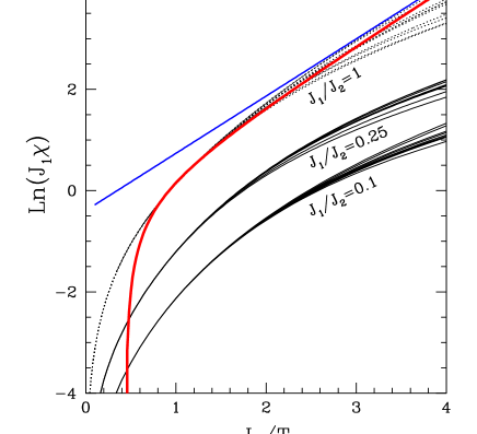
FIG. 5.: $\ln(J_{1}\chi)$ versus $J_{2}/T$ for $J_{1}/J_{2}=1,0.25,0.1$. Also shown are $0.8+\ln\xi$ with (red bold line) and without (blue straight line) the prefactor $[1-T/(4\pi\rho_{s})]$.

In conclusion, in this paper we have studied the collinear phase of the $J_{1}-J_{2}$ square-lattice Heisenberg antiferromagnet by series expansion methods. We have obtained quantitatively accurate excitation spectra, which are significantly more accurate than the spin-wave calculations[2], and should be helpful in determining the exchange parameters for materials with large second neighbor interactions. The MFSWT predicts these spectra with great accuracy. We have also studied an Ising-like phase transition in this model. Using high temperature expansions for the appropriate susceptibility as well as quntum field theory arguments we have shown that the transition temperature is exactly zero.

This work is supported by a grant from the Australian Research Council and by US National Science Foundation grant number DMR-9986948. The computation has been performed on an AlphaServer SC computer. We are grateful for the computing resources provided by the Australian Partnership for Advanced Computing (APAC) National Facility.

REFERENCES

- [1] E.F. Shender, Sov. Phys. JETP 56(1), 1982.
- [2] P. Chandra, P. Coleman and A. I. Larkin, Phys. Rev. Lett. 64, 88 (1990).
- [3] A. V. Chubukov and Th. Jolicoeur, Phys. Rev. B44, 12050 (1991).
- [4] A. F. Barabanov and O. A. Starykh, JETP Lett. 51, 311 (1990).
- [5] R. Melzi, P. Carretta, A. Lascialfari, M. Mambrini, M. Troyer, P. Millet, and F. Mila, Phys. Rev. Lett. 85, 1318 (2000).
- [6] R. Melzi, S. Aldrovandi, F. Tedoldi, P. Carretta, P. Millet, and F. Mila, Phys. Rev. B 64, 024409 (2001).
- [7] H. Rosner, R.R.P. Singh, W. Zheng, J. Oitmaa, S.-L. Drechsler, and W.E. Pickett, Phys. Rev. Lett. 88, 186405 (2002).
- [8] H. Rosner, R. R. P. Singh, W. Zheng, J. Oitmaa, W. E. Pickett, Phys. Rev. B67, 014416, (2003).
- [9] For recent further efforts to deterimne the exchange constants, see G. Misguich, B. Bernu and L. Pierre, cond-mat/0302583.
- [10] See, e.g., A. V. Dotsenko and O. P. Sushkov, Phys. Rev. B 50, 13821 (1994).
- [11] J. Oitmaa and W. Zheng, Phys. Rev. B54, 3022(1996).
- [12] M.P. Gelfand and R.R.P. Singh, Adv. Phys. 49, 93(2000).
- [13] A.J. Guttmann, in “Phase Transitions and Critical Phenomena”, Vol. 13 ed. C. Domb and J. Lebowitz (New York, Academic, 1989).
- [14] S. Chakravarty, B. I. Halperin and D. R. Nelson, Phys. Rev. Lett. 60, 1057 (1988).