A mean-field kinetic lattice gas model of electrochemical cells

Abstract

We develop Electrochemical Mean-Field Kinetic Equations (EMFKE) to simulate electrochemical cells. We start from a microscopic lattice-gas model with charged particles, and build mean-field kinetic equations following the lines of earlier work for neutral particles. We include the Poisson equation to account for the influence of the electric field on ion migration, and oxido-reduction processes on the electrode surfaces to allow for growth and dissolution. We confirm the viability of our approach by simulating (i) the electrochemical equilibrium at flat electrodes, which displays the correct charged double-layer, (ii) the growth kinetics of one-dimensional electrochemical cells during growth and dissolution, and (iii) electrochemical dendrites in two dimensions.

I Introduction

Electrochemical phenomena are ubiquitous in nature and technology. They play a fundamental role in many materials science problems of high practical relevance, such as corrosion, electrodeposition of parts and circuitry, and battery technology BattCorrWeb . Electron transfer is also crucially involved in many biochemical reactions BioElec . For physicists, electrodeposition is interesting because it can lead to the spontaneous formation of highly complex self-organized patterns. Such branched aggregates that are often found on the surfaces of natural minerals have fascinated scientists for centuries because of their plant-like appearance Fleury .

Under well-controlled laboratory conditions, a variety of different patterns can be generated, ranging from compact crystals to highly branched dendritic aggregates that can be fractals (see Figure 1) or densely branched. While dendrites rarely appear in traditional applications of electrodeposition such as metalization and electroplating that take place close to equilibrium, they can be of practical importance far from equilibrium, for example in battery technology Selim74 : Figure 2 shows the growth of dendrites in a lithium battery. Since dendrites can perforate insulating layers and lead to shortcuts when they reach the counterelectrode, they must be eliminated as much as possible. To achieve this goal, a good understanding of the various phenomena occurring in electrochemical cells is necessary. The purpose of our paper is to develop a microscopic model for electrodeposition that can be used to elucidate some of the aspects of dendrite formation.

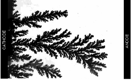
Figure 1: Electrodeposition of copper on a glass substrate (reprinted with permission from V. Fleury). The quasi-two-dimensional cell is made of two copper electrodes and a CuSO₄ solution (sample size $3\times 2\,\mathrm{mm}^{2}$). Only a small part of the sample is shown.

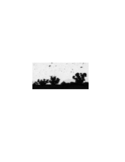
Figure 2: Dendritic growth at the interface between a lithium electrode and a polymer electrolyte (Claire Brissot, PhD thesis, Ecole Polytechnique, Palaiseau, France, 1998)

To fix the ideas, let us consider the simplest possible situation that corresponds to the experimental setup of Figs. 1 and 2: two electrodes made of the same metal are plunged in an electrolyte containing ions of the same metal. When a potential difference is applied by an external generator, as a response an ionic current flows through the electrolyte. Close to the cathode, ions are reduced by electron transfer from the electrode and form a growing deposit. The inverse takes place at the anode: metal is dissolved, and new ions are formed. For liquid electrolytes (such as used in Fig. 1), the inhomogeneities in the ion concentrations lead to strong convective flows Laitinen39 ; Barkey94 ; Huth95 ; Rosso99 . In contrast, for gel-like electrolytes (such as used in Fig. 2), convection is suppressed Rosso94 , and the important ingredients for the description of the ion transport in the electrolyte are diffusion and migration of the ions. At the metal-electrolyte interface, there exists in general a charged double layer that is much thicker than the microscopic solid-electrolyte interface, but much smaller than a typical cell dimension. There is a considerable amount of work on electrochemical cells based on a macroscopic viewpoint Schm in which the microscopic interface is replaced by a mathematically sharp surface. Such models are generally unable to handle the geometrical complexity of a fully developed dendrite. In addition, this approach has to rely on phenomenological models to incorporate reaction kinetics at the interfaces.

In the statistical physics community, considerable interest in electrodeposition was spurned by the fact that the geometrical structure of fractal electrodeposits Matsu84 ; Grier86 ; Sawada86 ; FleuryChaza is strikingly similar to patterns generated by the diffusion-limited aggregation (DLA) model DLA , in which random walkers irreversibly stick to the growing aggregate. Subsequently, many refinements of the DLA model were developed to generate various patterns, for example by the inclusion of surface tension Vicsek84 , anisotropic growth rules and noise reduction Nittmann86 ; Eckmann89 , introduction of a uniform drift to mimic an electric field Meakin83 ; Jullien84 ; Hill97 , and combinations of discrete aggregation and continuous convection models to study the influence of fluid convection Marshall . However, these models greatly simplify the underlying physics (for example, the charged double layers are not included) and can hence not yield detailed information on the relation between growth conditions and characteristics of the growth structures such as growth speed, branch thickness, and overall structure. The same is true for a recent mean-field model that does not explicitly contain the charged ions Elez .

Our goal is to build a simplified microscopic model for electrodeposition that includes enough of the salient physics to make contact with the macroscopic view of electrochemistry. The electrochemical mean-field kinetic equations (EMFKE) developed here are based on a lattice-gas model with simple microscopic evolution rules that contains charged particles, coupled to a discretized version of the Poisson equation. Lattice gas models have been used previously in the context of electrochemistry to simulate phenomena located on the electrode surfaces, such as adsorption or underpotential deposition rikvold0 , and for studies of ionic transport at liquid-liquid interfaces Schm2 ; however, there exists, to our knowledge, no theoretical study of the behavior of an entire electrochemical cell based on a microscopic model.

To investigate the dynamics of the lattice model, we extend the formalism of Mean-Field-Kinetic-Equations (MFKE) Martin90 ; Gouyet93 ; Vaks94 that has been used to study numerous transport and growth phenomena in alloys, including diffusion and ordering kinetics Gouyet95 , spinodal decomposition Dobr96 ; PlappPRL and dendritic growth Plapp ; some preliminary results on the extension to electrochemistry have been published in Refs. Bernard1 ; Bernard2 . The key feature of this approach is that the microscopic particle currents can be written in the mean-field approximation as the product of a mobility times the gradient of chemical potentials, the latter being the appropriate thermodynamic driving forces. The formalism can be generalized in a natural way to charged particles. The driving forces for particle currents are then the gradients of the electrochemical potential. As a consequence, the resulting model displays the correct electrochemical equilibrium at the interfaces. While it obviously still contains strong simplifications, it is much closer to the basic microscopic physics and chemistry than the DLA-type models and allows us to establish a direct link between a microscopic model and the well-established macroscopic phenomenological equations. Quite remarkably, the equations of motion of our model also share many common features with a phase-field formulation of the electrochemical interface that was developed very recently GBW . This indicates that mean-field equations of simplified models can also be useful to understand the connection between phase-field models and a more microscopic viewpoint.

In this paper, we will first present the lattice gas model and derive the electrochemical mean-field kinetic equations (Section 2). In section 3, we carry out one-dimensional simulations to demonstrate that the model leads to the correct equilibrium at the electrode-electrolyte interface. We also calculate one-dimensional steady state solutions for moving interfaces that are in good agreement with the macroscopic continuous model of Chazalviel Chaza90 . Finally, we show some preliminary simulations of dendritic growth in two-dimensional cells. Section 4 contains a brief discussion and conclusion.

II Model

II.1 Lattice gas model

We consider an electrochemical cell made of a dilute binary electrolyte and two metallic electrodes of the same metal. No supporting electrolyte is included in the present study. These conditions correspond to the experimental situation in Figs. 1 and 2 (more precisely, to Fig. 2 since we do not include convection in our model). The electrodes are modeled by a lattice that reflects the underlying crystalline structure, and whose sites are occupied by metallic atoms or vacancies. It is convenient to represent the electrolyte by the same lattice, occupied by a solvent, cations, anions, or vacancies. Although there is no physical lattice in the liquid, its presence here does not play a role due to the high dilution of the ions.

For simplicity, we consider here a two-dimensional lattice gas on a square lattice with lattice spacing $a$ (see Figure 3). The cations $M^{+}$ give metallic atoms $M^{0}$ after reduction, while the anions $A^{-}$ are supposed to be non electroactive. The solvent $S$ is neutral, but can interact through short-range interactions with the other species and with itself. We specify a microscopic configuration by the set $\{n\}$ of the occupation numbers $n_{\mathbf{k}}^{\alpha}$ on each site $\mathbf{k}$: $n_{\mathbf{k}}^{\alpha}=1$ if $\mathbf{k}$ is occupied by species $\alpha=M^{0},M^{+},A^{-},S$ or a vacancy $v$, and $0$ otherwise. We suppose steric exclusion between the different species, that is, a given site can be occupied by only one species or it can be empty (vacancy):

$$\sum_{\alpha}n_{\mathbf{k}}^{\alpha}+n_{\mathbf{k}}^{v}=1\,.$$ (1)

Finally, as will become clear below, it is convenient to introduce electrons in the metallic electrodes. They have a particular status that will be discussed later.

Two very different types of interactions have to be considered. The short-range interactions (including, for example, van der Waals forces, solvatation effects, and chemical interactions) are modeled here by nearest-neighbor interactions $\epsilon^{\alpha\beta}$ between species $\alpha$ and $\beta$ (with the convention that a positive $\epsilon^{\alpha\beta}$ corresponds to an attractive interaction). Interaction energies with vacancies are taken to be zero. To take into account the long-range electrostatic interaction, it would be possible to introduce appropriate interaction energies with farther neighbors; however, this procedure becomes cumbersome with increasing interaction range. Instead, we consider a “coarse-grained” electrical potential $V_{\mathbf{k}}$ defined on the lattice sites $\mathbf{k}$ (that is, a potential that has been smoothed over distances smaller than $a$) and that obeys Poisson’s equation with the simplest nearest-neighbor discretization for the Laplace operator,

$$\sum_{\mathbf{a}}V_{\mathbf{k+a}}-4V_{\mathbf{k}}=-\frac{a^{2-d}}{\epsilon}\sum_{\alpha=+,-}q^{\alpha}n_{\mathbf{k}}^{\alpha}$$ (2)

where $\epsilon$ is the dielectric constant (for simplicity, we take a constant that is the same for all species), $q^{\alpha}$ is the electric charge of species $\alpha$, and $d$ the spatial dimension. This equation has to be solved in the electrolyte, that is, outside of the metal clusters connected to the ends of the cell, and subject to the boundary condition of constant potential in each electrode.

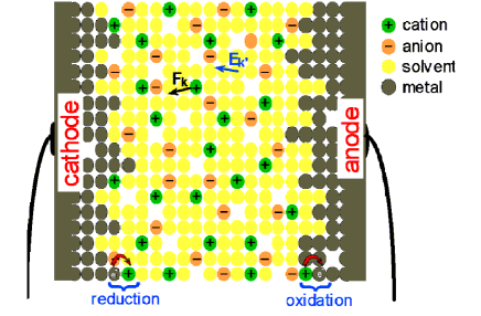
Figure 3: The lattice gas model. A fixed potential difference is applied across the cell. The ions in the electrolyte are submitted to an electric field $\mathbf{E}_{\mathbf{k}}$ (and hence a force $\mathbf{F}_{\mathbf{k}}=q\mathbf{E}_{\mathbf{k}}$) at their lattice site position $\mathbf{k}$. The various species have short range interactions (here, attractive interactions are considered between solvent and ions, solvent and solvent, and metal and metal). Electron transfer takes place on the electrode surfaces.

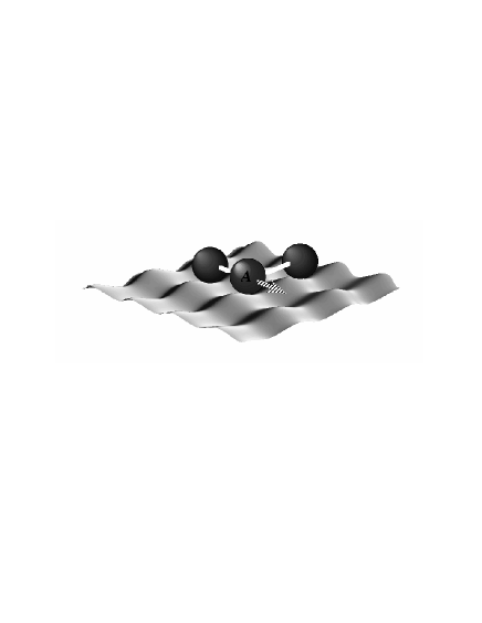
Figure 4: In the lattice gas model, an A atom makes activated jumps to empty nearest neighbor sites. The barrier it has to overcome depends on its interactions (white links) with its nearest neighbor atoms.

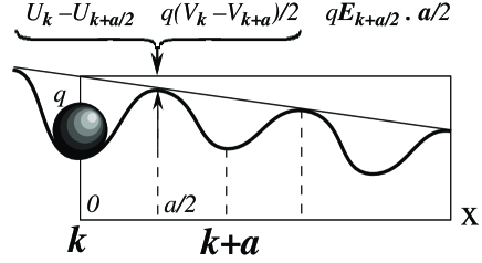
Figure 5: In presence of an electric field $\mathbf{E}$, a potential energy which varies, to first order, like $q\mathbf{E}.\mathbf{x}$ along the jump path $\mathbf{x}$, is superimposed to the local potential seen by a moving particle (with charge $q$).

The configurations evolve when one particle (metal, ion, or solvent) jumps to one of its vacant nearest neighbor sites. In principle, we could also include an exchange process between occupied nearest neighbor sites. This leads to more complicated kinetic equations and has not been considered here. To specify the jump rates, we assume that the atoms perform activated jumps. The height of the activation barrier depends on the local binding energy, that is, the number and type of bonds that need to be broken (see Fig. 4), and, for charged particles, on the local electric field that shifts the barrier height as shown in Fig. 5. The result for the jump rate from site $\mathbf{k}$ to site $\mathbf{k+a}$ is

$$\widetilde{w}_{\mathbf{k,k+a}}^{\alpha}(\{n\}) = w^{\alpha}\exp\left(-\frac{1}{kT}\sum_{\beta}\sum_{\mathbf{a^{\prime}}}\epsilon^{\alpha\beta}n_{\mathbf{k+a^{\prime}}}^{\beta}\right)$$ (3)

$$\quad\mbox{}\times\exp\left(\frac{q^{\alpha}}{2kT}(V_{\mathbf{\ k}}-V_{\mathbf{k+a^{\prime}}})\right),$$

where $kT$ is the (fixed) thermal energy, and $w^{\alpha}$ is a fixed jump frequency that may be different for each species. Here and in the following, symbols with tildes will denote electrochemical quantities that are sensitive to the electric potential.

II.2 Mean-field kinetic equations

The derivation of the Electrochemical Mean-Field Kinetic Equations (EMFKE) follows the same procedure as for neutral particles Martin90 ; Gouyet93 ; Vaks94 . We first write the Boolean kinetic equations on the lattice, starting from the general master equation,

$$\frac{\partial}{\partial t}P(\{n\},t) = \sum_{\{n^{\prime}\}}\left[W(\{n^{\prime}\}\rightarrow\{n\})P(\{n^{\prime}\},t)\right.$$ (4)

$$\quad\left.\mbox{}-W(\{n\}\rightarrow\{n^{\prime}\})P(\{n\},t)\right]$$

which gives the probability $P$ to find a given configuration $\{n\}$ at time $t$. $W(\{n\}\rightarrow\{n^{\prime}\})$ is the rate of evolution from configuration $\{n\}$ to configuration $\{n^{\prime}\}$. We are interested in the time evolution of the average concentrations of the various species ($\alpha=+,-,0,S,v)$,

$$p_{\mathbf{k}}^{\alpha}(t)=\left\langle n_{\mathbf{k}}^{\alpha}\right\rangle_{t}=\sum_{\{n\}}n_{\mathbf{k}}^{\alpha}P(\{n\},t).$$ (5)

In the absence of electrochemical processes at the electrodes, the number of each type of particles remains constant, and the kinetic equation of the average concentration has the structure of a conservation equation,

$$\frac{\partial p_{\mathbf{k}}^{\alpha}}{\partial t}=-\sum_{\mathbf{a}}\widetilde{J}_{\mathbf{k,k+a}}^{\alpha},$$ (6)

with the current of species $\alpha$ on link $\{\mathbf{k,k+a\}}$ defined by,

$$\widetilde{J}_{\mathbf{k,k+a}}^{\alpha}=\left\langle\widetilde{w}_{\mathbf{k,k+a}}^{\alpha}(\{n\})n_{\mathbf{k}}^{\alpha}n_{\mathbf{k+a}}^{v}-\widetilde{w}_{\mathbf{k+a,k}}^{\alpha}(\{n\})n_{\mathbf{k+a}}^{\alpha}n_{\mathbf{k}}^{v}\right\rangle,$$ (7)

with $\widetilde{w}_{\mathbf{k,k+a}}^{\alpha}(\{n\})$ given by Eq. (3). The factor $n_{\mathbf{k}}^{\alpha}n_{\mathbf{k+a}}^{v}$ (and $n_{\mathbf{k+a}}^{\alpha}n_{\mathbf{k}}^{v}$ for the reverse jump) means that for a jump of $\alpha$ to be possible, the start site must be occupied by species $\alpha$, while the target site must be empty (occupied by a vacancy $v$).

In the mean-field approximation, the occupation numbers $n_{\mathbf{k}}^{\alpha}$ in the above expressions are replaced by their average $p_{\mathbf{k}}^{\alpha}$. This replacement is not unique because of different possible choices for the factorization of the occupation number operators Gouyet93 . A convenient choice Gouyet93 ; Plapp is the direct replacement of all occupation numbers by their averages in Eqs. (7) and (3), which leads to

$$\widetilde{J}_{\mathbf{k,k+a}}^{\alpha} = w^{\alpha}\Biggl{[}p_{\mathbf{k}}^{\alpha}p_{\mathbf{k+a}}^{v}\exp\Bigr{(}-\frac{1}{kT}\sum_{\beta}\sum_{\mathbf{a^{\prime}}}\epsilon^{\alpha\beta}p_{\mathbf{k+a^{\prime}}}^{\beta}$$ (8)

$$\qquad\qquad\qquad\mbox{}+\frac{q^{\alpha}}{2kT}(V_{\mathbf{k}}-V_{\mathbf{k+a}})\Bigr{)}$$

$$\mbox{}-p_{\mathbf{k+a}}^{\alpha}p_{\mathbf{k}}^{v}\exp\Bigl{(}-\frac{1}{kT}\sum_{\beta}\sum_{\mathbf{a^{\prime}}}\epsilon^{\alpha\beta}p_{\mathbf{k+a+a^{\prime}}}^{\beta}$$

$$\qquad\qquad\qquad\mbox{}+\frac{q^{\alpha}}{2kT}(V_{\mathbf{k+a}}-V_{\mathbf{k}})\Bigr{)}\Biggr{]}.$$

This expression can be rewritten without any further approximation as the product of an electrochemical bond mobility $\widetilde{M}_{\mathbf{ij}}^{\alpha}$ times the (discrete) gradient of an electrochemical potential $\widetilde{\mu}_{\mathbf{i}}^{\alpha}$,

$$\widetilde{J}_{\mathbf{k,k+a}}^{\alpha}=-\widetilde{M}_{\mathbf{k,k+a}}^{\alpha}\mathfrak{D}_{\mathbf{a}}\widetilde{\mu}_{\mathbf{k}}^{\alpha},$$ (9)

where $\mathfrak{D}_{\mathbf{a}}$ is a difference operator acting on the site coordinates, $\mathfrak{D}_{\mathbf{a}}f_{\mathbf{k}}=f_{\mathbf{k+a}}-f_{\mathbf{k}}$. The electrochemical potential,

$$\widetilde{\mu}_{\mathbf{k}}^{\alpha} = \mu_{\mathbf{k}}^{\alpha}+q^{\alpha}V_{\mathbf{k}}$$ (10)

$$= -\sum_{\beta}\sum_{\mathbf{a}}\varepsilon^{\alpha\beta}p_{\mathbf{k+a}}^{\beta}+kT\ln\left(\frac{p_{\mathbf{k}}^{\alpha}}{p_{\mathbf{k}}^{v}}\right)+q^{\alpha}V_{\mathbf{k}},$$

is the sum of three contributions, a local energy due to the interaction of species $\alpha$ with its local environment, an entropy term (these two constitute the chemical potential $\mu_{\mathbf{k}}^{\alpha}$), and an electrostatic energy $q^{\alpha}V_{\mathbf{k}}$. The presence of the vacancy concentration in the denominator of the entropic contributions comes from the constraint of Eq. (1). The mobility along a bond $\mathbf{i}$ -$\mathbf{j}$ is given by

$$\widetilde{M}_{\mathbf{k,k+a}}^{\alpha}=\frac{w^{\alpha}}{kT}p_{\mathbf{k}}^{v}p_{\mathbf{k+a}}^{v}\exp\frac{(\widetilde{\mu}_{\mathbf{k}}^{\alpha}+\widetilde{\mu}_{\mathbf{k+a}}^{\alpha})}{2kT}\mathrm{shc}\frac{\mathfrak{D}_{\mathbf{a}}\widetilde{\mu}_{\mathbf{k}}^{\alpha}}{2kT},$$ (11)

where we have used the notation $\mathrm{shc~{}}u=\sinh u/u$ (close to equilibrium, $\widetilde{\mu}_{\mathbf{k+a}}^{\alpha}\cong\widetilde{\mu}_{\mathbf{k}}^{\alpha}$ and $\mathrm{shc}\left[\mathfrak{D}_{\mathbf{a}}\widetilde{\mu}_{\mathbf{k}}^{\alpha}/2kT\right]\cong 1$ ).

In a dilute electrolyte, where the concentration of species $\alpha=+,-,0,$ and $v$ is low, neglecting all the terms of order larger than two in the concentrations and discrete gradients, the current $\widetilde{J}_{\mathbf{k,k+a}}^{\alpha}$ simplifies,

$$\widetilde{J}_{\mathbf{k,k+a}}^{\alpha}=-w_{\mathbf{k}}^{\alpha}\left(\mathfrak{D}_{\mathbf{a}}p_{\mathbf{k}}^{\alpha}+\frac{p_{\mathbf{k}}^{\alpha}}{p_{\mathbf{k}}^{v}}\mathfrak{D}_{\mathbf{a}}p_{\mathbf{k}}^{v}+\frac{q^{\alpha}}{kT}p_{\mathbf{k}}^{\alpha}\mathfrak{D}_{\mathbf{a}}V_{\mathbf{k}}\right),$$ (12)

where $w_{\mathbf{k}}^{\alpha}=w_{0}^{\alpha}\exp\left(-(1/kT)\sum_{\beta}\sum_{\mathbf{a^{\prime}}}\epsilon^{\alpha\beta}p_{\mathbf{\ k+a^{\prime}}}^{\beta}\right)$. This is the discrete form of the continuous macroscopic expression

$$\mathbf{j}^{\alpha}=-D^{\alpha\alpha}\mathbf{grad~{}}c^{\alpha}-D^{\alpha v}\mathbf{grad~{}}c^{v}+D^{\alpha\alpha}\frac{q}{kT}c\mathbf{E},$$ (13)

with a concentration-dependent diffusion coefficient $D^{\alpha\alpha}=a^{2}w^{\alpha}$, an off-diagonal diffusion coefficient $D^{\alpha v}=a^{2}w^{\alpha}c^{\alpha}/c^{v}$ associated with the gradient of the vacancy concentration, and the correspondence between a $d$-dimensional cubic lattice and the $d-$dimensional continuous space $J_{\mathbf{k,k+a}}\Rightarrow a^{d-1}\mathbf{j},p_{\mathbf{k}}\Rightarrow a^{d}c$. When the vacancy concentration is homogeneous, the off-diagonal term is absent, and Eq. (13) is exactly the classical continuous description of ion diffusion and migration.

So far, the mean-field equations are quite similar to the ones governing the evolution of multi-component alloys. However, two important new elements have now to be taken into account: (i) how to calculate the electric potential in the mean-field model, and (ii) the electrochemical reactions at the electrodes.

II.3 The Poisson problem

The electric potential has to be obtained, as before, by resolving Poisson’s equation. However, some additional considerations are necessary, because it turns out that the treatment of the boundary conditions at the electrode surfaces becomes non-trivial in the mean-field context. To understand this, it is useful to start with some comments on the consequences of the mean-field approximation. The parameters of the model that control the phase diagram are the various interaction energies and the temperature. Obviously, we want to create and maintain two distinct phases, namely the metallic electrodes and the electrolyte. Hence, the interaction energies need to be chosen such that phase separation occurs. As usual for this kind of lattice models, there exists a critical temperature for phase separation. Close below the critical point, the equilibrium concentrations of the two phases are close to each other, that is, there are many metal particles in the electrolyte phase, and vice versa. The concentration of these minority species decreases with temperature. In the original lattice gas model, it is then possible for low enough temperatures to identify the geometry of the bulk phases with the connected clusters of metal and electrolyte species.

In the mean-field approximation, the concentration variables (occupation probabilities) are continuous, and each species has a non-vanishing concentration at each site. This means that the electrode always contains small quantities of solvent and ions, and the electrolyte contains a small quantity of metal. Of course, these concentrations can be made arbitrarily small by lowering the temperature. However, we then face another difficulty. The interface between the two bulk phases, which was the sharp boundary between connected clusters in the discrete model, is now diffuse with a characteristic thickness that depends on the temperature. For low temperatures, this thickness becomes smaller than the lattice spacing, which leads to strong lattice effects on static and dynamic properties of the interface Cahn60 ; Kessler90 ; Plapp97b : the surface tension and mobility of the interface depend on its position and orientation with respect to the lattice, and for very low temperatures the interface can be entirely pinned in certain directions. As a consequence, we have to make a compromise in choosing the temperature: it must be low enough to obtain reasonably low concentrations of the minority species, but high enough to avoid lattice pinning and to obtain a reasonably diffuse interface (that extends over a few lattice sites).

This has consequences for the resolution of Poisson’s equation. The boundary conditions of constant electric potential in the electrodes are easy to impose in a model with sharp boundaries. For diffuse interfaces, we have to decide where the electrodes end. Another way to state the problem is to remark that the existence of an electric field in the electrolyte creates surface charges in the conductor that are localized at the surface. In a system with diffuse interfaces, this surface charge is “smeared out” over the thickness of the interface, and we need a method to determine this charge distribution.

We solve these problems by the introduction of electrons that are free to move within the metallic electrodes and solve the Poisson equation for all the charges, including electrons. More precisely, we denote by $p_{\mathbf{k}}^{e}$ the deviation from the neutral state expressed in electrons per site. Hence, $p_{\mathbf{k}}^{e}>0$ corresponds to an excess of electrons, $p_{\mathbf{k}}^{e}<0$ to an electron deficit. Their chemical potential is defined by

$$\widetilde{\mu}_{\mathbf{k}}^{e}=E_{F}+q^{e}V_{\mathbf{k}}+\frac{p_{\mathbf{k}}^{e}}{\mathcal{D}(E_{F})},$$ (14)

$\mathcal{D}(E_{F})$ being the density of electronic states at the Fermi level $E_{F}$ of the metal, and $q^{e}=-e$. This corresponds to the screening approximation of Thomas-Fermi Chaz . The electronic current is then written as an electronic mobility times the discrete gradient of the chemical potential,

$$\widetilde{J}_{\mathbf{k,k+a}}^{e}=-\widetilde{M}_{\mathbf{k,k+a}}^{e}\mathfrak{D}_{\mathbf{a}}\widetilde{\mu}_{\mathbf{k}}^{e},$$ (15)

and the time evolution of the excess electron concentration is

$$\frac{\partial p_{\mathbf{k}}^{e}}{\partial t}=-\sum_{\mathbf{a}}\widetilde{J}_{\mathbf{k,k+a}}^{e}.$$ (16)

Note that the choice of this dynamics is somewhat arbitrary; it could be replaced by any other process that leads to an equilibrium of the electron distribution with the ionic charge distribution on a time scale that is much faster than the characteristic time of evolution of the other species.

One important feature is that the electrons must remain in the electrodes; otherwise, a “leakage” current may occur. We have tested two different possibilities to achieve this goal. We can either consider that the electrons are in a potential well in the metallic regions such that they remain confined in the metal, or we can suppose that their mobility vanishes outside the metallic regions. Here, we have chosen the second possibility and written the mobility in the form,

$$\widetilde{M}_{\mathbf{k,k+a}}^{e}=\frac{w^{e}}{kT}f(p_{\mathbf{k}}^{0})f(p_{\mathbf{k+a}}^{0}),$$ (17)

where $w^{e}$ is a constant frequency prefactor, and $f$ is an interpolation function that is equal to $1$ for large metal concentrations and falls to zero for low metal concentrations. With this choice, the electronic jump probability is important only if nearest neighbor sites $\mathbf{k}$ and $\mathbf{k+a}$ have a large enough probability to be occupied by metallic atoms. We have used for $f$

$$f(p)=\frac{\tanh[(p-p_{c})/\xi]+\tanh[p_{c}/\xi]}{\tanh[(1-p_{c})/\xi]+\tanh[p_{c}/\xi]},$$ (18)

a monotonous function that varies from $0$ when $p=0$ to $1$ for $p=1$, with a rapid increase through an interval in $p$ of order $\xi$ centered around some concentration $p_{c}$ that is reminiscent of a percolation threshold. This interpolation is motivated by the fact that the metallic region must be dense enough to be connected and thus allow the electrons to propagate.

To determine the electrostatic potential, we solve the mean-field version of Poisson’s equation, including the new contribution from the electrons,

$$\sum_{\mathbf{a}}V_{\mathbf{k+a}}-4V_{\mathbf{k}}=-\frac{a^{2-d}}{\epsilon}\sum_{\alpha=+,-,e}q^{\alpha}p_{\mathbf{k}}^{\alpha}.$$ (19)

This equation is now solved in the whole system, including the electrodes. Note that we still use a constant permittivity $\epsilon$; however, the phase-dependent mobility of the electrons makes the resistivity in the electrolyte much higher than in the metal.

This method provides a fast way to calculate the surface charges on the electrodes. As will be shown below, it works perfectly well at equilibrium. However, in out-of-equilibrium simulations, a problem appears on the side of the anode where the metal is dissolved. Since the mobility rapidly decreases with the metal concentration, electrons present on the metallic site before dissolution may be trapped in the electrolyte, leading to spurious electronic charges in the bulk. We have solved this problem in a phenomenological way by adding a term to the evolution equation for the electrons that relaxes the electronic charge to zero in the electrolyte,

$$\frac{\partial p_{\mathbf{k}}^{e}}{\partial t}=-\sum_{\mathbf{a}}\widetilde{J}_{\mathbf{k,k+a}}^{e}-w^{e}[1-f_{r}(p_{\mathbf{k}}^{0})]p_{\mathbf{k}}^{e},$$ (20)

where $f_{r}(p^{0})$ is the same interpolation function as $f$, but with different parameters $\xi_{r}$ and $p_{c,r}$. With a convenient choice of these parameters, “electron relaxation” occurs only in the liquid.

II.4 Electron transfer

On the electrode surfaces, electron transfer takes places. More precisely, metallic cations $M^{+}$ located in the electrolyte may receive an electron from a neighboring metallic site and be reduced; in turn, metal atoms in contact with the electrolyte may reject an electron to a neighboring metallic site and become an ion,

$$M^{+}(\mathbf{k)}+e^{-}(\mathbf{k+a)}\rightleftharpoons M^{0}(\mathbf{k)}.$$ (21)

The direction of the transfer depends on the relative magnitude of the electrochemical potentials of the involved species. Reduction of cations on a site $\mathbf{k}$ of the cathode appears when

$$\widetilde{\mu}_{\mathbf{k}}^{+}+\widetilde{\mu}_{\mathbf{k+a}}^{e}>\widetilde{\mu}_{\mathbf{k}}^{0},$$ (22)

otherwise, the metal is oxidized. Consequently, we define $\sigma_{\mathbf{k,k+a}}$ as the current of electronic charges from $\mathbf{k+a}$ to $\mathbf{k}$ (current of positive charges from $\mathbf{k}$ to $\mathbf{k+a}$ ) reducing the cations on site $\mathbf{k}$ (resp. electronic current issued from the oxidation of the metal) via a corresponding elimination (resp. creation) of electrons on site $\mathbf{k+a}$. Following Schm , we can write the reaction rate,

$$\sigma_{\mathbf{k,k+a}}=w_{\mathbf{k,k+a}}^{*}\left(\exp\frac{\widetilde{\mu}_{\mathbf{k}}^{+}+\widetilde{\mu}_{\mathbf{k+a}}^{e}}{kT}-\exp\frac{\widetilde{\mu}_{\mathbf{k}}^{0}}{kT}\right).$$ (23)

This corresponds to an activated electronic charge transfer between the metal surface and the nearest neighboring cation. The total reduction rate on site $\mathbf{k}$ is the sum of all the reaction paths $\sum_{\mathbf{a}}\sigma_{\mathbf{k,k+a}}$. The coefficient $w_{\mathbf{k,k+a}}^{*}$ can be determined by comparison with the mesoscopic theory of Butler-Volmer (see the Appendix).

The currents $\sigma_{\mathbf{k,k+a}}$ have non negligible values only on the interfaces. However, as discussed before, there are small concentrations of ions in the metal and metal atoms in the electrolyte; this would lead to undesirable contributions of the reaction term inside the bulk phases. Therefore, we use the same interpolation function $f(p)$ as for the electron mobility and write

$$w_{\mathbf{k,k+a}}^{*}=w^{*}\left(1-f(p_{\mathbf{k}}^{0})\right)f(p_{\mathbf{k+a}}^{0})\;,$$ (24)

where $w^{*}$ is again a constant frequency factor. In this way, the transfer is localized around the metal-electrolyte interface, where occupied metallic sites and electrolyte sites are neighbors. To completely suppress the electrochemical processes in the bulk phases, we set the transfer current to zero when the product of the two interpolation prefactors is smaller than $10^{-4}$.

II.5 Summary

After all the different pieces are combined, the complete set of equations is

$$\frac{\partial p_{\mathbf{k}}^{+}}{\partial t}=-\sum_{\mathbf{a}}\widetilde{J}_{\mathbf{k,k+a}}^{+}-\sum_{\mathbf{a}}\sigma_{\mathbf{k,k+a}},$$ (25)

$$\frac{\partial p_{\mathbf{k}}^{0}}{\partial t}=-\sum_{\mathbf{a}}\widetilde{J}_{\mathbf{k,k+a}}^{0}+\sum_{\mathbf{a}}\sigma_{\mathbf{k,k+a}},$$ (26)

$$\frac{\partial p_{\mathbf{k}}^{-}}{\partial t}=-\sum_{\mathbf{a}}\widetilde{J}_{\mathbf{k,k+a}}^{-},$$ (27)

$$\frac{\partial p_{\mathbf{k}}^{s}}{\partial t}=-\sum_{\mathbf{a}}\widetilde{J}_{\mathbf{k,k+a}}^{s},$$ (28)

$$\frac{\partial p_{\mathbf{k}}^{e}}{\partial t}=-\sum_{\mathbf{a}}\widetilde{J}_{\mathbf{k,k+a}}^{e}-w^{e}[1-f_{r}(p_{\mathbf{k}}^{0})]p_{\mathbf{k}}^{e}-\sum_{\mathbf{a}}\sigma_{\mathbf{k+a,k}},$$ (29)

$$\sum_{\mathbf{a}}V_{\mathbf{k+a}}-4V_{\mathbf{k}}=-\frac{a^{2-d}}{\epsilon}\sum_{\alpha=+,-,e}q^{\alpha}p_{\mathbf{k}}^{\alpha}.$$ (30)

The local concentration of the species $M^{0}$ and $M^{+}$ is modified by transport (diffusion and migration in the electric field) and by the chemical reaction; for the other species $A^{-}$ and $S$, only transport is present. The reaction term is active only in the solid-electrolyte interface and has of course an opposite sign in Eqs. (25) and (26), and no contributions in Eqs. (27) and (28).

Equations (25) through (29) are integrated in time by a simple Euler scheme (with constant or variable timestep). Two methods are used to solve Poisson’s equation. Equation (30) can either be solved for each timestep using a conjugate gradient method, or it can be converted into a diffusion equation with a source term and solved by simple relaxation; the second method generally is computationally faster and converges well for interfaces that move slowly enough.

III Numerical tests

III.1 Chemical equilibrium

The complete EMFKE model involves a considerable number of parameters. In particular, we need to make a choice for all the short-range interaction energies. They determine the phase diagram of the four-component system that consists of metal, solvent, anions, and cations. To obtain meaningful results, the model has to be used not too far from a two-phase equilibrium between a metal-rich electrode and a liquid phase rich in solvent and ions. For an arbitrary choice of interaction energies, obtaining the equilibrium concentrations for all of the species in the two phases is not a trivial task. The conditions for a two-phase equilibrium are (i) equal electrochemical potentials for each independent species (four in our case), and (ii) equal grand potential. This yields five conditions for eight unknowns (four equilibrium concentrations in each phase); consequently, three degrees of freedom remain that may be fixed, for example the concentrations of ions and metal in the liquid. This constitutes a set of five coupled nonlinear equations for the remaining unknowns.

To simplify the task of finding an equilibrium configuration, we start from a simpler system, namely a mixture of metal, solvent, and vacancies, that is equivalent to a binary alloy with vacancies (ABv). For a symmetric interaction matrix, $\epsilon^{00}=\epsilon^{ss}$, the phase diagram can be determined analytically PlappPRL . A two-phase equilibrium exists with $p^{s}_{liq}=p^{0}_{sol}$ and $p^{0}_{liq}=p^{s}_{sol}$. The equilibrium concentrations can be expressed in terms of the new variables $P=p^{s}_{liq}+p^{0}_{liq}=p^{s}_{sol}+p^{0}_{sol}$ and $Q=p^{s}_{liq}-p^{0}_{liq}=p^{0}_{sol}-p^{s}_{sol}$ and the reduced interaction energy $\bar{\epsilon}=(\epsilon^{00}+\epsilon^{ss}-2\epsilon^{0s})/2$ as

$$P=Q/\tanh\left(\frac{z\bar{\epsilon}Q}{2kT}\right),$$ (31)

where $z$ is the coordination number ($z=4$ for a square lattice in two dimensions). For the rest of the section, we choose $\epsilon^{00}/kT=\epsilon^{ss}/kT=1$, $\epsilon^{0s}=0$, and $Q=0.9$, which gives $p^{s}_{liq}=p^{0}_{sol}=0.92528$, $p^{0}_{liq}=p^{s}_{sol}=0.02528$, and $p^{v}_{liq}=p^{v}_{sol}=0.04944$.

Next, this equilibrium is perturbed by the addition of ions. If the interaction energies are taken identical for both species of ions, no separation of charge occurs at equilibrium and in the absence of an applied voltage, and we can for the moment omit the Poisson equation. We take $\epsilon^{+s}/kT=\epsilon^{-s}/kT=1$ and $\epsilon^{++}=\epsilon^{--}=\epsilon^{+0}=\epsilon^{-0}=0$. This means that the ions are attracted by the solvent, and that the energy density of the liquid does not change upon addition of ions. As long as the equilibria of the main components are not appreciably modified, we expect an equilibrium distribution of the ions that satisfies

$${\frac{p^{\pm}_{sol}}{p^{\pm}_{liq}}}=\exp\left(-{\frac{z\epsilon^{\pm s}Q}{kT}}\right).$$ (32)

We tested this prediction by performing simulations of one-dimensional half cells of length 40, in which 20 lattice sites of solid are in contact with 20 lattice sites of liquid. In each phase, all concentration values are initially set to the expected equilibrium values. On the solid side, we apply no-flux boundary conditions, whereas at the liquid side the concentrations are kept constant. This corresponds to a finite-size isolated electrode plunged in an infinite solution. The electrochemical reaction is suppressed by setting $w^{\star}=0$; all other frequency factors $w^{\alpha}$ are set to $1$. The equations are integrated with a fixed timestep of $\Delta t=1$.

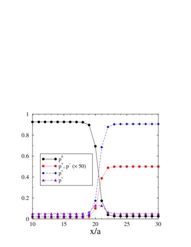
Figure 6: Concentration profiles obtained from the relaxation of a step profile (20 sites of solid in contact with 20 sites of electrolyte) with ion concentration in the liquid of $p^{\pm}_{liq}=0.01$. The other parameters are given in the text.

Figure 7: Ion concentration in the solid $p^{\pm}_{sol}$ in equilibrium with a liquid of fixed ion content $p^{\pm}_{liq}$.

Two ways of adding ions were tested. In the first case, $p^{v}_{liq}$ is kept constant and a small percentage of solvent is replaced by ions. Within a few $10^{6}$ timesteps, the chemical potential differences across the cell fall below $10^{-9}$ and the evolution virtually stops. The concentration profiles obtained for $p^{+}_{liq}=p^{-}_{liq}=0.01$ are shown in Fig. 6. In Fig. 7, we plot the ion concentration in the solid versus the ion concentration in the liquid. For low concentrations, Eq. (32) is well satisfied. For concentrations larger than $\approx 10^{-3}$, deviations appear because the concentrations of metal, solvent and vacancies are shifted. However, even for $p^{\pm}_{liq}=0.01$ this deviation is less than 5%.

In the second case, ions were added in replacement of vacancies ($p^{s}_{liq}$ and $p^{0}_{liq}$ were kept constant). Here, the solvent-metal equilibrium is shifted more rapidly due to the strong dependence of the chemical potentials on the vacancy concentration. For ion concentrations larger than $0.003$, the interface never relaxes, but starts to grow by incorporating metal that is transported to the interface from the solution by chemical diffusion. Of course, the fact that the system does not reach equilibrium is due to the fact that we have fixed one degree of freedom too much, namely all four concentrations in the liquid. Consequently, even the solutions found by the first method are not, strictly speaking, equilibrium solutions; however, they are sufficiently close to equilibrium for all practical purposes and will hence be used as initial conditions in the following.

III.2 Poisson equation and screening: perfectly polarizable electrode

To test our method for creating interface charges, we started from an equilibrated half cell as calculated in the preceding subsection, added a potential difference between electrode and solution, and opened the metal side of the cell for a current of electrons (but not of other species). Since the electron transfer frequency was kept to zero ($w^{\star}=0$), and hence no electrochemical processes can take place, this situation corresponds to a grounded perfectly polarizable electrode.

For simplicity, we have restricted our attention here to the case of monovalent ions ($q^{+}=e$, $q^{-}=-e$). In our tests, we want the thickness of the charged double layer to be a few lattice constants. This can be achieved by choosing the dielectric constant $\epsilon=0.05e^{2}/(akT)$. Furthermore, we choose for the density of states at the Fermi level ${\mathcal{D}(E_{F})}=1000/kT$. Since $kT{\mathcal{D}(E_{F})}\gg 1$, the electrochemical potential of the electrons depends only weakly on the surface charge. The parameters of the interpolation functions are fixed to $p_{c}=0.5$, $\xi=0.1$ for the electron mobility (this leads to an electron mobility that is 8 orders of magnitude smaller in the liquid than in the electrodes) and $p_{c,r}=0.03$, $\xi_{r}=0.001$ for the electron relaxation (see Eq. (20); this corresponds to an interpolation function with a sharp increase at a concentration slightly larger than the equilibrium metal concentration in the liquid). The resulting interface profile for $p^{\pm}_{liq}=0.01$ and a potential difference of $\Delta V=V_{metal}-V_{liquid}=-0.5kT/e$ is plotted in Fig. 8. As expected, the cations are attracted to the electrode, whereas the anions are repelled.

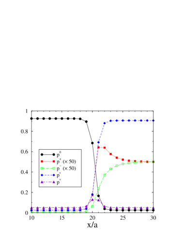
Figure 8: Concentration profiles with the same parameters as in Fig. 6, but with a potential difference $\Delta V=-0.5kT/e$ between metal and solution.

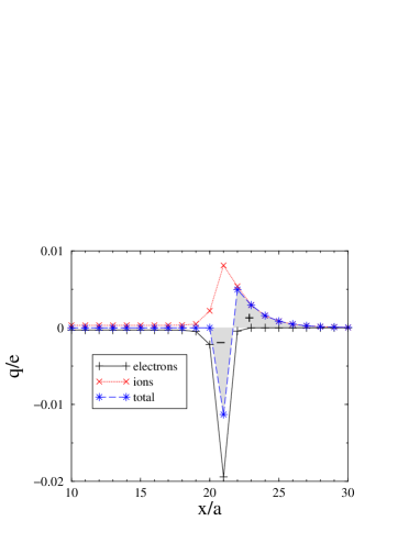
Figure 9: Charge distribution ($q=q^{\alpha}p^{\alpha}$ for species $\alpha$) across the interface of Fig. 8.

In Fig. 9, we show the charge distribution that corresponds to the profile of Fig. 8. Several features are noteworthy. The small homogeneous ion concentrations inside the electrodes are now different for positive and negative ions. This is a direct consequence of the global equilibrium: since the electrochemical potentials are constant throughout the whole system and the ion concentrations in the liquid are fixed, the ion concentrations in the solid are multiplied by factors $\exp(-q^{\alpha}\Delta V/kT)$ with respect to the reference state $\Delta V=0$. The resulting “background charge” in the bulk electrode is exactly compensated by the electrons that have flown in from the metal side of the system. Since the resulting total charge inside the bulk electrode is zero, the potential is constant, which was the original purpose of introducing the electrons. Inside the diffuse interface between electrode and solution, we find a surface charge that is located almost exclusively on one site.

Figure 10: Potential $V$ as a function of $x$ for $\Delta V=0.1kT/e$ and $p_{liq}^{\pm}$=0.0001 (solid line), $p_{liq}^{\pm}$=0.001 (dashed line), and $p_{liq}^{\pm}$=0.01 (dash-dotted line). The thick line segments are exponential fits ($V(x)=\Delta V\exp[-\kappa(x-x_{int})]$) that yield $\kappa=0.0626$, $0.199$, and $0.622$ for the inverse of the Debye length. The predictions of Eq. (33) are $0.0632$, $0.200$, and $0.632$, respectively. The sizes of the simulated cells were $200$, $100$, and $50$ lattice spacings.

In the liquid, we find the diffuse charged layer that is predicted by the classic sharp-interface model of Gouy and Chapman. For an electrolyte that has singly charged ions, $q^{+}=-q^{-}=e$, the potential and the deviations of the concentrations from the bulk liquid values all decay exponentially with the distance from the interface. For example, $V(x)=\Delta V\exp[-\kappa(x-x_{int})]$ with a decay constant

$$\kappa=\sqrt{\frac{2e^{2}p_{liq}^{\pm}}{\epsilon kT}},$$ (33)

the inverse of the Debye screening length, and $x_{int}$ the position of the (sharp) interface. In Fig. 10, we show the potential profile across a cell subjected to a potential difference of $\Delta V=0.1kT/e$ for different ion concentrations. We obtain values for $\kappa$ by an exponential fit of $V(x)$, using $x_{int}$ (the position of the “sharp interface” extrapolated from the far field) as an adjustable parameter. The results are in good agreement with the predictions of Eq. (33). The potential follows an exponential law over several orders of magnitude. However, when the potential approaches its reference value in the liquid, deviations from the exponential behavior occur. This is due to the fact that the buildup of the ion boundary layer at the interface also modifies the chemical potentials for solvent and metal by small amounts. Since the electrochemical potential of the ions depends on the solvent and vacancy concentrations, a complete equilibrium solution must contain these effects. Close to the interface, they are negligible in comparison to the contribution of the electric potential; only far from the interface, when $V-V_{liquid}$ becomes of the same order as the small shifts in the chemical potentials, the deviations from an exponential become appreciable. Since this occurs for fractions of the potential drop that are less than $10^{-3}$ of $\Delta V$, these effects can safely be neglected in the further analysis.

The resulting total charge distribution has the expected double-layer structure, with a much sharper decay in the electrode than in the liquid. We have checked that the integral of the total charge through the interface is zero to numerical precision.

III.3 Electrochemical equilibrium: Nernst law

The electrochemical equilibrium between electrodes and electrolyte depends on the choice of the Fermi energy $E_{F}$. Indeed, consider a chemical equilibrium in the absence of an electric potential such as the one shown in Fig. 6. In this state, the electrochemical potential of the ions is constant across the cell. If we fix $E_{F}$ to be exactly equal to the difference of the chemical potentials of metal and cations,

$$E_{F}^{0}=\mu^{0}_{eq}-\mu^{+}_{eq},$$ (34)

the reaction currents $\sigma$ are strictly zero everywhere as long as the potential remains constant. Therefore, the original profile remains an equilibrium state for arbitrary transfer frequency $w^{\star}$. In contrast, if $E_{F}$ is set to a value different from $E_{F}^{0}$, the electron transfer starts and drives the system to a new equilibrium that exhibits a potential difference.

The final potential difference will be close to $E_{F}-E_{F}^{0}$. This can be deduced as follows. For fixed concentrations and electric potential in the liquid, the electrochemical potentials of the ions and the metal are fixed. Therefore, the only way to achieve equilibrium is to adjust the electric potential in the electrode such that the two terms in Eq. (23) balance. Now consider the electrochemical potential of the electrons. The excess electronic charge $p^{e}$ is always small, $|p^{e}|\ll e\Delta V/kT$, even at the surface, as can be seen in Fig. 9. Since, in addition, we have chosen $\mathcal{D}(E_{F})kT\gg 1$, $\widetilde{\mu}^{e}$ is only weakly dependent on the local electron density. Neglecting the last term in Eq. 14, the electron transfer rate becomes zero when $E_{F}-e\Delta V=E_{F}^{0}$.

We have checked this prediction by performing simulations in isolated cells: the concentrations of all species and the potential were kept fixed at the liquid side, and the system was closed at the solid side for particles and electrons, thus enforcing zero electrical current. For $p^{\pm}_{liq}=0.01$, Eq. (34) yields $E_{F}^{0}/kT=4.447514$. For $E_{F}=E_{F}^{0}$, the system remained at constant potential, whereas for $E_{F}\neq E_{F}^{0}$, the predicted potential difference developed up to an error of less than $10^{-5}$. Since all of the charges can be removed from the system by applying an external potential difference that is just the negative of $(E_{F}-E_{F}^{0})/e$, the choice of $E_{F}$ determines the potential of zero charge (PZC) of the electrochemical interface.

Figure 11: Equilibrium potential difference through an isolated cell versus ion concentration in the liquid for fixed $E_{F}=4.447514\,kT$. The solid line corresponds to Eq. (35).

Of course, the value of $E_{F}^{0}$ as defined above depends on the ion concentration in the liquid. Therefore, for fixed $E_{F}$, there is a well-defined ion concentration $p^{\pm}_{ref}$ for which the potential difference is zero. When the concentration in the liquid is varied, the potential difference follows Nernst’s law,

$$\Delta V={\frac{kT}{e}}\ln{\frac{p^{\pm}}{p^{\pm}_{ref}}}.$$ (35)

In Fig. 11, we plot $\Delta V$ vs $p^{\pm}_{liq}$ for $E_{F}^{0}/kT=4.447514$ (corresponding to $p^{\pm}_{ref}=0.01$). The results of our model are in perfect agreement with Eq. (35).

III.4 Growth

To investigate growth and dissolution, we use one-dimensional cells with a metallic electrode at both ends. The system is closed on both sides for all species (ions, metal, solvent) but open for electrons. To drive the interfaces, we apply a fixed potential difference $\Delta V$ across the cell. For $e\Delta V/kT$ ranging from 1 to 10 and a cell of size 100 with two electrodes of thickness 10, the system reaches a steady state within $5\times 10^{6}$ timesteps ($\Delta t=1$). Within $2\times 10^{7}$ timesteps, the interface advances between 3 and 15 sites, depending on the voltage. We measure the ionic current in the center of the cell by time-averaging over the second half of the runs.

Given the rapid variations of ion concentrations and electronic charges through the interface (see for example Fig. 9), one could expect strong lattice pinning effects Cahn60 ; Kessler90 ; Plapp97b . We have checked that quantities such as the electronic surface charge, the total transfer rate (that is, the transfer currents $\sigma_{\mathbf{k,k+a}}$ summed up through the interface) and the ion current indeed do vary as the interface advances through the lattice. However, for the parameters chosen here, the amplitudes of these lattice oscillations never exceeded a few percent.

The choice of the various time constants does not influence the final results for equilibrium states. In contrast, for growth simulations, they have to be fixed in order to achieve the desired physical conditions. In particular, this is true for the various jump rates and the electron transfer frequency. The electric current in the electrolyte is carried by the mobile ions. As mentioned above, the buildup of the ionic boundary layers shifts the chemical potential of metal, solvent, and vacancies as well. Since, in our model, the concentration of metal in the electrolyte is comparable to the ion concentrations, this leads to neutral diffusion currents that are unphysical. To lower their magnitude, the jump frequency for the metal was chosen much smaller than for the ions: $w^{+}=w^{-}=1$, $w^{0}=10^{-3}$.

Figure 12: Ion current in the center of the cell as a function of the electron transfer frequency $w^{\star}$ for fixed voltage $\Delta V=10\,kT/e$.

In Fig. 12, we plot the ionic current in the center of the cell as a function of the transfer frequency $w^{\star}$ at fixed voltage of 10 $kT/e$. For low transfer frequencies, the growth is limited by the reaction kinetics at the interface, and the current strongly depends on the value of $w^{\star}$. For increasing $w^{\star}$, the growth becomes limited by transport in the bulk, and the current is almost independent of $w^{\star}$. We are mostly interested in the latter regime. Therefore, we fix in the following $w^{\star}=10^{-4}$.

Figure 13: Ion current in the center of the cell as a function of the driving voltage for fixed $w^{\star}=10^{-4}$.

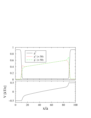
Figure 14: Concentration profiles (top) and potential profile (bottom) across a 100-site cell with initial ion concentration of 0.01 subjected to a potential difference of $\Delta V=kT/e$. The snapshot was taken at $t=2\times 10^{7}$.

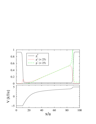
Figure 15: Same as Fig. 14, but for a potential difference of $\Delta V=10\,kT/e$.

The current-voltage curve for our model cell is shown in Fig. 13. It is strongly nonlinear. Indeed, two very different regimes are covered by these simulations. This can be appreciated when looking at the ion and potential profiles in Figs. 14 and 15. For $\Delta V=kT/e$ (Fig. 14), the ion concentrations remain of the same order of magnitude as the initial concentration ($p^{\pm}=0.01$), and except for the two double layers close to the interfaces, the liquid is neutral. An important part of the potential drop occurs in these double layers; in the bulk electrolyte, the potential profile is smooth and almost linear. In contrast, for $\Delta V=10kT/e$ (Fig. 15), the neighborhood of the cathode has been completely depleted of the anions ($p^{-}\sim 10^{-5}$ at the cathode), and a charged zone extends well beyond the thickness of the equilibrium double layers. Most of the potential drop occurs close to the cathode. Since the conductivity in the space-charge zone is lowered due to the low ion concentration, a considerable increase in the overall voltage $\Delta V$ leads only to a moderate increase of the current, as seen in Fig. 13. All of these findings are in good agreement with the macroscopic one-dimensional calculations of Chazalviel Chaza90 . According to this work, the extended space charge is crucial for the emergence of ramified growth: the strong electric field close to the surface leads to an instability of the flat front, and one-dimensional calculations become invalid.

III.5 Two-dimensional simulations: dendritic growth

We present now an example for a preliminary simulation of a two-dimensional sample. The purpose is to show that our model can indeed lead to the emergence of dendritic structures; however, the conditions that we can simulate are far from typical experimental situations. The main reason is that in experiments, the branches of ramified aggregates have typically a thickness in the micron range, whereas the lattice of our model represents a crystal lattice with spacing of the order Ångströms. It is clear that huge simulation cells would be necessary to observe instabilities and ramified growth on realistic scales. To obtain a computationally tractable problem, we have to work with unrealistically high driving forces, since this is known to reduce the characteristic scales of branched growth structures. Therefore, we use a much higher driving potential than in the previous simulations, namely 100 $kT/e$. This corresponds to about 2.5 V at room temperature, which is a fairly typical value; however, this potential difference is applied through a cell that is, as before, 100 lattice sites long, which corresponds to a length of a few nanometers. Therefore, the electric fields are much higher in our simulation than in reality.

Under these conditions, the behavior of the moving interface is quite sensitive to the model parameters, and in particular to the frequency factors for the electron transfer, $w^{\star}$, and the metal jump frequency $w^{0}$ (as before, we take $w^{+}=w^{-}=1$ as a reference value). To assure that the growth is still transport-limited for the higher driving force, $w^{\star}$ has to be chosen large enough; for reaction-limited growth, no morphological instability occurs. The metal jump frequency has to be chosen carefully. On the one hand, if it is too high, bumps on the surface are smoothed out too rapidly by surface diffusion and/or an evaporation-condensation mechanism. On the other hand, if it is too low, the diffusion of metal on the solid side of the interface becomes so slow that the interface profile cannot be maintained, and the metal grows at a concentration far below its equilibrium value mobthesis .

In Fig. 16, we show an example computed with $w^{\star}=6\times 10^{-3}$, $w^{0}=10^{-3}$, and $w^{e}=10^{-3}$. The cell has a size 40 $\times$ 100 lattice sites, with periodic boundary conditions parallel to the interfaces. The simulation was started from a flat interface, with random shifts of the metal concentration in the interfaces to trigger the instability. When one layer of the anode was dissolved, the whole cell was shifted backward by one site in order to keep the electrolyte in the center of the cell. It can be seen that a bump grows on the interface and develops into a finger-like structure. Other bumps that initially develop on the interface are screened. The whole region that surrounds the dendrite is depleted of ions. An extended charged region forms ahead of the tip. When the tip gets closer to the anode, the electric field increases and leads to growth of the metal at unphysically low concentrations.

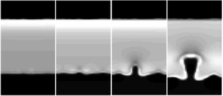
Figure 16: Snapshots of the evolution of a $100\times 40$ electrochemical cell; the parameters are given in the text. The electrodes are in black; the cathode is at the bottom and grows upward (the cell is recentered during the simulation). In the electrolyte, the grayscale indicates the concentration of ions, with white corresponding to the maximal ion concentration. The white “contour” at the electrode surfaces is the charged double layer; the gray region in front of the dendrite has been almost completely depleted of ions.

IV Conclusion

In summary, we have shown here that, starting from a simple microscopic model, it is possible to build Electrochemical-Mean-Field-Kinetic Equations (EMFKE) that are able to reproduce qualitatively the behavior of electrochemical cells. Both the charged double layers present at equilibrium and the extended space charge that develops during growth are correctly reproduced. Dendritic structures can be simulated, albeit for unrealistic parameters. Hence, the EMFKE contain the fundamental ingredients that are necessary to simulate dendritic growth by electrodeposition.

Our model shares many common features with a recent phase-field formulation of electrodeposition GBW . The phase-field method, originally developed in the context of solidification in the 1980s Langer86 ; Collins85 ; Caginalp86 , is a continuous model of phase transitions that uses an auxiliary indicator field, the phase field, to distinguish between the different thermodynamic phases (here, electrodes and electrolyte). A phenomenological equation of motion for the phase field is usually derived from a free energy functional. In our EMFKE approach, the role of the phase field is played by the metal concentration.

Since the phase-field method is phenomenological, it has a certain freedom of choice for the dynamics of the phase field itself, and can hence avoid the problems that arise in our model due to the presence of metal in the electrolyte. However, no direct link to a microscopic model is established, which is the strength of our approach. Our equations still contain some phenomenological elements, in particular, the interpolation function for electron diffusivity and reaction rates. A more realistic modeling of the processes involving electrons is needed to overcome this limitation. With this perspective, our approach may constitute a useful link between microscopic models and phase-field models.

Discussions with J.-N. Chazalviel, V. Fleury, and M. Rosso are greatly acknowledged. Laboratoire de Physique de la Matière Condensée is Unité Mixte 7643 of CNRS and Ecole Polytechnique.

Appendix A The Butler-Volmer equation

On the metal-electrolyte interface, the oxido-reduction reaction,

$$M^{+}(\mathbf{k)}+e^{-}(\mathbf{k+a)}\begin{array}[]{l}k_{red}\\ \rightleftharpoons\\ k_{ox}\end{array}M^{0}(\mathbf{k)}.$$ (36)

is characterized by two rates $k_{ox}$ and $k_{red}$. In our simplified model, the reduction of a cation $M^{+}$ located on a site $\mathbf{k}$ that is nearest neighbor of a surface site, is carried out by the transfer of an electron coming from a site $\mathbf{k+a}$ of the electrode: a reduced metallic atom is then created at site $\mathbf{k}$ on the interface.

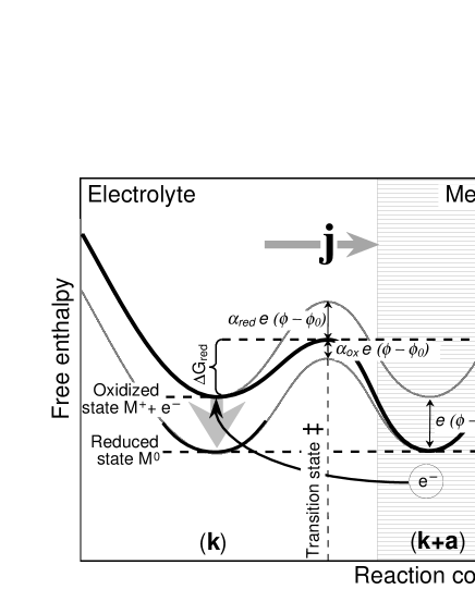
Figure 17: Free enthalpy along the reaction path for the electron transfer. Between the two states $M^{0}$ and $M^{+}+e$, there is a transition state ${\ddagger}$ of higher enthalpy. Therefore, the barriers $\Delta G_{red}$ and $\Delta G_{ox}$ determine the reaction rate. It exists an equilibrium potential $\phi_{0}$ for which $M^{0}$ and $M^{+}+e$ have the same enthalpy, the two barriers are the same, $\Delta G_{red}(\phi_{0})=\Delta G_{ox}(\phi_{0})$, and there is a balance between oxidation and reduction. When a potential $\phi\neq\phi_{0}$ is applied, the relative positions of the states vary, and the barriers are modified. In the figure, the solid line is the free enthalpy at $\phi\neq\phi_{0}$, whereas the two dotted lines are two copies of the equilibrium enthalpy profile, shifted to match the two local minima in the non-equilibrium profile. The definitions of the modified barriers can be read off; since we have $\alpha_{red}e(\phi-\phi_{0})+\alpha_{ox}e(\phi-\phi_{0})=e(\phi-\phi_{0})$, Eq. (39) follows.

The Butler-Volmer model (Fig. 17) supposes that there exists a potential difference $\phi$ between the electrolyte, where the cations $M^{+}$ can be reduced, and the metal of the electrode, where a metallic atom $M^{0}$ can be oxidized. In between, there exists an activation barrier for the redox reaction, and (if we suppose that the frequency prefactors are the same) the corresponding rates are

$$k_{red}=A\exp-\frac{\Delta G_{red}(\phi)}{kT}~{}\quad~{}k_{ox}=A\exp-\frac{\Delta G_{ox}(\phi)}{kT}.$$ (37)

For some potential $\phi_{0}$, the two barriers are equal, $\Delta G_{red}(\phi_{0})=\Delta G_{ox}(\phi_{0})$, and hence $k_{red}=k_{ox}$ such that the total reaction current $\mathbf{j}$ is zero. When $\phi\neq\phi_{0}$ (in the figure $\phi>\phi_{0},$ metal is deposited), the barriers are modified. To first order in $\phi-\phi_{0}$,

$$\Delta G_{red}(\phi) = \Delta G_{red}(\phi_{0})-\alpha_{red}e(\phi-\phi_{0}),$$

$$\Delta G_{ox}(\phi) = \Delta G_{ox}(\phi_{0})+\alpha_{ox}e(\phi-\phi_{0}),$$ (38)

with (see Fig. 17 for an explanation),

$$\alpha_{ox}+\alpha_{red}=1.$$ (39)

The Butler-Volmer relation then gives the electron transfer current

$$\mathbf{j}=\mathbf{j}_{0}\left(\exp\left[\frac{e\alpha_{red}(\phi-\phi_{0})}{kT}\right]-\exp\left[-\frac{e\alpha_{ox}(\phi-\phi_{0})}{kT}\right]\right).$$ (40)

In our present model, we have supposed in Eq. (36) that the reduction of a cation in $\mathbf{k}$ is due to a charge transfer from the metal site $\mathbf{k+a}$. The link with Eq. (23) for the reaction rate can then be established. The electrochemical potentials are

$$\widetilde{\mu}_{\mathbf{k}}^{+}+\widetilde{\mu}_{\mathbf{k+a}}^{e} = \mu_{\mathbf{k}}^{+}+E_{F}-e\Phi_{\mathbf{k+a\rightarrow k}},$$

$$\widetilde{\mu}_{\mathbf{k}}^{0} = \mu_{\mathbf{k}}^{0},$$ (41)

where we have introduced the potential difference

$$\Phi_{\mathbf{k+a\rightarrow k}}=V_{\mathbf{k+a}}-V_{\mathbf{k}}-\frac{p_{\mathbf{k+a}}^{e}}{e\mathcal{D}(E_{F})}.$$ (42)

The equilibrium (absence of reaction) is obtained when $\Phi_{\mathbf{k+a\rightarrow k}}=\Phi_{\mathbf{k+a\rightarrow k}}^{0}$ for which

$$\widetilde{\mu}_{\mathbf{k}}^{+}+\widetilde{\mu}_{\mathbf{k+a}}^{e}=\mu_{\mathbf{k}}^{+}+E_{F}-e\Phi_{\mathbf{k+a\rightarrow k}}^{0}=\mu_{\mathbf{k}}^{0}.$$ (43)

Furthermore, a reaction rate of the form (23) can also be written as

$$\sigma_{\mathbf{k,k+a}} = w_{\mathbf{k,k+a}}^{\star}\left[\exp\left({\alpha_{red}\frac{\widetilde{\mu}_{\mathbf{k}}^{+}+\widetilde{\mu}_{\mathbf{k+a}}^{e}-\widetilde{\mu}_{\mathbf{k}}^{0}}{kT}}\right)\right.$$ (44)

$$\left.\mbox{}-\exp\left({-\alpha_{ox}\frac{\widetilde{\mu}_{\mathbf{k}}^{+}+\widetilde{\mu}_{\mathbf{k+a}}^{e}-\widetilde{\mu}_{\mathbf{k}}^{0}}{kT}}\right)\right],$$

with

$$w_{\mathbf{k,k+a}}^{r}=w_{\mathbf{k,k+a}}^{*}\exp\frac{\alpha_{ox}\left(\widetilde{\mu}_{\mathbf{k}}^{+}+\widetilde{\mu}_{\mathbf{k+a}}^{e}\right)+\alpha_{red}\widetilde{\mu}_{\mathbf{k}}^{0}}{kT}.$$ (45)

With the help of Eq. (41), we obtain

$$\sigma_{\mathbf{k,k+a}} = w_{\mathbf{k,k+a}}^{\star}\left[\exp\left(-{\frac{e\alpha_{red}(\Phi_{\mathbf{k+a\rightarrow k}}-\Phi_{\mathbf{k+a\rightarrow k}}^{0})}{kT}}\right)\right.$$ (46)

$$\quad\left.\mbox{}-\exp\left({\frac{e\alpha_{ox}(\Phi_{\mathbf{k+a\rightarrow k}}-\Phi_{\mathbf{k+a\rightarrow k}}^{0})}{kT}}\right)\right],$$

which has the form of Eq. (40). In the above expressions, for a square or a simple cubic lattice, with intersite distance $a$, the transfer current density is

$$\mathbf{j} = a^{d-1}w_{\mathbf{k,k+a}}^{*}\exp\left[{\frac{\alpha_{ox}\left(\widetilde{\mu}_{\mathbf{k}}^{+}+\widetilde{\mu}_{\mathbf{k+a}}^{e}\right)+\alpha_{red}\widetilde{\mu}_{\mathbf{k}}^{0}}{kT}}\right]$$ (47)

$$\simeq a^{d-1}w_{\mathbf{k,k+a}}^{*}e^{\mu_{\mathbf{k}}^{0}/kT},$$

where the last expression is valid close to equilibrium. In that case, and with the help of Eq. (24) for $w^{*}_{\mathbf{k,k+a}}$, the constant $\mathbf{j}_{0}$ of the Butler-Volmer law can be identified as $\mathbf{j}_{0}=a^{d-1}w^{*}e^{\mu^{0}/kT}$, where $\mu^{0}$ is the equilibrium chemical potential for the metal species. Note that with Eq. (24), our expression is only an approximation to the Butler-Volmer law, valid close to equilibrium; to get a complete correspondence with the Butler-Volmer model, a dependence of $w^{*}$ on the electrochemical potentials needs to be introduced.

References

- (1) C.A. Vincent, B. Scrosati, Modern Batteries, (Edward Arnold Publishers Ltd, London, 1997); see also the web site, http://www.corrosion-doctors.org for general informations on Batteries, corrosion, electrodeposition.
- (2) Biolelectrochemistry: general introduction, edited by S.R Caplan, I.R. Miller, and G. Milazzo (Birkhäuser, Basel, 1995); see also the review “Bioelectrochemistry”, Elsevier Science.
- (3) V. Fleury, Arbres de pierre, la croissance fractale de la matière (Flammarion, Paris, 1998).
- (4) R. Selim and P. Bro, J. Electrochem. Soc. 121, 1457 (1974).
- (5) H. A. Laitinen and I. M. Kolthoff, J. Am. Chem. Soc. 61, 3344 (1939).
- (6) D. P. Barkey, D. Watt, Z. Liu, and S. Raber, J. Electrochem Soc. 141, 1206 (1994).
- (7) J. M. Huth, H. L. Swinney, W. D. McCormick, A. Kuhn, and F. Argoul, Phys. Rev. E 51, 3444 (1995).
- (8) M. Rosso, E. Chassaing, and J.-N. Chazalviel, Phys. Rev. E 59, 3135 (1999).
- (9) M. Rosso, J.-N. Chazalviel, V. Fleury, and E. Chassaing, Electrochim. Acta 39, 507 (1994).
- (10) W. Schmickler, Interfacial Electrochemistry (Oxford University Press, Oxford, 1996).
- (11) M. Matsushita, M. Sano, Y. Hayakawa, H. Honjo, and Y. Sawada, Phys. Rev. Lett. 53, 286 (1984).
- (12) D. Grier, E. Ben-Jacob, R. Clarke, and L.M. Sander, Phys. Rev. Lett. 56, 1264 (1986).
- (13) Y. Sawada, A. Dougherty, and J.P. Gollub, Phys. Rev. Lett. 56, 1260 (1986).
- (14) V. Fleury, M. Rosso, J.-N. Chazalviel, and B. Sapoval, Phys. Rev. A 44, 6693 (1991).
- (15) T. A. Witten and L. M. Sander, Phys. Rev. Lett. 47, 1400 (1981); Phys. Rev. B 27, 5686 (1983).
- (16) T. Vicsek, Phys. Rev. Lett. 53, 2281 (1984).
- (17) J. Nittmann and H. E. Stanley, Nature 321, 663 (1986).
- (18) J.-P. Eckmann, P. Meakin, I. Procaccia, and R. Zeitak, Phys. Rev. A 39, 3185 (1989).
- (19) P. Meakin, Phys. Rev. B 28, 5221 (1983).
- (20) R. Jullien, M. Kolb, and R. Botet, J. Phys. (France) 45, 395 (1984).
- (21) S. C. Hill and J. I. D. Alexander, Phys. Rev. E 56, 4317 (1997).
- (22) G. Marshall and P. Mocskos, Phys. Rev. E 55, 549 (1997).
- (23) J. Elezgaray, C. Léger, and F. Argoul, Phys. Rev. Lett. 84, 3129 (2000).
- (24) P.A. Rikvold, G. Brown, M.A. Novotny, and A. Wieckowski, Colloids and Surfaces A: Physicochemical and Engineering Aspects 134, 3 (1998).
- (25) W. Schmickler, J. Electroanal. Chem. 460, 144 (1999).
- (26) G. Martin, Phys. Rev. B 41, 2279 (1990).
- (27) J.-F. Gouyet, Europhys. Lett. 21 , 335 (1993).
- (28) V. Vaks, and S.Beiden, Sov. Phys. JETP 78, 546 (1994).
- (29) J.-F. Gouyet, Phys. Rev. E 51, 1695 (1995).
- (30) V. Dobretsov, V. Vaks, and G. Martin, Phys. Rev. B 54, 3227 (1996).
- (31) M. Plapp and J.-F. Gouyet, Phys. Rev. Lett. 78, 4970 (1997); Eur. Phys. J. B. 9, 267 (1999).
- (32) M. Plapp and J.-F. Gouyet, Phys. Rev. E 55, 45 (1997).
- (33) M.-O. Bernard, M. Plapp, and J.-F. Gouyet, in Complexity an Fractals in Nature, edited by M. M. Novak (World Scientific, Singapore, 2001), pp. 235-246.
- (34) M.-O. Bernard, M. Plapp, and J.-F. Gouyet, Physica A, in press.
- (35) J. E. Guyer, W. J. Boettinger, J. A. Warren, and G. B. McFadden, in Design and Mathematical Modeling of Electrochemical Systems, edited by J. W. Van Zee, M. E. Orazem, T. Fuller, and C. M. Doyle (Electrochemical Society, Pennington, NJ, 2002).
- (36) J.-N. Chazalviel, Phys. Rev. A 42, 7355 (1990).
- (37) J. W. Cahn, Acta Metall. 8, 554 (1960).
- (38) D. A. Kessler, H. Levine, and W. N. Reynolds, Phys Rev. A 42, 6125 (1990).
- (39) M. Plapp and J.-F. Gouyet, Phys. Rev. E 55, 5321 (1997).
- (40) J.-N. Chazalviel, Coulomb Screening by Mobile Charges (Birkhäuser, Basel, 1999), pp. 22-27.
- (41) For more details on the two-dimensional simulations and the relation between parameters and morphologies, see M.-O. Bernard, Ph. D. Thesis, Ecole Polytechnique (Palaiseau, France, 2001), electronic version available at http://tel.ccsd.cnrs.fr
- (42) J. S. Langer, in Directions in Condensed Matter, edited by G. Grinstein and G. Mazenko (World Scientific, Singapore, 1986), p. 164.
- (43) J. B. Collins and H. Levine, Phys. Rev. B 31, 6119 (1985).
- (44) G. Caginalp and P. Fife, Phys. Rev. B 33, 7792 (1986).