Finite size effects and localization properties of disordered quantum wires with chiral symmetry

Abstract

Finite size effects in the localization properties of disordered quantum wires are analyzed through conductance calculations. Disorder is induced by introducing vacancies at random positions in the wire and thus preserving the chiral symmetry.

For quasi one-dimensional geometries and low concentration of vacancies, an exponential decay of the mean conductance with the wire length is obtained even at the center of the energy band. For wide wires, finite size effects cause the conductance to decay following a non-pure exponential law. We propose an analytical formula for the mean conductance that reproduces accurately the numerical data for both geometries. However, when the concentration of vacancies increases above a critical value, a transition towards the suppression of the conductance occurs. This is a signature of the presence of ultra-localized states trapped in finite regions of the sample.

I Introduction

Disorder effects in the transport properties of quantum wires have been the subject of extensive investigations in recent years. Among these works, models with pure off-diagonal disorder have been studied in connection to peculiar properties that seem to differentiate them from models with pure diagonal disorder only eilmes ; brouwer1 ; brouwer2 ; mudry ; verges . Unusual phenomena like anomalies in the density of states (DOS) and in the localization properties of quantum wires have been reported for a random hopping model of disorder in the vicinity of energy $E=0$. As an example, in Refs. brouwer1 ; brouwer2 ; mudry the authors pointed out that, for a wire with an odd number of channels and at the band center, the conductance decays algebraically with the wire length rather than exponentially, as is usual in the problem of Anderson localization lee . These behaviors have been attributed to the existence of a delocalized state at $E=0$ that arises as a consequence of an additional lattice symmetry, absent in models with pure diagonal disorder. Due to this symmetry, referred as chiral, the eigenvalues appear in pairs $\pm E$ and the spectrum is symmetric with respect to $E=0$ brouwer1 ; brouwer2 ; mudry .

However, for other models of disorder with chiral symmetry the existence of a delocalized state near the center of the band is still a subject of debate miller ; furu . One source of discrepancy is the large localization length obtained near the center of the band, that makes difficult to decide from numerical data whether or not states are localized.

In view of this controversy, we find instructive to study an alternative model of disorder that, like the random hopping model, has chiral symmetry. The localization properties will be inferred from conductance calculations performed in wire like geometries. Disorder is induced introducing a number of vacancies $N_{v}$ at random positions in a regular lattice that defines the wire. Vacancies represent sites with an infinite energy that block the motion of the electrons. Therefore the only way an electron may propagate across the sample is through a path with no vacancies. This model could be thought as a limiting case of the random site percolation problem koslo known as the binary-alloy model kir ; souk .

For quasi-one dimensional wires we show that, unlike the random hopping model, the present model of disorder exhibits exponential localization at the band center irrespective of the parity in the number of transmission channels. We propose an analytical formula that reproduces the behavior of the mean conductance as a function of the vacancy concentration. For wide wires, as finite size effects become important in the mesoscopic regime, a detailed analysis of the influence of the geometry on the conductance and on the localization properties will be performed.

As the vacancy concentration increases above a critical value we show that ultra-localized states are formed. These states influence dramatically the value of the conductance and a transition towards the suppression of the conductance in the wires is observed.

The present model supports the conjecture that the chiral symmetry appears to be a necessary but not a sufficient condition for the existence of anomalies at the band center in the localization properties of disordered quantum wires.

II Conductance calculations

The wires are stripes of length $L$ and width $W$ defined on a square lattice. We employ the tight-binding Hamiltonian with a single atomic level per site :

$$H=-\sum_{i,j_{i}}{\hat{c}_{i}}^{\dagger}{\hat{c}}_{j_{i}}\;,$$ (1)

where the operator $\hat{c_{i}}$ destroys an electron on the site $i$. All the hopping integrals are taken equal to $-1$ and restricted to nearest neighbors. $j_{i}$ labels only the existing nearest-neighbors of site $i$ after introducing $N_{v}=\alpha\;W\;L$ vacancies at random positions. Ideal leads of width $W$ are attached at both ends of the sample through hopping integrals equals to $-1$ and enter in the Hamiltonian Eq.(1) as complex self-energies datta . The Landauer formalism landau is employed to calculate the conductance for each realization of disorder. Open boundary conditions are imposed in the direction transverse to conduction.

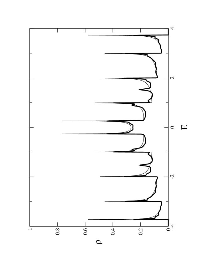
Figure 1: Density of states (DOS) $\rho$ as a function of the energy $E$ for a clean quantum wire (thin line) of $W=5$ and $L=100$ and for the same geometry but when $\alpha=.02$ (thick line). The chirality manifests in the symmetry with respect to the $E=0$ axis.

The present model of disorder has chiral (particle - hole) symmetry. This is illustrated in Fig. 1, where we plot the DOS as a function of the energy $E$ for a wire of $W=5$ and $L=100$. For comparison we show the ideal situation (without vacancies) and when the concentration of vacancies is $\alpha=.02$. In both cases, the chiral symmetry is manifested in the symmetry of the spectrum with respect to the $E=0$ energy axis.

The conductance of a quantum wire of width $W$ which supports $N(E)$ open channels,

$$G\equiv\sum_{n=1}^{N(E)}g^{(n)}\;=\frac{e^{2}}{\hbar}\sum_{n,m=1}^{N(E)}|t_{n,m}|^{2}\;,$$ (2)

is related to the transmission amplitudes $t_{n,m}$ connecting the incoming mode $n$ at the entrance lead with the outgoing mode $m$ in the exit lead. Therefore for a perfect wire with no vacancies it is well known that the dimensionless conductance $g\equiv G/({e^{2}}/{\hbar})$ increases in one unit when a new incoming channel is opened. For $N(E)$ open channels is $g=N(E)$, and at the band center $g(E=0)=N(E=0)=W$.

In the following we will perform conductance calculations as a function of the vacancy concentration $\alpha$. We will focus on the results at the band center ($E=0$). This is the special energy value for which anomalies in the conductance have been reported in the random hopping model of disorder brouwer1 ; brouwer2 ; mudry . We will obtain an analytical formula that reproduces quite satisfactory the behavior of the mean conductance as a function of the vacancy concentration for quasi-one dimensional wires and also for wide wires in which $W\lesssim L$.

II.1 Quasi-one dimensional wires

Here we present conductance calculations for quasi-one dimensional wires where $W<<L$. Averages over configurations of disorder have been performed to obtain the mean conductance, that unless other specification we will denote for simplicity with the symbol $\bf g$. The total number of vacancies for each concentration is $N_{v}=\alpha\;L\;W$.

We start analyzing the effect of $N_{v}=1$ vacancy on the conductance. Due to the fact that the perfect wire has translation symmetry along the longitudinal direction ($\bf x$), the wire with one vacancy has inversion symmetry along this direction with respect to a transverse line that contains the vacancy. Therefore the wave functions of the system with one vacancy can be written as linear combinations of products of plane waves along the direction of conduction and functions with a node in the site of the vacancy in the the transverse direction to conduction (along the $\bf y$ line that contains the site of the vacancy). Then, due to the chiral symmetry, the number of active transverse modes at energy $E=0$ is determined by the number of independent solutions of the isolated vertical line that contains $W-1$ sites. It is exactly $W-1$. Therefore the value of the conductance is reduced in one unit with respect to the value in the clean wire. That is ${\bf g}_{1}=W-1$, where the subscript refers to the number of vacancies and it is understood that $E=0$.

If a second vacancy is added at the same $y$ than the first one but at a different coordinate $x$, the number of transverse modes remains the same as in the case of one vacancy. Therefore the conductance at $E=0$ is still $W-1$. On the other hand, if the second vacancy is put at the same $x$ coordinate than the first one, but at a different $y$ coordinate, the number of transverse channels is reduced by two with respect to the value in the clean case. Therefore the conductance at $E=0$ would be $W-2$. For any other spatial location of the second vacancy, the separability among the transverse and longitudinal modes is lost. This implies that the conductance will not be $\it{exactly}$ an integer number any more. In order to have an insight about how the conductance is modified in a generic situation, we will keep in mind that the effect of a single vacancy in a clean wire is to cut exactly one channel regardless the spatial location of the vacancy in the sample.

Alternatively, we could calculate the (mean)conductance of a wire with only one vacancy as the sum of the individual conductances of $W$ single channel conductors, each one with a mean conductance of $(W-1)/W$. This gives ${g}_{1}=W\left((W-1)/W\right)=W-1$, as we previously obtained. In the following to compute the conductance we imagine the wire as composed of single-channel conductors in parallel. This approximation neglects interference effects among the different transverse channels when vacancies are added and relies in the fact that the wire is quasi-one dimensional (i.e. the energy separation between transverse modes is very large). The effect of the second vacancy will be to suppress exactly one channel in a “ clean wire” composed by W single channel conductors, each one with a mean conductance of $(W-1)/W$. Therefore the conductance for $N_{v}=2$ can be calculated as the sum of the conductances of $W-1$ single channel conductors each one with an average conductance of $(W-1)/W$. This gives ${g}_{2}=(W-1)\;(W-1)/W\;=W\;\left((W-1)/W\right)^{2}$.

Following this simple scheme up to $N_{v}$ vacancies we obtain

$${g}_{N_{v}}=W\;\left(\frac{W-1}{W}\right)^{N_{v}}=\;W\exp\left(-\;\alpha\;W\log\;\left({\frac{W}{W-1}}\right)L\right)\;;$$ (3)

where we have replaced in the right hand side $N_{v}=\alpha\;W\;L$ in order to show explicitly the exponential decay of the mean conductance with the length of the sample.

Therefore, from Eq.(3) one concludes that the quasi-one dimensional wire with $N_{v}$ vacancies could be model as $W$ single channel conductors in parallel, each one with an average conductance of $\left((W-1)/W\right)^{N_{v}}$.

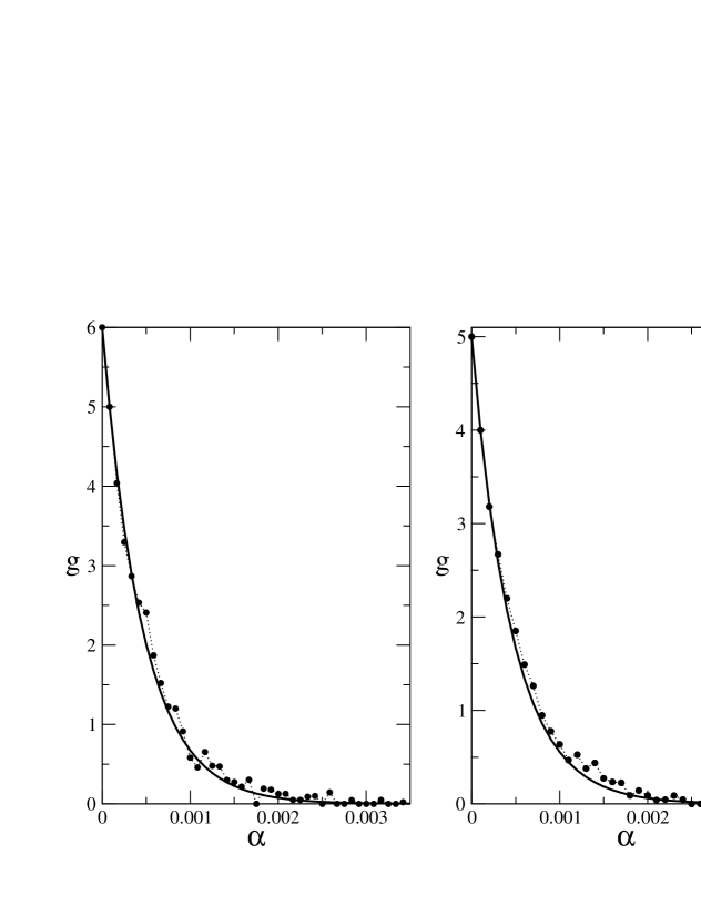
Figure 2: Left panel: Mean conductance $\bf g$ (for $100$ realizations of disorder) at the band center $E=0$, as a function of the vacancy concentration $\alpha$ for a quantum wire of $W=6$ and $L=2000$. The dots are the numerical results and the full line is the analytical estimate given by Eq. (3). Right panel: Idem as left panel but for a wire of $W=5$ and $L=2000$.

In the left (right) panel of Fig. 2 we show $\bf g$ as a function of the vacancy concentration $\alpha$ for a wire of width $W=6\;(W=5)$ and $L=2000$. The solid line in both panels shows the exponential law, Eq.(3), that follows accurately the numerical results (dots) for an ample range of values of $\alpha$. It is interesting to remark that the localization properties of this model do not depend on the parity of the number of transverse channels as it happened in the random hopping model studied in Refs. brouwer1 ; brouwer2 ; mudry .

An analytical estimate of the localization length $\xi$ can be obtained from Eq.(3),

$$\xi=\frac{1}{\alpha\;W\log\left(\frac{W}{W-1}\right)},$$ (4)

which in the limit of $W\sim 1$ gives $\xi\sim 0$. This is consistent with the fact that only one vacancy suffices to suppress the conductance of a one-dimensional wire, that is ${g}_{1}=0$ for $W=1$, as we have previously obtained. Moreover, when $\alpha\sim 1/L$, that is when $N_{v}\sim W$, the conductance becomes lower than one, in agreement with Eq.(3) and the model of W independent channels.

In the limit $1<<W<<L$ is $\xi\sim 1/\alpha$. When $W<<L$, it is satisfied that the mean free path ${\ell}$ and the localization length $\xi$ are related by $\xi=\;W{\ell}$ datta . Thus ${\ell}=L/N_{v}$, as expected for quasi-one dimensional samples.

II.2 Wide wires: finite size effects

When the aspect ratio of the sample $r\equiv W/L$ increases interference effects between the transverse channels become relevant. Therefore the conductance can not be calculated as a sum of the conductances of one-dimensional wires. As a consequence one should expect that Eq. (3) departs from the numerical results when the aspect ratio $r\lesssim 1$.

As was already mentioned, when vacancies are added at arbitrary locations in the sample, the wave functions can not be written as products of functions of the longitudinal coordinate by functions of the transverse coordinate. Disorder mixes the transverse and longitudinal modes and then the separability is lost.

When the first vacancy is added, exactly one channel is suppressed. This is the maximum suppression possible when a site is eliminated and it is due to the fact that the “one vacancy problem” is separable, as was already discussed. However, due to the mixing between channels, when a new vacancy is added that maximum value is not attained and less than one channel is effectively eliminated. Therefore the efficiency of the vacancies for decreasing the conductance is reduced.

In a classical picture the carriers can now propagate following non rectilinear paths along the direction of conduction, avoiding the obstacles (vacancies). Therefore, even after including the rescaling of the mean conductance per channel each time a new vacancy is added (as it was done when we obtained Eq.(3)), the actual conductance for a given value of $\alpha$ should be greater than the value predicted by the pure exponential decay Eq. (3).

Taking into account the effect described above, we propose for wide wires the following ansatz for the mean conductance as a function of $\alpha$,

$${\bf g}=W\;\exp\left(-\;\alpha\;W\;\log{\left({\frac{W-\;\beta}{W-\;1+\beta}}\right)}\;L\right)\;;$$ (5)

with $\beta\equiv(\alpha)^{r}\;(1-\alpha^{r/2})$. For $\alpha<<1$ or $r<<1$, $\beta\to 0$ and the pure exponential decay predicted in Eq.(3) is reobtained.

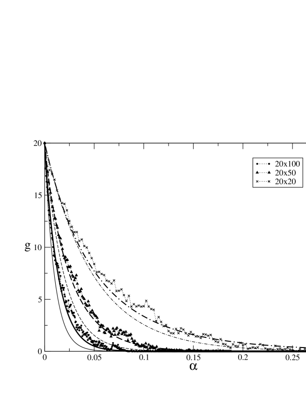
Figure 3: Mean conductance $\bf g$ at $E=0$, as a function of the vacancy concentration $\alpha$ for quantum wires of $W=20$ and $L=100$ (the dots are the numerical results, the full line is the analytical estimate given by Eq. (3) and the thick full line is the analytical estimate given by Eq. (5)), $L=50$ (the triangles are the numerical results, the thin dashed line is the analytical estimate given by Eq. (3) and the thick dashed line is the analytical estimate given by Eq. (5)) and $L=20$ (the crosses are the numerical results, the thin dotted-dashed line is the analytical estimate given by Eq. (3) and the thick dotted-dashed line is the analytical estimate given by Eq. (5)).

In Fig. 3 we show the conductances as a function of $\alpha$ for three different samples with $W=20$ and $L=20,50$ and $100$. The aspect ratios are $r=1,0.4$ and $0.2$ respectively. It is clear that even for relatively small concentrations, the pure exponential formula Eq.(3) departs from the numerical results. On the other hand Eq.(5) gives a quite satisfactory fit to the numerical results even for large concentrations (see the caption in Fig.3).

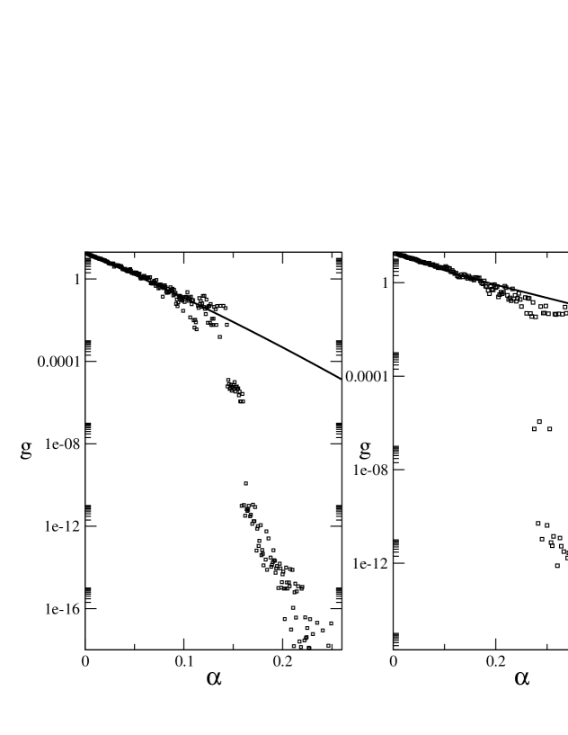
Figure 4: Left panel: Log-Lin plot of the mean conductance $\bf g$ at $E=0$ as a function of $\alpha$ for a quantum wire of $W=20$ and $L=70$ (the squares are the numerical results and the full line is the analytical estimate given by Eq. (5)). Right panel: Idem as left panel but for a wire of $W=20$ and $L=20$.

However, there is a critical value of the concentration above which the conductance falls abruptly towards $0$. Fig.4 shows in a log-lin plot the numerical values for the mean conductance together with those predicted by Eq.(5) for two samples with $W=20$ and $L=70$ and $L=20$ respectively. In both plots, and in spite of the numerical fluctuations, the fall of the conductance towards $0$ is clearly observed. The suppression of the conductance is a signature of the presence of ultra-localized states formed by effect of the vacancies at $E=0$. These ultra-localized states correspond to eigenstates of the disorder isolated $W\dot{L}$ stripe which persist even after the system is embedded with the leads (i.e. these eigenstates extend along a distance $d<L$). To illustrate this point, we evaluate the DOS for a wire (stripe with leads) and two values of the concentration $\alpha$, below and above the critical value ($\alpha_{0}$) respectively. In order to put in evidence the existence of ultra-localized states, we include in the computation of the DOS a small imaginary part $\delta$, such that $\rho(E)\equiv Im\sum_{j}1/(H-\;E+i\;\delta)_{jj}$. The small quantity $\delta$ does not modify the DOS when ultra-localized states are absent (remember that we are computing the DOS for an open system). On the other hand, when the ultra-localized states exist, a single pole in the DOS will appear at $E=0$. It corresponds to a peak with a height that increases linearly with $1/\delta$ as $\delta\rightarrow 0$.

Figure 5 shows the DOS as a function of the energy $E$, $\rho(E)$, for a wire of $L=50$ and $W=20$ and two concentrations $\alpha=0.02<\alpha_{0}$ and $\alpha=0.2>\alpha_{0}$ ($\alpha_{0}\sim 0.12$ for this sample).

The peak in the DOS at $E=0$ for $\alpha=0.2$ is the signature of the presence of ultra-localized states which are trapped in finite regions of the sample defined by the spatial distribution of the vacancies. It should be remarked that it is not necessary that the vacancies enclose completely the region in which the state is trapped, as it was already noted in Ref. kir .

It is worth to mention that the smooth part of the DOS (that is obtained with $\delta=0$) at $E=0$ has a dip but it is not zero, showing the coexistence of ultra-localized states and generic states at the same energy. As the conductance falls down to zero for concentrations $\alpha>\alpha_{0}$, they should be spatially disconnected (indeed the extended states must necessary come from the leads). Therefore when ultra-localized states are formed, the transport across the wire is forbidden.

As the aspect ratio of a sample increases, the value of $\alpha_{0}$ around which the transition takes place also increases. This is consistent with the fact that interference effects between longitudinal and transverse channels (which are maximized for the square geometries) favors the conduction along the sample.

For $\alpha<\alpha_{0}$, that is before the transition towards the suppression of the conductance occurs, the non-pure exponential law Eq.(5) implies that, unlike the quasi one-dimensional wires, it is not possible to define a localization length in the usual way (i.e. as the inverse of the decay rate in the exponential law for the conductance as a function of the length $L$).

III Conclusions

In this work we study the localization properties of disorder quantum wires. Disorder is simulated distributing vacancies at random positions in the sample and thus preserving the chiral symmetry. Conductance calculations at $E=0$ have been performed as a function of the concentration of vacancies $\alpha$, in quasi-one dimensional and in wide wires, respectively.

For quasi-one dimensional wires we have shown that the conductance decays with the length of the wire following an exponential law irrespective of the parity in the number of transverse channels. This is at odd with previous results reported for the random hopping model of disorder in which the scaling of the conductance at the band center would depend on the parity of the number of transverse channels mudry .

We have derived an analytical formula Eq.(3) that reproduces quite accurately the behavior of the mean conductance for an ample range of concentrations $\alpha$.

For wide wires and low values of $\alpha$ a pure exponential decay of the mean conductance with the length $L$ has been also observed. This exponential localization is consistent with the quantum percolation transition predicted for the binary-alloy model in 2d lattices at $\alpha=0$ souk (all the states are exponentially localized for any amount of disorder in a 2d lattice). Therefore, in an infinite system, only one vacancy is enough to suppress the conductance.

However for wide wires and greater values of $\alpha$, we found that the conductance decays following a non pure exponential law. We have proposed an ansatz, Eq.(5), that takes into account how interference effects between channels affect the conductance of the sample as the concentration $\alpha$ increases. If from Eq.(5) we define

$$\bar{\xi}\equiv\frac{1}{\alpha\;W\log\left(\frac{W-\beta}{W-1+\beta}\right)},$$ (6)

this quantity could be interpreted as a localization length that depends on the finite dimensions of the wire.

Finally, a new abrupt transition to the suppression of the conductance is observed when the concentration of vacancies $\alpha$ goes beyond some critical value $\alpha_{0}$ (which is indeed sample dependent) in a finite system. This transition, which is a signature of the formation at $E=0$ of ultra-localized states trapped in finite regions of the sample, can be also interpreted as the quantum analog of the classical cluster percolation transition (CPT). Classically, the CPT and the suppression of the conductivity occurs at the same critical concentration stau . In a quantum system they could be separated due to the fact that ultra-localized states could be formed in an infinite cluster for a finite value $\alpha_{0}>0$.

The ultra-localized states are poles at $E=0$ of the DOS, even after the leads are included, and therefore should be spatially separated from any other extended state of the leads. We should mention that ultra-localized states at $E=0$ have been already reported for the binary alloy model in isolated samples by Kirkpatrick and Eggarter kir . In addition, we do not observe in the DOS a signature of the presence of ultra-localized states out of the band center when the leads are included.

In an infinite 2d quantum system the conductance is suppressed as soon as a single vacancy is introduced, so the conductance is not a relevant magnitude to detect the quantum CPT. However, as in a finite quantum system there is not a complete suppression of the conductance for finite values of $\alpha$, the conductance can be employed to estimate the critical concentration for the quantum CPT. We are currently working along this line.

Figure 5: DOS $\rho(E)$ for a wire of $W=20$ and $L=50$. The solid (dashed) line corresponds to a concentration $\alpha=0.02\;(0.2)$ below (above) the critical concentration $\alpha_{0}$. The peak at $E=0$ for $\alpha=0.2$, $\rho(0)$, is a signature of the presence of localized states. In order to show that the peak represents a Dirac’s delta function, the inset shows that $\rho(0)$ increases linearly with $1/\delta$ for $\alpha=0.2$ whereas for $\alpha=0.02$ it does not depend on $\delta$ ($\delta$ is the small imaginary part defined to compute $\rho(E)$).

- (1) A. Eilmes, R.A. Röemer and M. Schreiber, Eur. Phys. J. B 1, 29 (1998).
- (2) P. W. Brouwer, C. Mudry and A. Furusaki, Phys. Rev. B 57, 10 526 (1998).
- (3) P. W. Brouwer, C. Mudry and A. Furusaki, Phys. Rev. Lett. 84, 2913 (2000).
- (4) C. Mudry, P. W. Brouwer and A. Furusaki, Phys. Rev. B 62, 8249 (2000).
- (5) J. A. Vergés, Phys. Rev. B 65, 054201 (2002).
- (6) For a review see P.A. Lee and T.V. Ramakrishnan, Rev. Mod. Phys.57, 287 (1985).
- (7) J. Miller and J. Wang, Phys. Rev. Lett. 76, 1461 (1996).
- (8) A. Furusaki Phys. Rev. Lett. 82, 604 (1999) and references therein.
- (9) Th. Koslowski and W. von Niessen, Phys. Rev. B 42, 10 342 (1990) and references therein.
- (10) S. Kirkpatrick and T. P. Eggarter, Phys. Rev. B 6, 3598 (1972).
- (11) C. M. Soukoulis and G. S. Grest, Phys. Rev. B 44, 4685 (1991).
- (12) S. Datta,Electronic Transport in Mesoscopic Systems, Cambridge University Press (1995).
- (13) R. Landauer, IBM J. Res. Dev. 32, 306 (1992).
- (14) For a review on classical percolation and for values of the critical exponents, see for example, D. Stauffer and A. Aharony, Introduction to Percolation Theory, Taylor Francis, London (1992).