“Cosmological” quasiparticle production in harmonically trapped superfluid gases

Abstract

We show that a variety of cosmologically motivated effective quasiparticle space-times can be produced in harmonically trapped superfluid Bose and Fermi gases. We study the analogue of cosmological particle production in these effective space-times, induced by trapping potentials and coupling constants possessing an arbitrary time dependence. The WKB probabilities for phonon creation from the superfluid vacuum are calculated, and an experimental procedure to detect quasiparticle production by measuring density-density correlation functions is proposed.

I Introduction

In a gravitational field with explicit time dependence in the metric, particles and antiparticles can be simultaneously created by quantum fluctuations from the vacuum. By the uncertainty principle, the time scale of the system’s evolution dictates the typical energy of the particles produced BirrellDavies . The process of cosmological particle production, whose condensed matter analogue we shall consider here, is potentially relevant in the expanding early universe, in which phonons experience an acoustic geometry; as a consequence, the expansion of the universe could generate density waves growing into galaxies Sachs .

Attention has of late focused on condensed matter analogs of the curved space-times familiar from gravity, primarily due to their conceptual simplicity and realizability in the laboratory GrishaPhysicsReports ; Artifical ; Wisdom ; BoseCondensate ; CSM ; Leonhardt ; PG ; Schutzhold . Condensed matter systems lend themselves for an exploration of kinematical properties of curved space-times and, in particular, provide a testbed to study the effects of a well-defined and controlled “trans-Planckian” physics, i.e. atomic many-body physics on a microscopic scale, on low-energy quantum effects like Hawking radiation hawking and cosmological particle production. In the present paper, we investigate quantum fields propagating on effective curved space-times backgrounds, for the case of harmonically trapped, dilute superfluid gases with possibly time varying particle interactions. For a perfect, irrotational liquid, described by Euler and continuity equations, it was recognized by Unruh unruh that the action of fluctuations of the velocity potential $\Phi$, around a spatially inhomogeneous and time dependent background, can be identified with the action of a minimally coupled scalar field according to

$$S = \int dtd^{3}x\frac{1}{2\kappa}\left[-\left(\frac{\partial}{\partial t}{\Phi}-{\bm{v}}\cdot\nabla\Phi\right)^{2}+c^{2}(\nabla\Phi)^{2}\right]$$ (1)

$$\equiv \frac{1}{2}\int dtd^{3}x\sqrt{-{\textsf{g}}}{\textsf{g}}^{\mu\nu}\partial_{\mu}\Phi\partial_{\nu}\Phi\,.$$

Here, $\bm{v}$ is the background velocity, $1/\kappa$ the compressibility, and $c$ the speed of sound of the liquid. We use the summation convention over equal indices, unless indicated otherwise. The quantities ${\textsf{g}}^{\mu\nu}$ are the contravariant components of the effective metric tensor related to its covariant components by $\textsf{g}^{\beta\nu}\textsf{g}_{\nu\alpha}=\delta^{\beta}{}_{\alpha}$, and ${\textsf{g}}\equiv{\rm det}\,{\textsf{g}}_{\mu\nu}$ is the determinant of the metric tensor. The action (1) leads to the “relativistic” scalar wave equation

$$\square\,\Phi\equiv\frac{1}{\sqrt{-\textsf{g}}}\partial_{\mu}\left(\sqrt{-\textsf{g}}\;\textsf{g}^{\mu\nu}\;\partial_{\nu}\Phi\right)=0.$$ (2)

In general, the effects of quantum fluctuations described by the quantum version of Eq. (1) are very small and can hardly be observed because of finite temperature and dissipation effects. Therefore atomic superfluids, where both extremely small temperatures and dissipationless flows are possible, attract growing interest for an emerging research field of “experimental cosmology.”

In the following, we study how various curved space-times can be implemented in harmonically trapped superfluid Bose and Fermi gases. As a concrete example, we show how de Sitter and Friedmann-Robertson-Walker (FRW) universes can be “re-created” in superfluid gases. We analyze the quasiparticle production probabilities, leading to a thermal spectrum in the WKB approximation, and discuss an experimental procedure to observe and characterize the excitations produced.

II Quasiparticle metric tensors in harmonically trapped superfluids

II.1 Superfluid action

The hydrodynamic, i.e. long-wavelength action of a trapped superfluid is generally given by

$$S=\int dtd^{3}x\left[\rho\frac{\partial}{\partial t}{\phi}+\frac{\rho}{2}{(\nabla\phi)^{2}}+\epsilon(\rho)+V_{\textrm{trap}}\rho\right],$$ (3)

where the external harmonic potential $V_{\textrm{trap}}({\bm{x}},t)=\frac{1}{2}(\omega_{x}^{2}(t)x^{2}+\omega_{y}^{2}(t)y^{2}+\omega_{z}^{2}(t)z^{2})$ is characterized by the three frequencies $\omega_{i}$, $i=x,y,z$. The trapping frequencies are assumed to be time dependent in an arbitrary manner (we can also conceive of making $\omega_{i}^{2}(t)$ effectively negative by “turning over” the potential, see section III). In the above action, the quantity $\rho$ plays the role of a response or stiffness coefficient to gradients of $\phi$, and equals the total fluid density at absolute zero; the equation of state of the superfluid is given by the energy density functional $\epsilon=\epsilon(\rho)$. (Note that we leave out an overall minus sign in the definition of the action $S$.) We generally set $\hbar=m=1$. The action entails the existence of a velocity potential $\phi$, such that the vorticity is zero except on singular lines, and ensures the validity of Euler and continuity equations for the superfluid velocity ${\bm{v}}=\nabla\phi$. The identification of $\phi$ with the phase of a complex “order parameter” (i.e., the direction of a unit vector in the plane of some abstract space) leads to the quantization of circulation, because $\phi$ is then defined only modulo multiples of $2\pi$. Finally, the above action implies the conjugateness of phase and density quantum variables anderson :

$$[\rho({\bm{x}}),\phi({\bm{x}}^{\prime})]=i\delta({\bm{x}}-{\bm{x}}^{\prime})\,.$$ (4)

These properties, taken together, constitute the canonical definition of a superfluid at $T=0$ khalatni ; leggettBEC . Therefore, Eq. (3) represents the universal action of a simple scalar superfluid at absolute zero made up of elementary bosonic or fermionic atoms, independent of a particular microscopic model.

The simplest example for the equation of state is that of a weakly interacting Bose gas, with $\epsilon_{\textrm{B}}=\frac{1}{2}g\rho^{2}$, where $g$ is the coupling constant, $g=4\pi a_{s}$, with $a_{s}$ the $s$-wave scattering length, characterizing pair collisions of atoms. The scattering length can be tuned using external magnetic fields Feshbach . Another example is a two-component Fermi gas with attractive interactions between atoms of different hyperfine species OHara . The ground state of such a gas is superfluid (in the simplest version, it is the BCS state of a scalar superfluid with $s$-wave pairing), and since the interactions are weak, the BCS gap is small and the equation of state (to exponential accuracy) coincides with that of a free Fermi gas: $\epsilon_{\textrm{F}}=\left[{(3\pi^{2})^{2/3}}/{10}\right]\rho^{5/3}$. To consider all possible cases which have a power law density-dependence of the equation of state, in a generic way, we write

$$\epsilon(\rho)=Ag^{\beta}\rho^{\gamma},$$ (5)

where $A$ is a numerical constant. That is, $\beta=1,\gamma=2$ for a dilute Bose gas, and $\beta=0,\gamma=5/3$ for noninteracting two-component fermions.

In our present context, an important quantity characterizing a superfluid is the so-called “Planckian” energy scale, $E_{\rm Pl},$ i.e. the frequency beyond which the spectrum of the excitations above the superfluid ground state ceases to be phononic and (pseudo-)Lorentz invariance is broken. For a weakly interacting Bose gas $E_{\rm Pl}\sim g\rho$, of order the mean interparticle interaction. In a BCS superfluid, $E_{\rm Pl}$ is determined by the BCS gap: $E_{\rm Pl}\sim\rho^{2/3}\exp[-1/(|g|\rho^{1/3})]$. The complete analogy with a quantum field theory on a fixed curved space-time background given by (1) only exists if all timescales $t_{0}$, describing the evolution of the superfluid, are much larger than the “Planck time”: $t_{0}\gg 1/E_{\rm Pl}$.

II.2 Scaling transformation for Bose and Fermi superfluids

Our approach in the following is based on the so-called scaling transformation Scaling ; PitaRosch ; ScalingG(t) ; Menotti to describe the expansion and contraction of the gas under time dependent variations of the trapping frequencies. It is by now a well-established fact that the hydrodynamic solution for density and velocity of motion for such a system may be obtained from a given initial solution by a scaling procedure both in the bosonic Scaling ; PitaRosch ; ScalingG(t) as well as in the fermionic case Menotti . Defining the scaled coordinate vector ${{\bm{x}}_{b}}={\bm{e}}_{i}x_{i}/b_{i}$, density and velocity are given by the scaling transformations Scaling :

$$\rho({\bm{x}},t) \Rightarrow \frac{\tilde{\rho}({\bm{x}}_{b})}{\mathcal{V}}$$ (6)

$$\phi({\bm{x}},t) \Rightarrow \frac{\dot{b}_{i}}{2b_{i}}x_{i}^{2}+\tilde{\phi}({\bm{x}}_{b},t)\,.$$ (7)

The (dimensionless) scaling volume ${\mathcal{V}}=\prod_{i}b_{i}$ in the density (6) is dictated by particle conservation.

Introducing a new “scaling time” variable by

$$\frac{d\tau_{s}}{dt}=\frac{(g/g(0))^{\beta}}{{\mathcal{V}}^{\gamma-1}},$$ (8)

we rewrite the action (3) in the form

$$S = \int d\tau_{s}d^{3}x_{b}\left[\tilde{\rho}\frac{\partial}{\partial\tau_{s}}\tilde{\phi}+\frac{\tilde{\rho}}{2}F_{i}(\tau_{s}){(\nabla_{bi}\tilde{\phi})^{2}}\right.$$ (9)

$$\hskip 50.00008pt\left.+\tilde{\epsilon}(\tilde{\rho})+V_{\textrm{trap}}({\bm{x}}_{b},0)\tilde{\rho}\right],$$

where the $\tau_{s}$ dependent scaling factors are

$$F_{i}(\tau_{s})=\frac{{\mathcal{V}}^{\gamma-1}}{b_{i}^{2}(g/g(0))^{\beta}}=\frac{1}{b_{i}^{2}}\frac{dt}{d\tau_{s}},$$ (10)

and $\tilde{\epsilon}(\tilde{\rho})=\epsilon(\tilde{\rho})_{|g=g(0)}$; $\nabla_{bi}\equiv\partial/\partial x_{bi}$. The rescaled density $\tilde{\rho}$ has no explicit $\tau_{s}$ dependence (whereas it has explicit dependence on the lab time $t$), and coincides with the equilibrium condensate density profile in the scaling coordinate ${\bm{x}}_{b}$. Where any confusion might arise, we will generally designate scaling variables with a tilde to clearly distinguish them from lab frame variables.

For the relation (10) between the scaling factors and ${b_{i}},g$ to hold true, we must impose the following equations of motion for the scaling parameters $b_{i}$:

$$\ddot{b}_{i}+\omega_{i}^{2}(t)b_{i}=\frac{(g/g(0))^{\beta}\omega_{0}^{2}}{{\mathcal{V}}^{\gamma-1}b_{i}}.$$ (11)

They need to be solved with the initial conditions $b_{i}=1$ and $\dot{b}_{i}=0$. Note that here no summation convention is used in the second term on the LHS. For a sufficiently large cloud, the stationary background solution can be found from the Thomas-Fermi density profile. It is given by using that $\mu=-d\tilde{\phi}/d\tau_{s}$ equals the initial chemical potential, and

$$\frac{d\tilde{\epsilon}}{d\tilde{\rho}}=\mu-V_{\rm trap}({\bm{x}}_{b},0)\,.$$ (12)

The part of the action quadratic in the fluctuations is obtained to be

$$S^{(2)} = \int d\tau_{s}d^{3}x_{b}\left[\delta\tilde{\rho}\frac{\partial}{\partial\tau_{s}}\delta\tilde{\phi}+\frac{\tilde{\rho}}{2}F_{i}{(\nabla_{bi}\delta\tilde{\phi})^{2}}+\frac{1}{2}\tilde{\kappa}\delta\tilde{\rho}^{2}\right],$$

where $\delta\tilde{\rho}=\tilde{\rho}-\tilde{\rho}_{0}$ and $\delta\tilde{\phi}=\tilde{\phi}+\mu\tau_{s}$. The rescaled bulk compressional modulus (inverse compressibility) $\tilde{\kappa}={d^{2}\tilde{\epsilon}}/{d^{2}\tilde{\rho}}$ does not depend on the time $\tau_{s}$, and is identical to $g(0)$ in the bosonic case. After integrating out the density fluctuations, we obtain the effective action for the rescaled phase variable

$$\bar{S}^{(2)}=\int d\tau_{s}d^{3}{x_{b}}\frac{1}{2\tilde{\kappa}}\left[-\left(\frac{\partial}{\partial\tau_{s}}\delta\tilde{\phi}\right)^{2}+\tilde{c}^{2}F_{i}(\nabla_{bi}\delta\tilde{\phi})^{2}\right],$$ (14)

where the squared scaling speed of sound ${\tilde{c}}^{2}=\tilde{\kappa}\tilde{\rho}({\bm{x}}_{b})$. Using the identification with a minimally coupled scalar field, analogous to the one performed in the second line of Eq. (1), the line element in the scaling variables reads

$$ds^{2}=\frac{\tilde{c}}{\tilde{\kappa}}\sqrt{F_{x}F_{y}F_{z}}\left[-{\tilde{c}}^{2}d\tau_{s}^{2}+F_{i}^{-1}dx_{bi}^{2}\right].$$ (15)

The line element takes a particularly simple form for an isotropic superfluid Fermi gas, where $\gamma=5/3$ and thus all $F_{i}=1$, leading to $d\tau_{s}/dt=b^{-2}$. We note that even for this simple case, the metric defined by (15) is not trivial, since $\tau_{s}$ and $t$ are different, and both $\tilde{c}$ and $\tilde{\kappa}$ depend on the radial scaling coordinate ${r}_{b}$. We will see below that in the case that $F_{i}=1$ the scaling transformation is exact, and that therefore no quasiparticle creation occurs in the scaling variable basis, i.e. there is no mixing of negative and positive frequency parts in the time $\tau_{s}$ (quasiparticle creation can take place in the lab frame with time $t$, though, and a lab detector will still see that quasiparticles are “created”).

Identifying $\delta\tilde{\phi}$ with $\Phi$, and going back from scaling coordinates to laboratory frame variables, we recover the action (1), with ${\bm{v}}=(\dot{b}_{i}/b_{i})r_{i}{\bm{e}}_{i}$, and the line element, which is of Painlevé-Gullstrand type, reads PGoriginal ; Matt

$$ds^{2}=\frac{c}{\kappa}\left[-(c^{2}-{\bm{v}}^{2})dt^{2}-2v_{i}dx_{i}dt+dx_{i}^{2}\right],$$ (16)

where $c^{2}=\kappa\rho$ is the squared instantaneous speed of sound. We now assume that space is spherically symmetric, i.e. that $\bm{v}$ has a radial component $v_{r}$ only, that $v_{r}/c=f(r)$ holds, and furthermore $c=c(t)$ is a function of time only. We first apply the transformation $c_{0}d\tilde{t}=c(t)dt$, where $c_{0}$ is some constant (initial) sound speed, connecting the laboratory time $t$ to the time variable $\tilde{t}$. This results in the line element $ds^{2}=(c/\kappa)[-c_{0}^{2}(1-f^{2})d\tilde{t}^{2}-2fc_{0}dtdz+dr^{2}+r^{2}d\Omega^{2}$. We then employ a second transformation $c_{0}d\tau=c_{0}{d\tilde{t}}+fdr/(1-f^{2})$ note , to bring the metric into the form

$$ds^{2}=\frac{c}{\kappa}\left[-\left(1-f^{2}(r)\right)c_{0}^{2}d{\tau}^{2}+\frac{1}{1-f^{2}(r)}dr^{2}+r^{2}d\Omega^{2}\right],$$ (17)

The metric in the above form facilitates comparison with metric tensors in spherically symmetric space-times written in their standard form. E.g., if $f^{2}(r)=2M/r$ is chosen, this line element is conformally equivalent to the Schwarzschild metric, the asymptotically flat vacuum solution of the Einstein equations around a spherically symmetric body with total mass $M$ Weinberg .

III Creating De Sitter and Friedmann-Robertson-Walker universes

The equation of state for Bose superfluids contains the interatomic interaction. Therefore, by varying this interaction, possibly together with the trapping frequencies, expanding clouds of Bose atoms allow for the simulation of a large set of cosmological space-times. We begin by discussing the so-called de Sitter universe, which is a solution of the vacuum Einstein equations characterized by the line element deSitter ; Weinberg

$$ds^{2}=-c^{2}\left(1-\frac{\Lambda}{3}r^{2}\right)d{\tau}^{2}+\left({1-\frac{\Lambda}{3}r^{2}}\right)^{-1}dr^{2}+r^{2}d\Omega^{2}\,,$$ (18)

with $\Lambda$ being the cosmological constant $\equiv$ energy density of the vacuum. Up to the conformal factor $c/g$, the metric (17) coincides with the de Sitter metric (18), provided we require that $v_{r}^{2}/c^{2}=\Lambda r^{2}/3$ and that the speed of sound is a constant in space and time. The speed of sound in the center of the cloud is time independent if:

$$c^{2}={\tilde{c}}^{2}={\textrm{const.}}\quad\Longleftrightarrow\quad g(t)/g(0)=b^{3}(t)\,.$$ (19)

Close to the center of the condensate, $c$ is, in addition, practically spatially independent. Using Eq. (7), we find that $\Lambda={\rm const}.$ provided $b\propto\exp[\lambda t]$, with $\lambda=c\sqrt{\Lambda/3}$. This exponential expansion of the cloud can (asymptotically) be achieved if we turn over the potential, making it expel the particles rather than trapping them: $\omega^{2}(t\rightarrow\infty)=-\lambda^{2}$. The de Sitter horizon, where $v_{r}=c$, is stationary and situated at $r_{h}=c(0)/\lambda$, which is well inside the expanding cloud provided $\lambda\gg\omega_{0}$, where $\omega_{0}$ is the initial trap frequency.

The experimental sequence leading to “condensate inflation” is schematically depicted in Fig.1. We assume that the experiment can be done with one trapped (low-field seeking) and one untrapped (high-field seeking) hyperfine component of the same atomic species. We start from a sufficiently large Bose-Einstein-condensed cloud at small (effectively zero) temperature with all atoms being in the trapped state. Then, we transfer all the atoms to the untrapped state, by flipping the sign of the trapping potential. At the same time, we ramp up the interaction strength, according to condition (19), using a suitable Feshbach resonance Feshbach . As a result of the simultaneous action of the inverted parabolic potential and the increasing interaction energy, the gas cloud experiences a rapid exponential expansion, representing the analogue of cosmological inflation.

In fact, Eq. (19) defines a broad class of Bose superfluid effective space-times. In the present case of isotropic expansion with $b_{i}=b$, we have $t=\tau_{s}$ and, in scaling variables, we obtain up to a conformal factor a Friedmann-Robertson-Walker metric:

$$ds^{2}=\frac{c}{\kappa b^{3}}\left[-c^{2}dt^{2}+b^{2}d{r_{b}}^{2}+b^{2}{r_{b}}^{2}d\Omega^{2}\right].$$ (20)

According to the above form of the metric, the quantity $b$ plays the role of the scaling parameter not only in our condensed matter context, but can be interpreted equally well as the scale factor in the expansion of the universe, with $H\equiv\dot{b}/b$ the Hubble parameter. As demonstrated above, exponential growth of $b$, with constant $H$, corresponds to exponential inflation inflation . The present setup also allows for the simulation of power law inflation inflation ; EMomtensor , with $b(t)\propto t^{\delta}$. The “Hubble parameter” $H$ changes for all exponents $\gamma$ inversely proportional to time $t$, $H\propto 1/t$, and the exponent $\delta=1/2$ corresponds to a “radiation dominated” universe, while the exponent $\delta=2/3$ corresponds to a “matter dominated” universe. An isotropically trapped expanding superfluid gas thus models an isotropic expanding universe. Generically, we can model anisotropic universes with (15), with scaling factors which are different in different spatial directions.

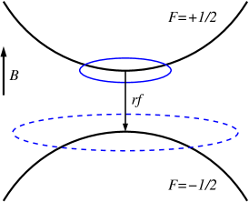
Figure 1: Exponential expansion of a two-component Bose-Einstein condensate with effective spin $F=1/2$, to create a de Sitter quasiparticle universe close to its center. The trapping potential is inverted by applying a radio frequency ($r\!f$) pulse, which transfers the atoms to their untrapped hyperfine state.

While this experiment is feasible in principle, increasing the interaction dramatically increases three-body losses as well, whose total rate scales like $g^{4}\rho^{2}$. This complication can be avoided, by switching to effectively lower-dimensional systems; e.g., a 1+1D analogue of a de Sitter universe can be achieved for quasi-1D excitations in a linearly expanding elongated Bose-condensate, without changing the interaction fedichev:hawkingPRL . Another possibility is to use superfluid Fermi gases. We have, in the isotropic case, $F=1$, $d\tau_{s}=dt/b^{2}$, and the metric may be written in the form

$$ds^{2}=\frac{\tilde{c}}{\beta^{2}\tilde{\kappa}}\left[-\tilde{c}^{2}dt^{2}+\beta^{2}d{r_{b}}^{2}+\beta^{2}{r_{b}}^{2}d\Omega^{2}\right],$$ (21)

where we defined a scale factor $\beta\equiv b^{2}$. Performing experiments in superfluid Fermi gases has the advantage that three-body losses are strongly suppressed by Fermi statistics petrov:3bodyrecfermi .

IV Cosmological particle production analogue

Now we turn to describe the evolution of quantum fluctuations, on top of the classical (mean field) hydrodynamic solutions described above. The equation of motion for the phase fluctuations can be obtained after variation of the action (14),

$$\frac{\partial^{2}}{\partial\tau_{s}^{2}}\delta\tilde{\phi}-\tilde{\kappa}\nabla_{bi}\left(\frac{\tilde{c}^{2}}{\tilde{\kappa}}F_{i}(\tau_{s})\nabla_{bi}\delta\tilde{\phi}\right)=0.$$ (22)

Phrased in curved space-time language, the above equation is the minimally coupled massless scalar wave equation for $\delta\tilde{\rho}$, analogous to (2), with the metric (15).

Consider for simplicity the isotropic case,

$$F_{i}\equiv F=\frac{b^{3\gamma-5}}{(g/g(0))^{\beta}}.$$ (23)

The solution for the full quantum field reads

$$\delta\tilde{\phi} = \sum_{n}\sqrt{\frac{\tilde{\kappa}}{2\tilde{V}\epsilon_{n}}}\phi_{n}({\bm{x}}_{b})\left[{\hat{a}}_{n}\chi_{n}+{\hat{a}}_{n}^{\dagger}\chi_{n}^{*}\right]\,,$$ (24)

where $\tilde{V}$ is the the initial Thomas-Fermi volume of the cloud, the operators $\hat{a}_{n}$ ($\hat{a}_{n}^{\dagger}$) annihilate (create) phonon excitations in the initial vacuum state, and the mode functions $\chi_{n}$ satisfy

$$\frac{d^{2}}{d\tau_{s}^{2}}\chi_{n}+F(\tau_{s})\epsilon_{n}^{2}\chi_{n}=0.$$ (25)

The initial conditions $\chi_{n}(\tau_{s}\rightarrow-\infty)=\exp[-i\epsilon_{n}\tau_{s}]$ are selected such that Eq. (24), at $t\rightarrow-\infty$, describes the phase fluctuations in a static trapped superfluid in its ground state. In quantum field theory (QFT) language this ensures that a laboratory frame detector does not detect quasiparticles at $t\rightarrow-\infty$. Hereafter we define the “scaling vacuum” to be the quantum state annihilated by the operators $\hat{a}_{n}$, where our choice of the initial conditions gurantees that the initial superfluid vacuum and the scaling vacuum coincide at $t\rightarrow-\infty$.

The case when all $F_{i}\equiv 1$ is remarkably special: In this case Eq. (25) does not depend on the superfluid evolution, and thus the quantum state of the excitations remains unchanged. As we have seen above, this indeed happens in the case of an isotropic Fermi superfluid. Another example is a 2D isotropic dilute Bose gas with constant particle interaction PitaRosch . In these cases the scaling transformation is exact, both for the condensate and the excitations. In the language of QFT this amounts to the fact that there is no particle production in the scaling basis, since the scaling solution is constructed from eigenfunctions of the (exactly conserved) scaling transformation operator $F_{i}$ (in other words the scaling vacuum is protected by an exact scaling invariance which forbids frequency mixing). The fact that no excitations are produced in the scaling basis does not mean that a lab detector does not detect quasiparticles. The transformation from the laboratory time $t$ to the scaling time $\tau_{s}$ time is nontrivial and thus the phase of the functions $\chi_{n}$ is a complicated function of the laboratory time $t$. In other words, the phase field given by Eq. (24), if coupled to a detector of the type considered in fedichev:hawkingPRL , gives a non-zero response. This indeterminacy of the vacuum state finds its counterpart in the Unruh-Davies effect in flat space-time unruh76 ; BirrellDavies and its curved space-time generalization, the Gibbons-Hawking effect Gibbons .

The description of a quantum field state in terms of particles and antiparticles is based upon the separation of positive and negative frequency parts. As we confine ourselves to a measurement involving the laboratory time variable $t$, this distinction is only possible if the asymptotic phase of $\chi_{n}$-functions is large and sufficiently quickly increases as a function of $t$. Using a WKB approximation to the solutions of Eq. (25), we find

$$\lim_{t\rightarrow\infty}\int^{t}\sqrt{F}\,\frac{d\tau_{s}}{dt}dt\neq 0.$$ (26)

The latter condition can be also called a “Trans-Planckian safety condition” (TP condition), since if fullfilled it implies that an experiment in a lab frame probing an energy scale $E_{0}\ll E_{\rm Pl}$ does not require information about solutions of Eq. (25) with $\epsilon_{n}\gtrsim E_{\rm Pl}$. For isotropic expansion of a 3D Bose gas, Eq. (26) is equivalent to divergence of $\int dtg^{1/2}/b^{5/2}$ and is quite restrictive: For the FRW analogy discussed above avoiding the divergence implies, according to (19), that $b$ should not grow faster than linearly. The TP condition (26) is based upon the WKB approximation condition for Eq. (25), leading to the requirement $F(\tau_{s})\gtrsim(\epsilon_{n}\tau_{s})^{-2}$ for large $\tau_{s}$ (here $\gtrsim$ means “grows faster than”). Substituting the latter condition into Eq. (26) we find that the marginal WKB case corresponds to a logarithmically divergent integral in Eq. (26). Thus the marginal TP case corresponds to the marginal WKB case and vice versa.

The equation (25) is formally equivalent to scattering of a non-relativistic particle with energy $\epsilon_{n}$ by a potential $\epsilon_{n}^{2}(1-F(\tau_{s}))$. The initial conditions correspond to a single particle per unit time incident on the potential barrier. Time dependence of the scaling factors leads to scattering of the particles from the incoming wave and at $\tau_{s}\rightarrow\infty$ the WKB solution reads:

$$\chi_{n}=\frac{1}{F^{{1}/{4}}}\left(\alpha_{n}e^{-i\epsilon_{n}\int{d\tau_{s}}\sqrt{F}}+\beta_{n}e^{i\epsilon_{n}\int{d\tau_{s}}\sqrt{F}}\right),$$ (27)

where $\alpha_{n}$ is the transmission and $\beta_{n}$ the forward scattering amplitude. The coefficients $\alpha_{n}$ and $\beta_{n}$ are related via the particle flux conservation condition:

$$|\alpha_{n}|^{2}-|\beta_{n}|^{2}=1.$$ (28)

In QFT language the latter condition is the Bogoliubov transformation normalization condition for a bosonic field. The number of particles detected by a scaling time detector at rest is measured by the absolute square $|\beta_{n}|^{2}$ (which is proportional to the probability that the detector absorbs a quantum), and therefore $N_{n}=|\beta_{n}|^{2}$ can be interpreted as the number of scaling basis quasiparticles created.

In the WKB approximation the amplitudes are connected in a simple way:

$$\beta_{n}=\exp[-\epsilon_{n}/2T_{0}]\alpha_{n},$$ (29)

where the inverse temperature is given by the integral

$$\frac{1}{T_{0}}={\Im}\left[\int_{\cal C}\sqrt{F}\,d\tau_{s}\right],$$ (30)

and $\cal C$ is the contour in the complex $\tau_{s}$-plane enclosing the closest to the real axis singular point of the function $F(\tau_{s})$ ll . Together with Eq. (28), this gives

$$N_{n}=|\beta_{n}|^{2}=\frac{1}{\exp[\epsilon_{n}/T_{0}]-1},$$ (31)

i.e. adiabatic evolution of trapped gases leads to “cosmological” quasiparticle creation with thermal occupation numbers in the scaling basis. The temperature $T_{0}$ depends on the details of the scaling evolution (see the specific example in Eq. (37) below).

Interestingly, the evolution of the scaling parameters $b_{i}$, and therefore the nontrivial line element (15), can be generated already in a non-expanding cloud with time-dependent interaction $g(t)$. A similar experiment has been suggested in BLVFRW , where time dependent interactions were used to simulate FRW cosmologies and quantum quasiparticle production. The difference to our approach is due to the fact that the authors of BLVFRW consider a trap with very steep walls (effectively a hard-walled container), so that the density of the cloud does not change, and the superfluid velocity vanishes everywhere at all times. In our setup, we are able to induce cosmological quasiparticle production in a harmonically trapped gas, by changing simultaneously the harmonic trapping and the interaction. The simplest case we can consider is to leave all $b_{i}=1$, like in a stationary Bose condensate. We then create “cosmological” quasiparticles just by changing $g$ (using Feshbach resonances, cf., e.g., Refs. Feshbach ), and accordingly change the trap frequencies $\omega_{i}=\omega$ (in the isotropic case). Following Eqs. (8), (10) and (11), we then have the simple relations

$$\frac{\omega^{2}(t)}{\omega_{0}^{2}}=\frac{g(t)}{g(0)}=\frac{d\tau_{s}}{dt}=\frac{1}{F(t)}.$$ (32)

The metric associated with such a thermal quasiparticle universe created by “shaking the trap” and simultaneously changing the interaction appropriately reads, from Eq. (15)

$$ds^{2} = \frac{\tilde{c}\sqrt{F}}{g(0)}\left[-{\tilde{c}}^{2}Fd\tau_{s}^{2}+d{x_{i}}^{2}\right].$$ (33)

Now, defining the scale factor of the BEC quasiparticle universe by the relation

$$a^{2}_{\rm scal}\equiv\frac{\tilde{c}}{g(t)/g(0)},$$ (34)

we have, up to the (irrelevant) factor $1/g(0)$,

$$ds^{2}=-a^{6}_{\rm scal}d\tau_{s}^{2}+a^{2}_{\rm scal}d{x_{i}}^{2}.$$ (35)

This is the form of the metric employed in BLVFRW , where it was used to calculate cosmological quasiparticle production, inspired by a model of Parker Parker . Note that here a nontrivial scale factor is induced without expanding the cloud. We see from relations (32) and (34) that the scale factor $a_{\rm scal}$ is in our harmonically trapped case simply proportional to the ratio of initial and instantaneous trapping frequencies, $a_{\rm scal}=\sqrt{\tilde{c}}\,\omega_{0}/\omega(t)$.

In Ref. BLVFRW , a specific choice of the scale function $a_{\rm scal}(\tau_{s})$ was taken for the calculation of the quasiparticle creation process,

$$a_{\rm scal}^{4}(\tau_{s})=\frac{a_{\rm scal,i}^{4}+a_{\rm scal,f}^{4}}{2}+\frac{a_{\rm scal,f}^{4}-a_{\rm scal,i}^{4}}{2}\tanh\left[\frac{\tau_{s}}{{\tau_{s}}_{0}}\right]$$ (36)

where $a_{\rm scal,i}$ and $a_{\rm scal,f}$ are initial and final scale factors, respectively. In the adiabatic approximation, one obtains a thermal spectrum BLVFRW ; Parker , with a temperature governed by the inverse laboratory time scale $t_{0}\propto{\tau_{s}}_{0}$ on which trapping frequencies, interaction and thus the scale factors change:

$$T_{0}=\frac{1}{4\pi t_{0}}\frac{a^{4}_{\rm scal,i}+a^{4}_{\rm scal,f}}{a^{2}_{\rm scal,f}a^{2}_{\rm scal,i}}.$$ (37)

This temperature is, according to Eq. (30), determined by the singular points of the tanh function in Eq. (36). The fact that the spectrum is thermal is obtained in BLVFRW for a specific example with a certain form of the time dependent interaction. We emphasize here that the thermal spectrum is a generic feature of adiabatic evolution in harmonically trapped superfluid gases with temporally varying trapping potential and interactions.

V Detection by measuring density-density correlations

Although the solutions of the hydrodynamic equations are unique, their interpretation in terms of the number of phonons in a given mode is subject to all the conceptual difficulties encountered by the definition of particle states in curved space-times BirrellDavies . In fedichev:hawkingPRL , we have shown that simply by choosing a specific realization of a quasiparticle (phonon) detector one can observe thermal quantum “radiation” from a de Sitter horizon (the Gibbons-Hawking effect Gibbons ) as a purely choice-of-observer related phenomenon, without energy transport or dissipation taking place inside the liquid. Below, we confine ourselves to the standard (conventional) laboratory means of particle detection (a CCD camera detecting individual atoms, rather than phonons), and concentrate on uniquely defined laboratory frame observables, such as the lab frame density-density correlations discussed in what follows.

The density fluctuation operator is given by

$$\delta\tilde{\rho} = \sum_{n}\sqrt{\frac{1}{2\tilde{V}\epsilon_{n}\tilde{\kappa}}}\frac{\partial}{\partial\tau_{s}}\left\{\phi_{n}({\bm{x}}_{b})\left[{\hat{a}}_{n}\chi_{n}+{\hat{a}}_{n}^{\dagger}\chi_{n}^{*}\right]\right\}\!\!,$$ (38)

so that the lab-frame density-density correlator $G({\bm{x}}_{12})=\langle\delta\tilde{\rho}({\bm{x}}_{1})\delta\tilde{\rho}({\bm{x}}_{2})\rangle/{\cal V}^{2}$, averaged over the initial state is, in the isotropic case,

$$G({\bm{x}}_{12}) = \sum_{n}\frac{\epsilon_{n}}{2\tilde{V}\tilde{\kappa}}\frac{\sqrt{F}}{{\mathcal{V}}^{2}}\phi_{n}\left(\frac{{\bm{x}}_{1}}{b}\right)\phi_{n}\left(\frac{{\bm{x}}_{2}}{b}\right)\times$$

$$\hskip 10.00002pt\times\left[1+2|\beta_{n}|^{2}+2{\rm Re}\left\{\alpha_{n}\beta_{n}^{*}e^{-2i\epsilon_{n}\int{d\tau_{s}}\sqrt{F}}\right\}\right].$$

Here the normalization condition (28) is used, and $r_{12}=|{\bm{x}}_{12}|=|{\bm{x}}_{1}-{\bm{x}}_{2}|\ll|{\bm{x}}_{1}|,|{\bm{x}}_{2}|$.

The TP condition (26) ensures that the cross-term proportional to $\alpha\beta^{*}$ averages to zero at large times $t.$ The term with $1$ in the square brackets describes the evolution of the vacuum fluctuations and the summation over $n$ is cut off at the Planckian energy scale: max[$\epsilon_{n}]\sim E_{\rm Pl}=\tilde{\rho}g(0)$. Accordingly, the corresponding correlation function decays at Planckian distances $r_{12}/b\sim\tilde{c}/E_{\rm Pl}$ and is very short-range. Subtracting the vacuum contribution, we obtain the following expression for the regularized correlator

$$G_{{\rm reg}}({\bm{x}}_{12})=\sum_{n}\frac{\sqrt{F}\epsilon_{n}}{\tilde{V}{\mathcal{V}}^{2}\tilde{\kappa}}\phi_{n}\left(\frac{{\bm{x}}_{1}}{b}\right)\phi_{n}\left(\frac{{\bm{x}}_{2}}{b}\right)N_{n}.$$ (40)

We note that in QFT the regularization procedure does not follow in a unique manner from the field theory itself, and can be applied using different assumptions about the high-energy behaviour of the excitations created from the fundamental “ether.” Here, the spectrum (and origin) of the TP excitations is well-known, and hence the above regularization of two-point correlation functions can always be strictly justified. This regularization procedure of course is not limited to density-density correlators only. A similar technique can be used, for example, to find a regularized energy-momentum tensor.

To be more specific, consider a large Bose-Einstein-condensed gas cloud in the Thomas-Fermi limit. Then, close to the center of the gas we can use WKB (plane wave) functions $\phi_{n}$, with energies $\epsilon_{k}=\tilde{c}k$, and the regularized Green function is given by

$$G_{{\rm reg}}(r_{12})=\frac{\tilde{\rho}^{2}}{{\mathcal{V}}^{2}}\sqrt{\tilde{\rho}g^{3}(0)}\,{\mathcal{G}}\left(\frac{T_{0}r_{12}}{\tilde{c}b}\right),$$ (41)

where the function

$${\mathcal{G}}=\frac{1}{2\pi^{2}E_{\rm Pl}^{2}}\int_{0}^{\infty}\frac{\sin(kr/b)}{r/b}N_{k}k^{2}dk.$$ (42)

The function ${\mathcal{G}}$ reaches its maximum for $r_{12}=0$, so that the signal to noise ratio is maximally

$$\frac{G_{{\rm reg}}(0)}{\rho^{2}}\sim\sqrt{\tilde{\rho}a_{s}^{3}(0)}\left(\frac{T_{0}}{E_{\rm Pl}}\right)^{4}.$$ (43)

The above discussion shows that even from a small “noise” signal, one can extract the relevant features of the quantum state of the gas cloud (for a more detailed discussion cf. Altman ). In order to be measurable, the quantity (43) has to be of the order of a few percent. This can in principle be achieved by using initially dense clouds with strong interparticle interactions. Finally, we mention that a similar, i.e., velocity-velocity instead of density-density “noise” correlation function has already been measured in the experiments of Hellweg .

VI Conclusion

In the present investigation, we have derived the general scaling equations for harmonically trapped superfluid Bose and Fermi gases, and related these, in particular, to quasiparticle metric tensors of the de Sitter and Friedmann-Robertson-Walker type, familiar from a cosmological context. The quasiparticle creation in a harmonically trapped superfluid gas, by changing interaction and trapping simultaneously in an appropriate manner, can therefore be described in a general framework, and be interpreted to be analogous to the particle creation occuring during rapid expansion of the cosmos. In particular, it was found that for a readily experimentally available case, the harmonically trapped, dilute superfluid Bose gas, a FRW type metric can be induced if trapping frequency $\omega$ and interaction coupling $g$ are changed such that $\omega^{2}(t)\propto g(t)$, without expanding the gas. The cosmological scale factor in this case is inversely proportional to the trap frequency, $a_{\rm scal}(t)\propto 1/\omega(t)$.

If the frequency mixing leading to quasiparticle creation can be described in the WKB approximation, generally a thermal distribution is found, where the temperature is determined by the singular points of the scaling factors given by Eq. (10), in the complex plane of scaling time $\tau_{s}$.

We finally stress that, in contrast to a typical cosmological calculation, hydrodynamic fluctuations in a laboratory experiment always have a well-defined initial state in the lab frame, with time coordinate $t$. Therefore, ambiguities of the final quantum state as regards the dependence of its particle content on the initial conditions imposed on the “vacuum” can be ruled out: There exists the preferred lab frame vacuum, uniquely prescribing the initial particle content of the quantum field.

- (1) N. D. Birrell and P. C. W. Davies, Quantum Fields in Curved Space (Cambridge University Press, Cambridge, 1984).
- (2) R. K. Sachs and A. M. Wolfe, Astrophys. J. 147, 73 (1967); Z. A. Golda and A. Woszczyna, Phys. Lett. A 310, 357 (2003).
- (3) G. E. Volovik, Phys. Rep. 351, 195 (2001); The Universe in a Helium Droplet (Oxford University Press, Oxford, 2003).
- (4) M. Novello, M. Visser, and G. E. Volovik (Eds.), Artificial Black Holes (World Scientific, Singapore, 2002).
- (5) M. Visser, Phys. Rev. Lett. 80, 3436 (1998); Int. J. Mod. Phys. D 12, 649 (2003).
- (6) L. J. Garay, J. R. Anglin, J. I. Cirac, and P. Zoller, Phys. Rev. Lett. 85, 4643 (2000); Phys. Rev. A 63, 023611 (2001).
- (7) C. Barceló, S. Liberati, and M. Visser, Class. Quantum Grav. 18, 1137 (2001); Int. J. Mod. Phys. A 18, 3735 (2003).
- (8) U. Leonhardt, T. Kiss, and P. Öhberg, Phys. Rev. A 67, 033602 (2003); J. Opt. B 5, S42 (2003).
- (9) U. R. Fischer and M. Visser, Ann. Phys. (N.Y.) 304, 22 (2003); Phys. Rev. Lett. 88, 110201 (2002).
- (10) R. Schützhold and W. G. Unruh, Phys. Rev. D 66, 044019 (2002); W. G. Unruh and R. Schützhold, Phys. Rev. D 68, 024008 (2003).
- (11) S. W. Hawking, Nature 248, 30 (1974); Commun. Math. Phys. 43, 199 (1975).
- (12) W. G. Unruh, Phys. Rev. Lett. 46, 1351 (1981). An earlier derivation of Unruh’s form of the metric corresponding to nonrelativistic hydrodynamics can be found in A. Trautman, Comparison of Newtonian and relativistic theories of spacetime, in: “Perspectives in Geometry and Relativity” (Indiana University Press, Bloomington, 1966).
- (13) S. Inouye et al., Nature 392, 151 (1998); S. L. Cornish et al., Phys. Rev. Lett. 85, 1795 (2000); A. Marte et al., Phys. Rev. Lett. 89, 283202 (2002).
- (14) K. M. O’Hara et al., Science 298, 2179 (2002); L. Pitaevskiǐ and S. Stringari, Science 298, 2144 (2002).
- (15) P. W. Anderson, Rev. Mod. Phys. 38, 298 (1966).
- (16) I. M. Khalatnikov, An Introduction to the Theory of Superfluidity (Addison Wesley, Reading, MA, 1965).
- (17) A. J. Leggett, Rev. Mod. Phys. 73, 307 (2001) [Erratum: ibid. 75, 1083 (2003)].
- (18) Yu. Kagan, E. L. Surkov, and G. V. Shlyapnikov, Phys. Rev. A 54, R1753 (1996); Y. Castin and R. Dum, Phys. Rev. Lett. 77, 5315 (1996).
- (19) L. P. Pitaevskiǐ and A. Rosch, Phys. Rev. A 55, R853 (1997).
- (20) Yu. Kagan, E. L. Surkov, and G. V. Shlyapnikov, Phys. Rev. Lett. 79, 2604 (1997).
- (21) C. Menotti, P. Pedri, and S. Stringari, Phys. Rev. Lett. 89, 250402 (2002).
- (22) A. H. Guth, Phys. Rev. D 23, 347 (1981); a recent concise review of inflationary cosmology is contained in I. I. Tkachev, arXiv:hep-ph/0112136.
- (23) G. E. Volovik, arXiv:gr-qc/9809081.
- (24) M. Visser, Class. Quantum Grav. 15, 1767 (1998).
- (25) P. Painlevé, C. R. Hebd. Acad. Sci. (Paris) 173, 677 (1921); A. Gullstrand, Arkiv. Mat. Astron. Fys. 16, 1 (1922).
- (26) Note that this transformation is singular at a quasiparticle horizon, where (i.e., ). The consequences of this fact are explored in detail in U. R. Fischer and G. E. Volovik, Int. J. Mod. Phys. D 10, 57 (2001).
- (27) S. Weinberg, Gravitation and Cosmology (Wiley, New York, 1972).
- (28) W. de Sitter, Mon. Not. R. Astron. Soc. 78, 3 (1917).
- (29) P. O. Fedichev and U. R. Fischer, Phys. Rev. Lett. 91, 240407 (2003); arXiv:cond-mat/0307200, to appear in Phys. Rev. D.
- (30) D. S. Petrov, Phys. Rev. A 67, 010703(R) (2003).
- (31) W. G. Unruh, Phys. Rev. D 14, 870 (1976).
- (32) G. W. Gibbons and S. W. Hawking, Phys. Rev. D 15, 2738-2751 (1977).
- (33) L. D. Landau, E. M. Lifshitz, and L. P. Pitaevskiǐ, Quantum Mechanics: Non-Relativistic Theory (3rd edition, Butterworth-Heinemann, Newton, MA, 1981).
- (34) C. Barceló, S. Liberati, and M. Visser, Int. J. Mod. Phys. D 12, 1641 (2003); Phys. Rev. A 68, 053613 (2003).
- (35) L. Parker, Nature 261, 20 (1976).
- (36) E. Altman, E. Demler, and M. D. Lukin, arXiv:cond-mat/0306226.
- (37) D. Hellweg et al., Phys. Rev. Lett. 91, 010406 (2003).