Mean-field Monte Carlo Approach to the Dynamics of a One Pattern Model of Associative Memory

Abstract

We have used a mean-field Monte Carlo method to study the zero-temperature synchronous dynamics of a one-pattern model of associative memory with random asymmetric couplings. In the case of symmetric couplings, we find evidence for a transition from a spin-glass-like phase to a ferromagnet-like phase as the acquisition strength of the stored pattern is increased from zero. In the ferromagnetic phase, we find the existence of two types of phase-space structure for $m>0$ where $m$ is the overlap of the state of the system with the stored pattern: a simple phase-space structure where all initial states with $m>0$ flow to the attractor corresponding to the stored pattern; and a complex phase-space structure with many attractors with their basins of attraction. The presence of random asymmetry in the couplings results in better retrieval performance of the network by enhancing the size of the basin of attraction of the stored pattern and by making the recall of memory significantly faster.

1 Introduction

Theoretical studies of neural network models of associative memory often involve the development of tools to study the dynamics of the network. In most simple models, the basic processing elements (“neurons”) are assumed to be two-state (Ising spin) variables, and the dynamics of the network is described by “update rules” that specify how the state of a neuron (spin) is governed by its net synaptic input (local field) due to the other neurons (spins) in the network. The interactions between different neurons are specified by the synaptic matrix obtained from the learning rule employed for the model [1, 2]. Dynamical studies shed light on the pattern recall process and its relation with the choice of the initial state, the learning rule, symmetry of the synaptic interaction matrix, etc. While methods of equilibrium statistical mechanics can be profitably used [1, 2] to analyse the behaviour of neural network models with symmetric synaptic connections, dynamical techniques are the only tools available for the study of models with non-symmetric synaptic matrices. Since one is generally interested in the behaviour of large networks, a common strategy is to move away from the “microscopic” description of the dynamics of individual neurons and to derive a “macroscopic” description in terms of quantities (such as suitably defined “order parameters”) that depend on the states of many neurons. The crucial question in this context is how the dynamical equations that describe the behaviour of these macroscopic quantities are to be derived from the microscopic dynamics of the neurons.

The generating functional technique [3, 4, 5, 6, 7, 8], which has been used extensively to study the dynamics of spin glasses and other disordered spin systems, provides an appropriate framework to accomplish this task. This technique has been used to study the synchronous dynamics of the Hopfield model [9] and its asymmetric version [10, 11]. Although the method allows, in principle, a calculation of all the properties of the network after an arbitrary number of time steps, it can, for all practical purposes, be used to follow the dynamics only for a few time steps because the the number of order parameters required in this description increases very quickly as the number of time steps is increased. This is not satisfactory because, in order to analyse the retrieval properties of a neural network, one needs a method that allows a study of the dynamics for long times. One can, of course, use numerical simulations for networks of finite size. However, extrapolating the results to the thermodynamic limit may be quite non-trivial [12].

Eisffeller and Opper have developed a numerical method for studying the parallel dynamics of the well-known Sherrington-Kirkpatrick (SK) [13] model of spin glass with symmetric [14] and asymmetric interactions [15] in the thermodynamic limit. This method combines the generating functional method, which allows taking the thermodynamic limit exactly, and a Monte Carlo simulation of the resulting self-consistent single-spin stochastic dynamics. We have used this method to study the dynamics of pattern retrieval in a simple model of associative memory with one stored pattern. This model is essentially the same as the SK spin-glass model with an interaction matrix that has a ferromagnetic component: the probability distribution of each element of the interaction matrix has a positive average. The ferromagnetic state in this model corresponds to the stored memory, and the random part of the interaction parameters represents the interference effects of the “other” memories in Hopfield-type models with a macroscopic number of stored patterns. The relative strength of the ferromagnetic part of the interactions plays the role of the “acquisition strength” of the stored pattern. Our study leads to a characterization of the retrieval behavior of this network as a function of this parameter. We also consider the effects of random asymmetry in the synaptic matrix on the retrieval performance of the model in the thermodynamic limit. The aim here is to shed light on the behavior of Hopfield-type models with random asymmetry in the synaptic connections. The main results of our study are as follows.

For symmetric couplings, we find that the finite-time dynamical behaviour of the system exhibits a qualitative change at $J_{0}=1$ where $J_{0}$ is the acquisition strength of the stored pattern (relative strength of the ferromagnetic part of the interactions). This change may be described as a transition from spin-glass-like behaviour to ferromagnet-like behavior. In the ferromagnetic phase ($J_{0}>1$), we find the existence of two types of phase-space structure for $m>0$ where the “magnetization” $m$ is the overlap of the state of the system with the stored pattern. For large $J_{0}$, the system exhibits a simple phase-space structure where all initial states with $m>0$ flow to the attractor corresponding to the stored pattern. The phase-space structure for smaller values of $J_{0}$ is complex, with many attractors with their basins of attraction. In the model with symmetric couplings, the process of retrieval of memory becomes very slow for small values of the initial overlap. The presence of random asymmetry in the couplings leads to an improvement in the retrieval performance of the network. The size of the basin of attraction of the stored pattern increases as an antisymmetric component is introduced in the synaptic matrix. The presence of synaptic asymmetry also decreases significantly the time the system takes to converge to the attractor corresponding to the stored memory.

The paper is organized as follows. In Section 2 we introduce the model and its basic properties. The generating functional technique is used to construct a mean-field theory for the dynamics in Section 3. The results of the mean-field Monte Carlo simulations are presented and discussed in Section 4. The last Section 5 contains a summary of the main results and a discussion of possible connections of these results with the behaviour of the Hopfield model with random synaptic asymmetry.

2 The Model

The model consists of $N$ binary neurons (Ising spins) $\sigma_{i}=\pm 1$, where every neuron $\sigma_{i}$ is connected to all other neurons $\sigma_{j}$ by couplings $J_{ij}$:

$$J_{ij}=\frac{J_{0}}{N}\,\xi_{\rmi}\,\xi_{j}+J_{ij}^{\rm SK}\,,\quad i\neq j\,,\quad J_{ii}=0\,,$$ (1)

where the first term represents Hebbian learning of the binary pattern $\{\xi_{i}\}$ with $J_{0}$ being the acquisition strength for the pattern [2]. The second term is the coupling matrix of the SK model with random asymmetric interactions. As discussed in Ref. [16], the synaptic interaction matrix given by Eq. (1) may be considered as a one-pattern analogue of the tabula non rasa scenario proposed by Toulouse, Dehaene, and Changeux [17]. The couplings $J_{ij}^{\rm SK}$ are taken to be independent Gaussian random variables for all $i<j$ with distribution

$$P\left(J_{ij}^{\rm SK}\right)=\sqrt{\frac{1}{2\,\pi/N}}\,\exp\left\{-\frac{\left(J_{ij}^{\rm SK}\right)^{2}}{2/N}\right\},\quad i<j\,.$$ (2)

In addition, the symmetry of the coupling matrix is given by the average symmetry parameter $\eta$:

$$\left[J_{ij}^{\rm SK}\,J_{ji}^{\rm SK}\right]=\eta/N\,,$$ (3)

where the brackets denote an average over the distributions of the couplings. The value $\eta=1$ denotes symmetric couplings whereas $\eta=-1$ corresponds to fully antisymmetric couplings. The case $\eta=0$ corresponds to totally uncorrelated couplings. Couplings with these symmetry properties can be constructed via [15]

$$J_{ij}^{\rm SK}=\left[\frac{1+\eta}{2}\right]^{1/2}\,J_{ij}^{\rm s}+\left[\frac{1-\eta}{2}\right]^{1/2}\,J_{ij}^{\rm as}\,,$$ (4)

where both $J_{ij}^{\rm s}$ and $J_{ij}^{\rm as}$ are independent Gaussian random variables for all $i<j$ with distributions same as that given by Eq. (2), and $J_{ij}^{\rm s}=J_{ji}^{\rm s}$ and $J_{ij}^{\rm as}=-J_{ji}^{\rm as}$. Without any loss of generality we can take $\xi_{i}=1$ for $i=1,\ldots,N$ so that

$$J_{ij}=\frac{J_{0}}{N}+\left[\frac{1+\eta}{2}\right]^{1/2}\,J_{ij}^{\rm s}+\left[\frac{1-\eta}{2}\right]^{1/2}\,J_{ij}^{\rm as}\,.$$ (5)

This form of the synaptic interaction matrix is the same as that of the asymmetric SK model with ferromagnetic coupling $J_{0}$. In this paper we consider the zero-temperature (noise-free) synchronous dynamics of the model:

$$\sigma_{i}(t+1)=\mathrm{sgn}\left(h_{i}(t)\right)\,,\quad i=1,\ldots,N,$$ (6)

where the local field $h_{i}(t)$ acting on the spin $\sigma_{i}$ is given by

$$h_{i}(t)=\sum_{j\neq i}J_{ij}\sigma_{j}(t)\,,$$

$$=\frac{J_{0}}{N}\sum_{j\neq i}\sigma_{j}(t)+\left[\frac{1+\eta}{2}\right]^{1/2}\sum_{j\neq i}J_{ij}^{\rm s}\sigma_{j}(t)+\left[\frac{1-\eta}{2}\right]^{1/2}\sum_{j\neq i}J_{ij}^{\rm as}\sigma_{j}(t)\,.$$ (7)

In the context of the synchronous dynamics of the asymmetric Hopfield model considered in Refs. [16, 18], the first term in the expression for the local field above is the signal term arising due to the pattern under retrieval. The second term mimics the noise arising from the interference of the other stored patterns (assuming the number of stored patterns to be a finite fraction of the number of neurons $N$). The last term which comes from the antisymmetric part of the synaptic interaction matrix is the same in both models. At this point, it should be mentioned that in the limit of extreme dilution, the dynamics of the symmetrically diluted Hopfield model [19] can be mapped onto the synchronous dynamics considered here [20]. Furthermore, as mentioned by Krauth et al. [21], the dynamics of our model for $\eta=0$ is equivalent to that of the asymmetrically diluted Hopfield model which was introduced by Derrida et al. [22].

For $\eta\neq 1$, the long-time dynamics of the model defined above for large but finite $N$ is known to be rather complex [23, 24, 25, 26, 27, 28, 29]. In this paper, we will be concerned with the short-time dynamics of the model in the thermodynamic limit. The main objective here is to assess the retrieval performance of the network as an associative memory. To be specific, we shall study the initial value problem, where at time $t=0$ the spin configuration $\{\sigma_{i}(0)\}$ has a finite overlap $m_{0}$ with the stored pattern. Since the stored pattern in the model is the ferromagnetic state, $\xi_{i}=1$ for all $i$, the overlap $m_{0}$ is nothing but the magnetization of the initial state. If the system evolves to a state whose overlap $m$ with the stored pattern (magnetization) is sufficiently close to unity, then one speaks of successful retrieval of the pattern. Some of the issues that are of concern in this context are:

1. Retrieval quality, i.e., the closeness of the final state to the stored pattern.

2. Basin of attraction, i.e., the volume of phase space occupied by initial states that converge to the attractor corresponding to the stored pattern.

3. Convergence time, i.e., time taken by the network to converge to the attractor corresponding to the stored pattern.

The dynamical mean-field theory described below allows us to address all these issues.

3 Dynamical Mean-Field Theory

The infinite range of interactions in our model makes it amenable to exact analysis using mean-field theory. A mean-field description involves an “effective field”, that depends only on some macroscopic order parameters, instead of the actual fields $h_{i}(t)$ that depend explicitly on the states of all the spins. However, the formulation of such a theory is highly nontrivial because of the presence of quenched disorder in the synaptic interaction matrix. The effective field for disordered models like the one considered here turns out to be a rather complex time-dependent random process. The technique of dynamic generating functional provides an appropriate framework for constructing the random process for the effective field. This random process can then be studied numerically by generating stochastic spin trajectories in a Monte Carlo method.

Let us consider the statistical properties of a finite, but large number $N_{T}$ of spin trajectories of length $t_{f}$, at the sites $i=1,\ldots,N_{T}$, in a system where the total number $N$ of spins goes to infinity. These properties can be derived from the generating function $\left\langle Z(\mathbf{l})\right\rangle_{J}$ for the local fields $h_{i}(t),\,i=1,\ldots,N_{T}$; $t=1,\ldots,t_{f}$.

$$\left\langle Z(\mathbf{l})\right\rangle_{J}=\left\langle\Tr_{\sigma(t)}\int\prod^{N}_{i=1}\prod^{t_{f}}_{t=1}\left\{\rmd h_{i}(t)\,\Theta\left(\sigma_{i}(t+1)\,h_{i}(t)\right)\delta\left(h_{i}(t)-\frac{J_{0}}{N}\sum_{j\neq i}\sigma_{j}(t)\right.\right.\right.$$

$$\left.\left.\left.\hbox to0.0pt{\hss${}-{}$}\left[\frac{1+\eta}{2}\right]^{1/2}\sum_{j\neq i}J_{ij}^{\rm s}\sigma_{j}(t)-\left[\frac{1-\eta}{2}\right]^{1/2}\sum_{j\neq i}J_{ij}^{\rm as}\sigma_{j}(t)\right)\right\}\right.$$

$$\left.\times\exp\left(\rmi\,\sum_{t=0}^{t_{f}}\sum_{i=1}^{N_{T}}l_{i}(t)\,h_{i}(t)\right)\right\rangle_{J}.$$ (8)

Here, $\langle\cdots\rangle_{J}$ denotes an average over the random couplings, $\Tr_{\sigma}$ is the sum over all $2^{N\,t_{f}}$ possible combinations of the spin states $\sigma_{i}(t)=\pm 1$, and $\theta(x)$ is the unit step function. By construction only those “spin paths” $\sigma_{i}(t)$ consistent with the equations of motion (6) and (7) contribute to $\left\langle Z(\mathbf{l})\right\rangle_{J}$.

The calculation of $\left\langle Z(\mathbf{l})\right\rangle_{J}$ is a straightforward generalization of the derivation presented in Ref. [15] for the case of $J_{0}=0$. Introducing the integral representation of the $\delta$-functions, we get

$$\left\langle Z(\mathbf{l})\right\rangle_{J}\propto\left\langle\Tr_{\sigma(t)}\int\prod_{i,\,t}\left\{\rmd h_{i}(t)\rmd\hat{h}_{i}(t)\,\Theta\left(\sigma_{i}(t+1)\,h_{i}(t)\right)\exp\left[\rmi\hat{h}_{i}(t)\left(h_{i}(t)\right.\right.\right.\right.$$

$$\left.\left.\left.\left.\hbox to0.0pt{\hss${}-{}$}\frac{J_{0}}{N}\sum_{j\neq i}\sigma_{j}(t)-\left[\frac{1+\eta}{2}\right]^{1/2}\sum_{j\neq i}J_{ij}^{\rm s}\sigma_{j}(t)-\left[\frac{1-\eta}{2}\right]^{1/2}\sum_{j\neq i}J_{ij}^{\rm as}\sigma_{j}(t)\right)\right]\right\}\right.$$

$$\left.\times\exp\left(\rmi\,\sum_{i,t}l_{i}(t)\,h_{i}(t)\right)\right\rangle_{J}\,,$$ (9)

where in the last exponential only the fields $l_{i}(t)$ at the sites $i=1,\ldots,N_{T}$ are different from zero. Overall constants in $\left\langle Z(\mathbf{l})\right\rangle_{J}$ which do not depend on the fields $l_{i}(t)$ can always be recovered a posteriori, using the normalization relation $Z(\mathbf{l=0})=\left\langle Z(\mathbf{l=0})\right\rangle_{J}=1$. As we will find out shortly, this relation is also useful in eliminating spurious solutions. As noted by de Domonicis [30], since $Z(\mathbf{l=0})=1$ identically, one can compute directly $\langle Z\rangle_{J}$, the average of $Z$ over the distribution of couplings, thus avoiding replicas. On averaging over the disorder $\{J_{ij}\}$ we get

$$\left\langle Z(\mathbf{l})\right\rangle_{J}\propto\Tr_{\sigma(t)}\int\prod_{i,\,t}\left\{\rmd h_{i}(t)\rmd\hat{h}_{i}(t)\,\Theta\left(\sigma_{i}(t+1)\,h_{i}(t)\right)\right\}\,\,{\rme}^{\rmi\sum_{i,t}\left(l_{i}(t)\,h_{i}(t)+\hat{h}_{i}(t)h_{i}(t)\right)}$$

$$\times\exp\left(-\frac{1}{2\,N}\sum_{i,j\neq i}\sum_{s,t}\left[\hat{h}_{i}(t)\hat{h}_{i}(s)\sigma_{j}(t)\sigma_{j}(s)+\eta\,\hat{h}_{i}(t)\sigma_{i}(s)\hat{h}_{j}(s)\sigma_{j}(t)\right]\right)$$

$$\times\exp\left(-\rmi\,\frac{J_{0}}{N}\sum_{i,j\neq i}\sum_{t}\hat{h}_{i}(t)\sigma_{i}(t)\right)\,.$$ (10)

Introducing order parameters $C(t,s)$, $K(t,s)$ and $m(t)$

$$C(t,s) = \frac{1}{N}\sum_{j}\sigma_{j}(t)\sigma_{j}(s)\,,$$

$$K(t,s) = -\frac{\rmi}{N}\sum_{j}\hat{h}_{j}(s)\sigma_{j}(t)\,,$$

$$m(t) = \frac{1}{N}\sum_{j}\sigma_{j}(t)\,,$$ (11)

together with their conjugates $\hat{C}(t,s)$, $\hat{K}(t,s)$ and $\hat{m}(t)$, respectively through the identities,

$$1=\prod_{t,s}\left[\int N\,\rmd C(t,s)\,\frac{\rmd\hat{C}(t,s)}{2\,\pi}\exp\left(\rmi\,N\,\hat{C}(t,s)\,C(t,s)-\rmi\,\hat{C}(t,s)\sum_{j}\sigma_{j}(t)\sigma_{j}(s)\right)\right],$$

$$1=\prod_{t,s}\left[\int\rmi\,N\,\rmd K(t,s)\,\frac{\rmd\hat{K}(t,s)}{2\,\pi}\exp\left(\rmi\,N\,\hat{K}(t,s)\,\rmi\,K(t,s)-\rmi\,\hat{K}(t,s)\sum_{j}\hat{h}(s)\sigma_{j}(t)\right)\right],$$

$$1=\prod_{t}\left[\int N\,\rmd m(t)\,\frac{\rmd\hat{m}(t)}{2\,\pi}\exp\left(\rmi\,N\,\hat{m}(t)\,m(t)-\rmi\,\hat{m}(t)\sum_{j}\sigma_{j}(t)\right)\right],$$ (12)

and neglecting terms of ${\cal O}(1/N)$, we get

$$\left\langle Z(\mathbf{l})\right\rangle_{J}\propto\int\prod_{t}\left[N\,\rmd m(t)\,\rmd\hat{m}(t)\right]\prod_{t,s}\left[N\,\rmd C(t,s)\,\rmd\hat{C}(t,s)\,\rmi\,N\rmd K(t,s)\,\rmd\hat{K}(t,s)\right]$$

$$\times\exp\left\{\rmi N\sum_{t}\hat{m}(t)m(t)+\rmi N\sum_{t,s}\left[\hat{C}(t,s)C(t,s)+\hat{K}(t,s)\rmi K(t,s)\right]\right.$$

$$\left.\hbox to0.0pt{\hss${}+{}$}\sum_{i}\ln\left[\tilde{Z}(l_{i};m,\hat{m},C,\hat{C},K,\hat{K})\right]\right\}\,,$$ (13)

where the single-site partition function $\tilde{Z}_{i}$ is given by is

$$\tilde{Z}(l_{i};m,\hat{m},C,\hat{C},K,\hat{K})\propto\Tr_{\sigma_{i}(t)}\int\prod_{t}\left\{\rmd h_{i}(t)\rmd\hat{h}_{i}(t)\,\Theta\left(\sigma_{i}(t+1)\,h_{i}(t)\right)\right\}$$

$$\times\exp\left\{\rmi\sum_{t}\left(l_{i}(t)\,h_{i}(t)+\hat{h}_{i}(t)h_{i}(t)\right)\right\}$$

$$\times\exp\left\{-\rmi J_{0}\sum_{t}m(t)\hat{h}_{i}(t)-\rmi\sum_{t}\hat{m}(t)\sigma_{i}(t)\right.$$

$$\left.\hbox to0.0pt{\hss${}-{}$}\sum_{s,t}\left(\frac{1}{2}C(t,s)\hat{h}_{i}(t)\hat{h}_{i}(s)+\rmi\hat{C}(t,s)\sigma_{i}(t)\sigma_{i}(s)\right.\right.$$

$$\left.\left.\hbox to0.0pt{\hss${}+{}$}\frac{\rmi\eta}{2}K(t,s)\hat{h}_{i}(t)\sigma_{i}(s)+\rmi\hat{K}(t,s)\hat{h}_{i}(s)\sigma_{i}(t)\right)\right\}.$$ (14)

At this stage the dynamical variables are decoupled with respect to their site index $i$. The exponent in Eq. (13) is of the form $N\,F(m,\hat{m},C,\hat{C},K,\hat{K})$. Therefore, in the limit $N\rightarrow\infty$ the integration over $m(t),\,\hat{m}(t),\,C(t,s),\,\hat{C}(t,s),\,K(t,s),\,{\rm and}\,\hat{K}(t,s)$ can be performed using the saddle-point method. The stationary values of the order parameters are found from the following set of equations:

$$\hat{m}(t)=\frac{J_{0}}{N}\sum_{i}\left\langle\hat{h}_{i}(t)\right\rangle_{\tilde{Z}_{i}}\,,$$ (15)

$$m(t)=\frac{1}{N}\sum_{i}\left\langle\sigma_{i}(t)\right\rangle_{\tilde{Z}_{i}}\,,$$ (16)

$$\hat{C}(t,s)=-\frac{\rmi}{2\,N}\sum_{i}\left\langle\hat{h}_{i}(t)\hat{h}_{i}(s)\right\rangle_{\tilde{Z}_{i}}\,,$$ (17)

$$C(t,s)=\frac{1}{N}\sum_{i}\left\langle\sigma_{i}(t)\sigma_{i}(s)\right\rangle_{\tilde{Z}_{i}}\,,$$ (18)

$$\hat{K}(t,s)=-\frac{\rmi\,\eta}{2\,N}\sum_{i}\left\langle\hat{h}_{i}(t)\sigma_{i}(s)\right\rangle_{\tilde{Z}_{i}}\,,$$ (19)

$$K(t,s)=-\frac{\rmi}{N}\sum_{i}\left\langle\hat{h}_{i}(s)\sigma_{i}(t)\right\rangle_{\tilde{Z}_{i}}\,.$$ (20)

In these equations, $\langle\cdots\rangle_{\tilde{Z}_{i}}$ denotes an average with respect to the single-site partition function with $l_{i}(t)=0$. Eqs. (15) and (17) have only the trivial solutions,

$$\hat{m}(t) = 0\,,$$ (21)

$$\hat{C}(t,s) = 0\,,$$ (22)

as any other solution would violate the normalization $Z(\mathbf{l}=0)=1$.

From Eqs. (19) and (20) we get

$$\hat{K}(t,s)=\frac{\eta}{2}K(s,t)\,.$$ (23)

As we will see below, $K(t,s)$ is the average response of the magnetization at time $t$ with respect to a small variation of the external field at time $s$. We are interested in the solutions that respect causality, i.e.,

$$K(t,s)=0\quad{\rm for}\quad s\geq t\,.$$ (24)

Once again using the normalization property of $Z(\mathbf{l})$, we omit the single-site partition functions with $l_{i}=0$ to get

$$\left\langle Z(\mathbf{l})\right\rangle_{J} \propto \prod_{i=1}^{N_{T}}\Tr_{\sigma_{i}(t)}\int\prod_{t}\left\{\rmd h_{i}(t)\rmd\hat{h}_{i}(t)\,\Theta\left(\sigma_{i}(t+1)\,h_{i}(t)\right)\right\}$$ (25)

$$\exp\left\{\rmi\sum_{t}\left(l_{i}(t)\,h_{i}(t)+\hat{h}_{i}(t)h_{i}(t)-\rmi\hat{h}_{i}(t)J_{0}m(t)\right)\right.$$

$$\left.-\frac{1}{2}\sum_{s,t}C(t,s)\hat{h}_{i}(t)\hat{h}_{i}(s)-\rmi\eta\sum_{s,t}K(t,s)\hat{h}_{i}(t)\sigma_{i}(s)\right\}\,.$$

The generating functional (25) describes a system of $N_{T}$ noninteracting spins. It can be rewritten in a form where each spin is coupled to an effective field. In order to accomplish this we linearize the quadratic terms in $\hat{h}_{i}(t)$ by introducing Gaussian random variables $\phi_{i}(t)$, with zero mean and covariance $\left\langle\phi_{i}(t)\phi_{i}(s)\right\rangle_{\phi}=C(t,s)$, independently for each site $i$. Using the identity

$$\exp\left\{-\frac{1}{2}\sum_{s,t}\left\langle\phi_{i}(t)\phi_{i}(s)\right\rangle_{\phi}\hat{h}_{i}(t)\hat{h}_{i}(s)\right\}=\left\langle\exp\left\{-\rmi\sum_{t}\phi_{i}(t)\hat{h}_{i}(t)\right\}\right\rangle_{\phi}$$ (26)

where $\langle\cdots\rangle_{\phi}$ denotes an average over the time dependent Gaussian random variables $\phi_{i}(t)$, we get

$$\left\langle Z(\mathbf{l})\right\rangle_{J} \propto\prod_{i=1}^{N_{T}}\left\langle\Tr_{\sigma_{i}(t)}\int\prod_{t}\left\{\rmd h_{i}(t)\rmd\hat{h}_{i}(t)\,\Theta\left(\sigma_{i}(t+1)\,h_{i}(t)\right)\right\}\right.$$ (27)

$$\left.\exp\left\{\rmi\sum_{t}\left(l_{i}(t)\,h_{i}(t)+\hat{h}_{i}(t)h_{i}(t)-\rmi\hat{h}_{i}(t)J_{0}m(t)\right)\right.\right.$$

$$\left.\left.-\rmi\sum_{t}\phi_{i}(t)\hat{h}_{i}(t)-\rmi\eta\sum_{s,t}K(t,s)\hat{h}_{i}(t)\sigma_{i}(s)\right\}\right\rangle_{\phi}\,.$$

On integrating over the auxiliary fields $\hat{h}_{i}(t)$, we get to the result

$$\left\langle Z(\mathbf{l})\right\rangle_{J}\propto \prod_{i=1}^{N_{T}}\left\langle\Tr_{\sigma_{i}(t)}\int\prod_{t}\left\{\rmd h_{i}(t)\,\Theta\left(\sigma_{i}(t+1)\,h_{i}(t)\right)\right\}\exp\left\{\rmi\sum_{t}l_{i}(t)\,h_{i}(t)\right\}\right.$$ (28)

$$\left.\prod_{t}\delta\left(h_{i}(t)-J_{0}m(t)-\phi_{i}(t)-\eta\sum_{s}K(t,s)\sigma_{i}(s)\right)\right\rangle_{\phi}\,.$$

This representation of the generating function implies that the dynamics of the spin system given by Eq. (6) is described by the uncorrelated system of stochastic dynamical equations:

$$\sigma_{i}(t+1)=\mathrm{sgn}\left(h_{i}(t)\right)\,,$$ (29)

with

$$h_{i}(t)=J_{0}m(t)+\phi_{i}(t)+\eta\sum_{s<t}K(t,s)\sigma_{i}(s)\,.$$ (30)

The first term in the “effective” local field is a simple disorder-free mean field term, the second term is a non-white Gaussian noise, while the third term represents a retarded self-interaction.

The order parameters given by Eqs. (16), (18), and (20) can be rewritten in terms of the Gaussian averages:

$$m(t) = \left\langle\sigma(t)\right\rangle_{\phi}\,,$$ (31)

$$C(t,s) = \left\langle\phi(t)\phi(s)\right\rangle_{\phi}=\left\langle\sigma(t)\sigma(s)\right\rangle_{\phi}\,,$$ (32)

$$K(t,s) = -\rmi\left\langle\hat{h}(s)\sigma(t)\right\rangle_{\phi}=\left\langle\frac{\partial}{\partial{\phi(s)}}\sigma(t)\right\rangle_{\phi}\,.$$ (33)

Eq. (33) clearly brings out the physical interpretation of $K(t,s)$ as a response function. However, it would be highly inconvenient to use this relation to evaluate $K(t,s)$ as it requires a calculation of the average of the partial derivative. Therefore, we use a discrete version of Novikov’s theorem [15, 31] to express this quantity in terms of the correlation function $\langle\sigma(t)\phi(s)\rangle$ which is easier to estimate:

$$\langle\sigma(t)\phi(s)\rangle=\sum_{\tau=0}^{t}K(t,\tau)C(\tau,s)\,.$$ (34)

We note that Eq. (34) holds independently of the value of the asymmetry parameter $\eta$. On the other hand, a fluctuation dissipation theorem, which would enable us to express $K(t,s)$ directly in terms of $C(t,s)$, is not available for the asymmetric synaptic interaction matrix considered here.

4 Results of Monte Carlo Simulation

The single spin equations (29) and (30) can be used to calculate exact averages for $N\rightarrow\infty$ by expressing the spin variables as an explicit function of the Gaussian fields $\phi(t)$ and performing integrations weighted by the multivariate Gaussian measure. This integration is most conveniently performed by a Monte Carlo process, where a sequence of Gaussian random numbers with respect to the covariance $C(t,s)$ is generated and a trajectory of spins $\sigma(t)$ is created via Eqs. (29) and (30). The necessary average at each time step is estimated by summing over a large number $N_{T}$ of trajectories. $N_{T}$ should not be confused with $N$, the number of spins in the model, which tends to infinity. We closely follow the algorithm for the Monte Carlo simulation presented in Ref. [15]. We take $\sigma^{k}(0)=\pm 1$ with probabilities $(1\pm m_{0})/2$, respectively, for all $k=1,\ldots,N_{T}$, where $m_{0}$ is the initial overlap with the stored pattern. In all our simulations we have taken $N_{T}=10^{6}$. Although, in most cases we have restricted the temporal range to $t_{f}<200$, occasionally we have gone beyond this range to bring out some qualitative features of the dynamics.

4.1 Symmetric Couplings: $\eta=1$

We first look at the stability of the stored pattern $\{1,1,\ldots,1\}$. Accordingly, we start from $\sigma^{k}(0)=1$ for $k=1,\ldots,N_{T}$, i.e. $m_{0}=1$, and evaluate $m(t)$ for 100 time steps. Since the system would settle down, in general, to a limit cycle of length 2, we analyze the dynamics for even and odd times separately. We find that the results of simulations in both the cases can be fitted well by the function

$$m(t)=m_{\infty}+\mathrm{const}\times t^{-a}\,,$$ (35)

where the parameters $a$ and $m_{\infty}$ are functions of $J_{0}$, the acquisition strength of the stored pattern. $m_{\infty}$ is the extrapolated value of the overlap for $t_{\rm even}$ (or $t_{\rm odd})\rightarrow\infty$. For estimating uncertainties in the values of the fitting parameters, $m_{\infty}$, const, and $a$, we take the uncertainty in the values of $m(t)$ to be $\Delta m(t)=10^{-3}$, i.e., $\sim O(1/\sqrt{N_{T}})$ at all time steps [15]. In order to have a cross-check on the results obtained from the mean-field Monte Carlo procedure, we did numerical simulation of Eqs. (6) and (7) for $J_{0}=0.8$ and $m_{0}=1$. The calculations were done on finite samples of $N$ sites $(25\leq N\leq 5000)$ and the overlap $m(t)$ was averaged over 100 to 2$\times 10^{5}$ samples. In Fig. 1, we plot $m_{\infty}(N)$, the remanent overlap for the even time dynamics. By fitting $m_{\infty}(N)$ to the function

$$m_{\infty}(N)=m_{\infty}+\mathrm{const}\times N^{-b}\,,$$ (36)

we get $m_{\infty}=0.36\pm 0.05$ which is in good agreement with $m_{\infty}=0.36\pm 0.02$ obtained by the mean-field Monte Carlo method described above.

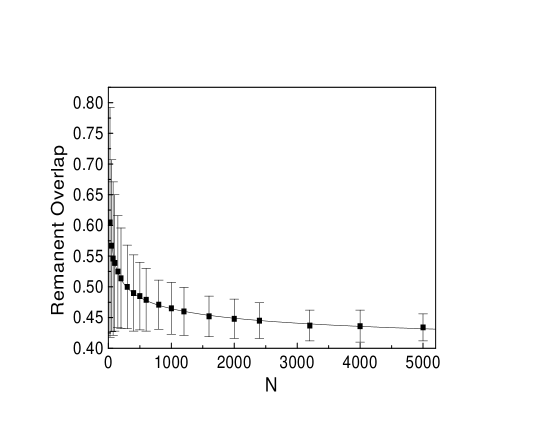
Figure 1: Remanent overlap for the even time dynamics obtained by numerical simulation for $J_{0}=0.8$, $\eta=1$, $m_{0}=1$ and various values of the network size $N$. The full curve denotes the best fit of the results to the form of Eq. (36).

We show in Fig. 2 the remanent overlap $m_{\infty}$ and the exponent $a$ of the power law decay of the even time dynamics in Eq. (35) as functions of $J_{0}$. The plots show clear evidence for a “transition” near $J_{0}=1$: the rate of increase of the remanent overlap $m_{\infty}$ with increasing $J_{0}$ is maximum near $J_{0}=1$, and the exponent $a$ has a minimum at the same value of $J_{0}$. This “transition” is from spin-glass-like to ferromagnet-like behaviour. The “spin-glass” phase for $J_{0}<1$ has a small value of the remanent overlap, arising due to the non-ergodic relaxation of the system through a complex energy landscape, which prevents it from reaching the equilibrium state corresponding to $m=0$. The system gets frozen to a cycle of length two which can be characterized by the remanent overlaps $m_{\infty}^{\rm even}$ and $m_{\infty}^{\rm odd}$ of the even and odd time dynamics, respectively. (Wherever we discuss the even time dynamics alone, we drop the superscript. Thus, $m_{\infty}^{\rm even}$ and $m_{\infty}$ both refer to the remanent overlap for the even time dynamics). For $J_{0}=0$, $m_{\infty}^{\rm even}=0.186\pm 0.001$ whereas $m_{\infty}^{\rm odd}=0$ (precisely, $O(10^{-3})$ which is the inherent level of errors involved in the calculation). Both of the remanent overlaps increase with $J_{0}$. Coming back to the even time dynamics we find in Fig. 2(b) that the relaxation becomes slower as $J_{0}$ is increased in the spin-glass phase. On the other hand, in the “ferromagnetic” phase ($J_{0}>1$), the system relaxes faster for higher value of $J_{0}$. The behavior is consistent with the physical intuition that $J_{0}$ is the strength of the ferromagnetic coupling which opposes the decay of the system to a small value of $m_{\infty}$ in the spin glass phase, while helping the system to have a large $m_{\infty}$ in the ferromagnetic phase.

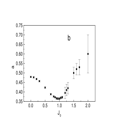
Figure 2: Results of fitting the mean-field Monte Carlo data for the evolution of the overlap, $m(t)$, at even times to Eq. (35) for $\eta=1$ and $m_{0}=1$. (a) Remanent overlap $m_{\infty}$ as a function of the acquisition strength $J_{0}$. (b) The exponent $a$ of the power law as a function of $J_{0}$.

We should emphasize that the “transition” mentioned above reflects a qualitative change in the short-time dynamical behavior of the system – it does not necessarily correspond to a phase transition in the thermodynamic sense. It is, however, interesting that the value of $J_{0}$ where this change in the dynamics occurs is consistent with the phase diagram of the SK model with ferromagnetic interactions [32], obtained by the replica theory, which shows a transition from the spin-glass phase to a ferromagnetic phase (with replica symmetry broken) at $J_{0}=1$.

Strictly speaking, the stored pattern is not absolutely stable for any finite value of $J_{0}$: the remanent overlap $m_{\infty}$ is always less than unity. However, this does not prevent the network from performing as an associative memory. For sufficiently large values of $J_{0}$, we can have $m_{\infty}$ very close to unity (e.g., for $J_{0}=2.0$, $m_{\infty}=0.942\pm 0.001$). $m_{\infty}$ can be made as close to unity as we wish by increasing $J_{0}$. A similar scenario exists in the Hopfield model, where for extensive loading of memory, the stored patterns are not fixed points of the dynamics. In the Hopfield model, too, we have retrieval fixed points which can be made closer to the respective stored patterns by reducing the memory loading level of the network. What matters in both the models is the ratio of the strengths of the signal and the noise terms in the expressions for the local fields. This substantiates the analogy of $J_{ij}^{\rm s}$ with the noise arising from stored patterns other than the one under retrieval in the Hopfield model.

As mentioned earlier, the synchronous dynamics, in general, takes the system to a limit cycle of length 2. For the network to function as an associative memory, it is desirable that the values of the overlap to which the network settles down at even and odd times are not very different. In Fig. 3 we plot together $m_{\infty}^{\rm even}$ and $m_{\infty}^{\rm odd}$ as functions of $J_{0}$. It is evident that for the values of the acquisition strength that are of interest ($J_{0}>1$), the difference between the two remanent overlaps are very nominal. We, therefore, concentrate only on the even time dynamics hence after.

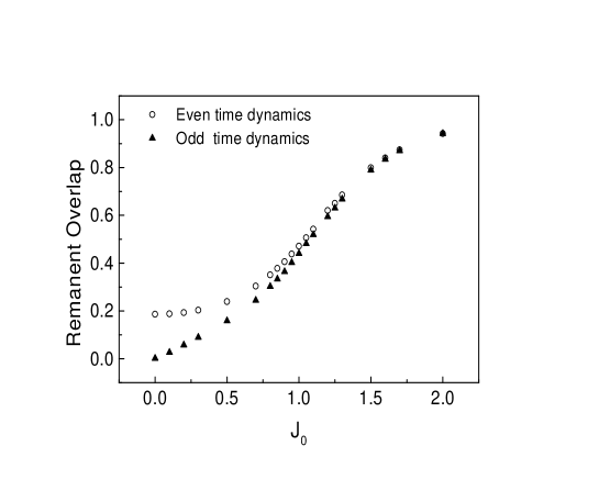
Figure 3: Remanent overlaps for the even-time and odd-time dynamics as functions of the acquisition strength $J_{0}$ for $\eta=1$ and $m_{0}=1$.

For the network to function as an associative memory, it also desirable that the attractor (limit cycle) corresponding to the stored pattern has a large basin of attraction, i.e., a large number of initial configurations having a finite overlap with the stored pattern (i.e., with $m_{0}\neq 0$) should converge to this attractor. We, therefore, have studied the dynamics of the system with $m_{0}=0.05$, which is well below the remanent overlap for all values of $J_{0}$. We find that $m(t)$ increases with time if $J_{0}>1$, decreases with time if $J_{0}<1$, and remains nearly constant for $J_{0}=1$. This behavior, shown in Fig. 4, also suggests a transition at $J_{0}=1$. Even for the values of $J_{0}>1$, two different kinds of behavior of $m(t)$ are possible. For relatively smaller values of $J_{0}$, the value of $m_{\infty}$ depends on the initial overlap $m_{0}$, e.g., for $J_{0}=1.3$ the values of $m_{\infty}$ for $m_{0}=0.05,\,0.3,{\rm and}\quad 0.5$ are quite different, as shown in Fig. 5, indicating the presence of different “attractors” (other than the one corresponding to the stored pattern) with their basins of attraction. Thus we have a complex phase-space structure for such values of $J_{0}$. This is consistent with the known result [32] that the zero-temperature ferromagnetic phase of the SK model is glassy with broken replica symmetry. On the other hand, for larger values of the acquisition strength, e.g. for $J_{0}=2$, different initial values of $m$ converge to the same $m_{\infty}$, indicating a relatively simple structure of the phase space. In Fig. 6 we show the evolution of $m$ for initial overlaps ranging from $m_{0}=0.005$ to $m_{0}=1$ for $J_{0}=2$. Since the initial overlap $m_{0}=0.005$ is already very close to the estimated value of $\Delta m=0.001$, it appears that all initial configurations with nonzero $m_{0}$ converge to the same attractor that corresponds to the stored pattern. Such a large basin of attraction for sufficiently high values of the acquisition strength may be an artifact of the one pattern model. In the case of many stored patterns, the size of the basin of attraction of one of the patterns would get reduced. However, the simple one-parameter model brings out the essential feature that it is possible to tailor the size of the basin of attraction of a stored pattern by varying the corresponding acquisition strength. Note that our result for a simple phase-space structure for large values of $J_{0}$ applies only to the subspace of states with finite values of $m$. It does not preclude the occurrence of a complex phase-space structure in the large subspace of states with zero magnetization.

Figure 4: Evolution of the overlap $m(t)$ at even times for different values of $J_{0}$ for $\eta=1$ and $m_{0}=0.05$.

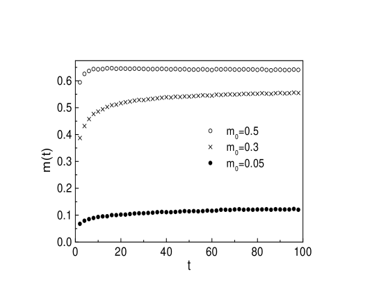
Figure 5: Evolution of the overlap $m(t)$ at even times for different values of $m_{0}$, the initial overlap with the stored pattern. The plots are for $\eta=1$ and $J_{0}=1.3$.

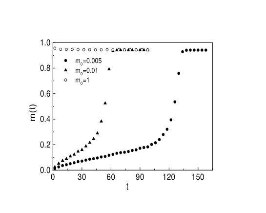
Figure 6: Same as Fig. 5 for $J_{0}=2$.

As mentioned earlier, the convergence time, which is the time taken by the network to reach the attractor corresponding to the stored pattern from an initial state in the basin of attraction of the attractor, is an important parameter in characterizing the performance of the network as an associative memory. From studies of spin-glass models, it is known that the dynamics for $\eta=1$ may become very slow, especially for small values of the initial overlap $m_{0}$ [33]. We also find evidence for slow dynamics in our calculations. For example, in Fig. 7 we show $m(t)$ for $J_{0}=1.5$ and $m_{0}=0.05$. Even at $t=350$, $m(t)$ does not show any sign of saturation. As there is no definite trend in the behavior of $m(t)$, it is not possible to predict the value of $m_{\infty}$ and the corresponding time scale.

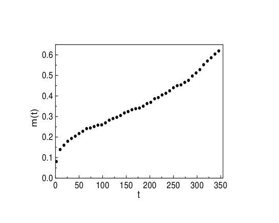
Figure 7: Evolution of the overlap $m(t)$ at even times for $J_{0}=1.5$, $\eta=1$ and $m_{0}=0.05$.

4.2 Asymmetric Couplings: $\eta<1$

As in the case of $\eta=1$, we first look at the effect of asymmetry in the couplings (by lowering the value of $\eta$) on the dynamics with the initial condition $m_{0}=1$. We find that the nature of relaxation changes from a pure power law to a combination of an exponential and a power law for $\eta<\eta_{c_{1}}$. Accordingly, the results of simulations can be fitted very well by the function

$$m(t)=m_{\infty}+\mathrm{const}\times t^{-a}\exp(-t/\tau)\,.$$ (37)

Thus for $\eta<\eta_{c_{1}}$, the overlap decays rapidly to $m_{\infty}$ with a finite relaxation time $\tau$. This behavior has also been reported in Ref. [15] for $J_{0}=0$. In that study, the remanent overlap $m_{\infty}$ was found to vanish at the same value of $\eta$, and the value of $\eta_{c_{1}}$ was found to be 0.825. For $J_{0}\neq 0$, we find both quantitative and qualitative deviations in the behavior of $m(t)$ from those reported in Ref. [15]. The value of $\eta_{c_{1}}$ increases beyond 0.825 as $J_{0}$ is increased from zero. For example for $J_{0}=1.5$, we have exponential relaxation for values of $\eta$ as high as 0.95. This is shown in Fig. 9. Moreover, $m_{\infty}$ vanishes for $\eta<\eta_{c_{2}}<\eta_{c_{1}}$. It is only at $J_{0}=0$ that $\eta_{c_{2}}=\eta_{c_{1}}$. The value of $\eta_{c_{2}}$ decreases as $J_{0}$ is increased. For example, for $J_{0}=0.8$, $\eta_{c_{2}}\simeq 0.65$ whereas for $J_{0}=1.5$ $\eta_{c_{2}}\simeq-0.2$. Furthermore, in the ferromagnetic phase, we find that over a considerable range of values of $\eta$, there is very little variation in the values of $m_{\infty}$, e.g. for $J_{0}=1.5$, $m_{\infty}$ varies from 0.80 to 0.72 when $\eta$ is reduced from 1 to 0. This feature of the network is highly desirable when the possibility of functional improvement is explored in the presence of asymmetry in the couplings. It ensures that the retrieval quality does not suffer significantly when $\eta<1$. When $J_{0}$ is sufficiently large, $m_{\infty}$ always remains close to unity, e.g., for $J_{0}=2$, $m_{\infty}$ varies 0.94 to 0.92 when $\eta$ is varied in its full range from 1 to $-1$.

Studies of models of spin glasses and neural networks suggest that the presence of asymmetry of an appropriate magnitude in the synaptic interaction matrix may result in the improvement of the performance of the network as an associative memory (see Ref. [16] for a detailed discussion on this aspect). It is expected that the asymmetry may destabilize some of the spurious attractors which do not correspond any stored pattern. If this happens, then the basin of attraction of the stored patterns would increase in size and the retrieval of memory would become faster. We find evidence of both of these effects. In Fig. 8, we show the evolution of the overlap $m(t)$ for various values of initial overlap ranging from $m_{0}=0.01$ to $m_{0}=1$ for $J_{0}=1.3$ and $\eta=0.6$. It can be easily seen that all these initial states converge to the same attractor with $m_{\infty}\simeq 0.56$. This signifies a considerable enhancement in the size of the basin of attraction when we compare this behaviour with that in Fig. 5. Note, however, that the retrieval quality has degraded in the model with synaptic asymmetry: the attractor corresponding the stored pattern has 68$\%$ overlap with the pattern for $\eta=1$ compared to the $\simeq 56\%$ overlap for $\eta=0.6$.

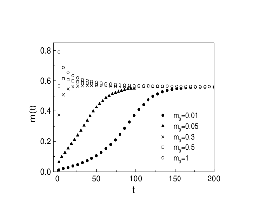
Figure 8: Evolution of the overlap $m(t)$ at even times for different values of $m_{0}$ in a network with $\eta=0.6$ and $J_{0}=1.3$.

In Fig. 9, we plot $m(t)$ for $J_{0}=1.5$ and $m_{0}=0.1$ for various values of the asymmetry parameter $\eta$. It is very clear that the retrieval of memory becomes faster as the asymmetry in couplings is increased. By fitting $m(t)$ with the function given in Eq. (37), we find that the time constant $\tau$ reduces from 55.56 to 4.61 when $\eta$ is varied from 0.95 to 0.6. At the same time, the value of the final overlap $m_{\infty}$ does not change much, indicating that the quality of retrieval is not substantially affected by the introduction of asymmetry in the synaptic interactions.

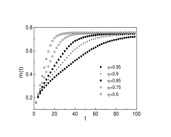
Figure 9: Evolution of the overlap $m(t)$ at even times for different values of $\eta$. The initial overlap $m_{0}$ is 0.1 and $J_{0}=1.5$.

5 Conclusion and Discussions

To summarize, we have studied the synchronous dynamics of a one-pattern model of associative memory using a mean field Monte Carlo method. Though simple, the model embodies sufficient richness to be useful in predicting the behavior of some of the more complicated models of associative memory such as the asymmetric Hopfield model. The two relevant parameters in the model are the acquisition strength $J_{0}$ of the stored pattern and the symmetry parameter $\eta$. For symmetric couplings ($\eta=1$), we find evidence for a transition at $J_{0}=1$. For $J_{0}<1$, we have a spin glass phase in which the retrieval overlap with the stored pattern is small, arising from a “remanence effect” (non-ergodic relaxation of the system through a complex energy landscape). On the other hand, for $J_{0}>1$ we have a ferromagnetic phase where the retrieval overlap with the stored pattern increases rapidly with $J_{0}$ and becomes very close to unity. Values of $J_{0}\geq 1.3$ would be required for a reasonable retrieval of the memory. Inside the ferromagnetic phase, we find the existence of two types of phase-space structure in the subspace of states having nonzero overlaps with the stored pattern. For example, for $J_{0}=2$, we have a relatively simple phase-space structure where all initial states with a nonzero overlap with the stored pattern flow to the attractor corresponding to the stored pattern. In contrast, for $J_{0}=1.3$ there are many attractors with their own basins of attraction. We also find that the process of retrieval becomes very slow for small values of $m_{0}$. When random asymmetry is introduced in the couplings ($\eta<1$), we find that it results, in general, in better retrieval performance of the network by enhancing the size of the basin of attraction of the stored pattern, as well as by making the recall of memory significantly faster.

How do the results described above compare with those obtained for the Hopfield model with random asymmetric interactions [16, 18]? Numerical simulations in Ref. [18] have shown that the presence of asymmetry in the synaptic interaction matrix makes the convergence to spurious attractors slower. On the other hand, the convergence time for correct retrieval is only marginally increased in the presence of asymmetry. Thus, asymmetry in the synaptic interaction matrix enhances the performance of the Hopfield net as an associative memory by providing a way of discriminating between spurious and retrieval attractors by looking at the dynamics of the network. In the model studied here, the improvement in performance occurs in a more direct manner: the retrieval becomes faster in the presence of asymmetry in the synaptic interaction matrix. Furthermore, the simulation results of Ref. [18] show that the introduction of asymmetry in the synaptic interaction matrix does not cause any enhancement of the typical size of the basins of attraction of stored patterns in the Hopfield model. Here we do find an enhancement of the size of the basin of attraction of the stored pattern. However, this occurs for a very restricted range of values of the parameter $J_{0}$. These results may be indicative of the enlargement of the basin of attraction being a model specific feature. Confirmation of some of these issues by extending the method used here to the asymmetric Hopfield model and to other models using different learning rules would be most interesting. A somewhat straightforward generalization of the technique for the case of two stored patterns with different acquisition strengths would provide useful insights into how the storage of other patterns, e.g., in the Hopfield model, would modify the results described above. Furthermore, this method may also be useful in analysing the effect of asymmetry in the synaptic interaction matrix of models of short-term memory [17, 34].

References

- [1] D. J. Amit, Modeling Brain Functions (Cambridge University Press, Cambridge, 1989).
- [2] J. Hertz, A. Krogh, and R. G. Palmer, Introduction to the Theory of Neural Computation (Addison-Wesley, Redwood CA, 1991).
- [3] H. K. Janssen, Z. Phys. B 23, 377 (1976).
- [4] R. Bausch, H. K. Janssen, and H. Wagner, Z. Phys. B 24, 113 (1976).
- [5] P. C. Martin, E. D. Siggia, and H. A. Rose, Phys. Rev. A 18, 423 (1978).
- [6] C. de Dominicis and L. Peliti, Phys. Rev. B 18, 353 (1978).
- [7] H. Sompolinsky and A. Zippelius, Phys. Rev. Lett. 47, 359 (1981); Phys. Rev. B 25, 6860 (1982).
- [8] R. D. Henkel and M. Opper, J. Phys. A 24, 2201 (1991).
- [9] E. Gardner, B. Derrida, and P. Mottishaw, J. Phys. (France) 48, 741 (1987).
- [10] M. P. Singh, Proc. D. A. E. Solid State Phys. Symp. 40 C, 414 (1997).
- [11] M. P. Singh, Ph.D. thesis, DAVV, Indore (2003).
- [12] G. A. Kohring and M. Schreckenberg, J. Phys. I 1, 1087 (1991).
- [13] S. Kirkpatrick and D. Sherrington, Phys. Rev. Lett. 35, 1792 (1975); Phys. Rev. B 17, 4384 (1978).
- [14] H. Eissfeller and M. Opper, Phys. Rev. Lett. 68, 2094 (1992).
- [15] H. Eissfeller and M. Opper, Phys. Rev. E 50, 709 (1994).
- [16] M. P. Singh, C. Zhang and C. Dasgupta, Phys. Rev. E 52, 5261 (1995).
- [17] G. Toulouse, S. Dehaene, and J. P. Changeux, Proc. Natl. Acad. Sci. USA 83, 1695 (1986).
- [18] C. Zhang, C. Dasgupta and M. P. Singh, Neural Computation 12, 865 (2000).
- [19] T. L. H. Watkin and D. Sherrington, J. Phys. A 24, 5427 (1991).
- [20] A. C. C. Coolen, in Handbook of Biological Physics IV: Neuro-Informatics and Neural Modeling (Elsevier Science, Amsterdam, 2000).
- [21] W. Krauth, J.-P. Nadal, and M. Mezard, J. Phys. A 21, 2995 (1988).
- [22] B. Derrida, E. Gardner, and A. Zippelius, Europhys. Lett. 4, 167 (1987).
- [23] A. Crisanti and H. Sompolinsky, Phys. Rev. A 36, 4922 (1987); Phys. Rev. A 37, 4865 (1988).
- [24] H. Sompolinsky, A. Crisanti, and H. J. Sommers, Phys. Rev. Lett. 61, 259 (1988).
- [25] H. Gutfreund, J. D. Reger and A. P. Young, J. Phys. A 21, 2775 (1988).
- [26] M. Bauer and W. Martienssen, J. Phys. A 24, 4557 (1991).
- [27] K. Nutzel, J. Phys. A 24, L151 (1991).
- [28] A. Crisanti, M. Falcioni, and A. Vulpiani, J. Phys. A 26, 3441 (1993).
- [29] U. Bastolla and G. Parisi, cond-mat/9803224 and references therein.
- [30] C. de Dominicis, Phys. Rev. B 18, 4913 (1978).
- [31] P. Hänggi, Z. Phys. B 31, 407 (1978).
- [32] K. H. Fischer and J. A. Hertz, Spin Glasses (Cambridge University Press, Cambridge 1991).
- [33] M. Mezard, G. Parisi, and M. A. Virasoro, Spin Glasses and beyond (World Scientific, Singapore, 1987).
- [34] M. Mezard, J. P. Nadal, and G. Toulouse, J. Physique 47, 1457 (1986).