Roughness of stylolites: a stress-induced instability with non local interactions

Abstract

We study the roughness of stylolite surfaces (i.e. natural pressure-dissolution surfaces in sedimentary rocks) from profiler measurements at laboratory scales. The roughness is shown to be nicely described by a self-affine scaling invariance. At large scales, the roughness exponent is $\zeta_{1}\approx 0.5$ and very different from that at small scales where $\zeta_{2}\approx 1.1$. A cross-over length scale at around $\lambda_{c}=1$mm is well characterized and interpreted as a possible fossil stress measurement if related to the Asaro-Tiller-Grinfeld stress-induced instability. Measurements are consistent with a Langevin equation that describes the growth of stylolite surfaces in a quenched disordered material with long range elastic correlations.

Stylolites are geological patterns that are very common in polished marbles, a material largely used for floors and walls of buildings and monuments. They exist in many sedimentary rocks such as limestones, sandstones or evaporites Bathurst71 . They are rock-rock interfaces, that are formed during diagenesis and result from combined stress-induced dissolution and precipitation processes Dewers90 ; Ortoleva94 ; Park68 . They exist on a very large range of scales, from micro-meters to tens of meters. They are often observed as thin irregular interfaces that look like printed lines on rock cuts which explain their name. At larger scales, they are planar structures that are typically perpendicular to the tectonic load (i.e. lithostatic pressure). They might form complex network with or without connections.

However, despite their abundance, stylolites are as mentioned by Gal et al. Gal98 “among the least well-explained of all pressure-solution phenomena”. First they are complex 3D structures that are often only described from 2D cross-sections. Second, they develop in various petrological and tectonic contexts which lead to very different geometries. Third they are often transformed and deformed because of post-processes like diagenesis and metamorphism that develop after their initiation.

In this letter we propose a new mechanism for stylolites growth that is consistent with recent 3D roughness measurements of a stylolite interface. The first part of the letter deals with the topography measurement and its description in terms of scaling invariance, namely self-affinity. The second part is devoted to a physical model of the stylolites roughening. It is based on a Langevin equation that accounts for a stress-induced instability in a quenched disorder with capillary effects and long range elastic interactions.

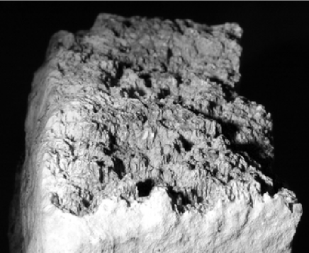
Figure 1: Picture of the stylolite surface that has developed in a limestone from Juras Mountains (France). Magnitude of the peaks are typically of the order of 2 mm. The width of the sample is 4 cm.

The roughness measurement has been performed on a stylolite interface included in a limestone sample from Juras Mountains in France (see Fig. 1). The sample has been collected in a newly open quarry, thus preserved from late breakage and chemical erosion. The opening procedure was possible for this sample because of the accumulation of undissolved minerals like clays that form a weak layer along the stylolite interface. The concentration of these minerals provides an estimate of the cumulative strain that the sample has undergone Renard03 . As shown in Fig. 1, peaks along the interface are randomly distributed in space and of various sizes (up to several millimeters). Locally slopes along the topography might be very important which makes the roughness measurement difficult.

Figure 2: A 1D profile obtained by a mechanical profiler (1030 data points - $\Delta x=30\mu$m).

We used two different profilers to sample the stylolite roughness. First, with a mechanical profiler Schmittbuhl95 ; Lopez98 we extracted four profiles of 1030 points each with a horizontal step of $\Delta x=30\ \mu$m. The specificity of the mechanical profiler is to measure the surface height from the contact of a needle onto the surface. The radius of the needle tip is 25 $\mu$m. The vertical resolution is $3\ \mu$m over the available range of 5 $cm$. One of this profile is shown in Fig. 2. We compare the mechanical measurement to an optical profiling Meheust02 . This technique is based on a laser triangulation of the surface without any contact with the surface. The laser beam is $30\ \mu$m wide. Horizontal steps between measurement points were $\Delta x=\Delta y=50\ \mu m$. The main advantage of this technique is the acquisition speed that can be significantly larger compared to the mechanical profiler since there is no vertical move. However, a successful comparison with mechanical measurement is necessary to ensure that optical fluctuations are height fluctuations and not material property fluctuations.

Fig. 3 shows a gray level map of the stylolite surface heights as a high resolution image ($600\times 600$ pixels) that covers over a surface area of 3$\times$3 cm². The vertical resolution is $2\ \mu$m over the $6$ mm vertical range of the setup.

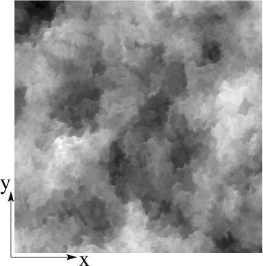
Figure 3: 2D map obtained by an optical profiler (600$\times$600 data points - $\Delta x=\Delta y=50\mu$m). Heights are gray encoded: white corresponds to the minimum height and black to the maximum height.

We analyzed the height distribution in terms of self-affinity Barabasi95 which states that the surface remains statistically unchanged for the transform: $\Delta x\rightarrow\lambda\;\Delta x$, $\Delta y\rightarrow\lambda\;\Delta y$, $\Delta z\rightarrow\lambda^{\zeta}\;\Delta z$, where $\lambda$ can take any real value. The exponent $\zeta$ is the so-called roughness exponent. A 1D Fourier spectrum of a self-affine profile is shown Barabasi95 to behave as a power law with a slope $-1-2\>\zeta$, and provides an estimate of the roughness exponent $\zeta$. We applied this technique whose reliability has been tested Schmittbuhl95b , to profiles extracted from the optical map shown in Fig. 3, either along $x$ or $y$ directions. Results are plotted in Fig. 4. The figure shows with a thick solid line the $y$-direction average spectrum of 600 profiles extracted along the $x$-direction. The spectrum clearly exhibits two regimes. At small wavenumbers (i.e. large length scales), a power law behavior is observed with a slope in the log-log plot of -2 which is consistent with a roughness exponent of $\zeta_{1}=0.5$. At large wavenumber (i.e. small length scales), a second power law behavior is observed with a larger slope (-3.2) in agreement with a roughness exponent $\zeta_{2}=1.1$. The crossover length scale is sharp and defines a characteristic length scale $\lambda_{c}\approx 1$mm. The average spectrum of profiles taken along the perpendicular direction ($y$-direction) provides a very consistent result and confirms the isotropy of the surface in terms of scaling invariance. We checked in Ref. Renard03 that mechanical profiles show the same properties specially at large wavenumbers since they are sampled at a higher resolution and allow an extended description of the unusual high roughness exponent $\zeta_{2}=1.1$. We also checked that another analysis technique, namely the Average Wavelet Coefficient technique Simonsen98 , was providing very consistent results. We also show in Ref. Renard03 that this behavior can be observed in several other stylolite samples. The difference between samples comes from the crossover length scale that can be larger or smaller, changing drastically the aspect of the surface. However, the two power law behaviors are conserved with the same values of the roughness exponents.

Figure 4: Averaged power spectrum of the topographic profiles extracted from the optical map of the stylolite surface.

The second part of the letter is devoted to a modeling of the stylolite roughening in order to understand the origin of the self-affine behaviors and the parameter sensitivity of the characteristic length $\lambda_{c}$. As usually done, we reduce the problem to a 2D situation $z(x)$, i.e. invariance along the $y$-direction.

We propose a phenomenological approach that follows the work reported in Kassner et al. Kassner01 who studied the dynamics of a strained solid in contact with its melt and more specifically the Asaro-Tiller-Grinfeld instability. In the case of a solid/fluid interface, the chemical potential between the solid and the fluid at the boundary can be written as Asaro72 ; Gal98 :

$$\Delta\mu=\Omega(u_{e}+\gamma\kappa)$$ (1)

where $u_{e}$ is the elastic energy per unit volume in the solid, $\gamma$ is the surface energy, $\kappa$ the curvature and $\Omega$ a molecular volume. We have assumed that gravity effects are negligible. If a bulk diffusion holds in the fluid, the evolution of the interface is directly related to the chemical potential: $v_{n}=m\Delta\mu$ where $v_{n}$ is the normal velocity and $m$ is the mobility.

Following the work of Grinfeld and Hazzledine Grinfeld96 , we propose to extend the approach to the case of a solid/solid interface. Moreover, we shall also assume the presence of a fluid in the pores. Porosity of the material is supposed to be sufficiently high for having both a bulk diffusion in the fluid and capillary effects. Doing so, Eq.(1) holds. Since a complete match between both solid surfaces is assumed, the normal velocity of the interface is now driven by the relative dissolution between the two solids.

The difficult task is to expand the local elastic energy along the interface that takes into account the surface corrugations. Using the representation theorem for the displacement field and the Hook’s law, it is possible to include the influence of non local elastic interactions in the limit of small perturbations of the interface through the elastic Green function as Bilby68 ; Gao89 :

$$\sigma(x)=\sigma_{0}\left(1+\frac{1}{2\pi}PV\int_{-\infty}^{\infty}{\frac{z(x^{\prime})-z(x)}{(x^{\prime}-x)^{2}}dx^{\prime}}\right)$$ (2)

where $\sigma(x)$ is the local stress along the interface between the solid, $\sigma_{0}$ is the average uniaxial external stress or an effective stress that includes the fluid pressure, and $PV$ is the principal value. According to Ref. Kassner01 , the elastic energy can be approximated for plain strain by:

$$u_{e}\approx\frac{(1-\nu^{2})}{E}\sigma^{2}(x)$$ (3)

where $E$ is an effective Young’s modulus and $\nu$ an effective Poisson coefficient.

The last aspect of the modeling concerns a description of the noise that exists in the chemical potential because of material fluctuations. We assume that this noise fluctuates on scales significantly smaller than the scales where elasticity and capillary effects are considered as for a Langevin approach Barabasi95 . However, unlike classical use of a Langevin equation, we assume here that the noise $\eta(x,z(x))$ is quenched to represent spatial material fluctuations, and known to have a strong influence on the scaling properties. For instance, for the Edwards and Wilkinson (EW) problem Edwards82 ; Roux94 , the roughness exponent is 0.5 in the case of an annealed noise and 1.2 for a quenched noise.

In the present framework, the interface evolution is described by the following equation:

$$\frac{1}{m}\frac{dz}{dt} = \Omega\frac{(1-\nu^{2})}{E}\sigma_{0}^{2}\left(1+\frac{1}{\pi}PV\int_{-\infty}^{\infty}{\frac{z(x^{\prime})-z(x)}{(x^{\prime}-x)^{2}}dx^{\prime}}\right)$$ (4)

$$+\ \Omega\gamma\frac{d^{2}z}{dx^{2}}\ +\ \eta(x,z(x))$$

which includes three driving forces: the long range elastic interactions, the local capillary effect which has a stabilizing influence, and the noise fluctuations. A crossover length scale is obtained by the balance of the average elastic and capillary terms in Eq.(4) Kassner01 :

$$\lambda^{*}=\frac{\gamma E}{\sigma_{0}^{2}(1-\nu^{2})}$$ (5)

Typical values for limestones are $E=8\cdot 10^{10}$ N/m², $\nu=0.25$, and $\gamma=20$ J/m². If we consider a stress at 2 km depth ($\sigma_{0}=40$ MPa), we obtain $\lambda^{*}\approx 1$ mm. We propose that the $\lambda^{*}$ length scale is the crossover length scale $\lambda_{c}$ observed in Fig. 4.

Actually, the mechanical regime ($\lambda\gg\lambda_{c}$) and the capillary regime ($\lambda\ll\lambda_{c}$) have both been extensively explored but independently. Indeed, the capillary regime is nothing else than the EW problem in a quenched noise. Roux and Hansen Roux94 have shown in this case that the interface is self-affine with an exponent $\zeta_{2}\approx 1.2$. In the mechanical regime, Eq.(4) is reduced to the quasistatic propagation of an elastic line in a disordered material. This has been largely studied Schmittbuhl95c ; Ramanathan98 ; Rosso02 and the roughness exponent has been shown to be $\zeta_{1}\approx 0.4$.

We performed a numerical simulation of Eq.(4) using an even driven algorithm Schmittbuhl95c ; Schmittbuhl99 where there is no time evolution. The periodic interface is discretized in N=2048 cells. At start, the interface is flat. At each step, we are searching for the cell that exhibits the maximum speed $dz/dt$ according to Eq.(4). This cell is then advanced by a random amount $dz$ uniformly sampled in $[0,1]$. The local fluctuation of the chemical potential $\eta(x,z(x))$ is updated from a prescribed distribution chosen here to be uniform between $[0,1]$. Doing so, we are always dealing with the most unstable cell and let the interface grow there.

Figure 5: Averaged power spectrum of the topographic profiles obtained from the 2D stylolite modeling.

After a transient regime, we observed a stationary width of the rough interface that develops. The power spectrum of the interface position $P(k)$, averaged over 500 samples, is shown in Fig. 5. It reveals a behavior very similar to the stylolite measurements: A characteristic length scale defined as the cross-over between two power law regimes. The crossover length scale $\lambda^{\star}$ is controlled by the balance between the magnitude of the mechanical and capillary effects and is compared to the charateristic length scale $\lambda_{c}$. As expected, the mechanical regime with an exponent $\zeta_{1}\approx 0.4$, is dominating at small wavenumbers (i.e. large length scales). On the contrary, at large wave numbers, the capillary regime dominates with a roughness exponent close to $\zeta_{2}=1.2$. Roughness exponents obtained from the modeling are slightly different from the measurements. This might be explained by the dimension difference: experimental surfaces are full 3D interfaces, on the contrary the model is 2D. A complete 3D numerical modeling is on-going to account for this situation. However, 3D computations are much heavier because of the long delay to reach the stationary regime of the interface growth.

In conclusion, we presented a quantitative description of stylolite interfaces that is consistent with a model of interface growth. The experimental measurement is a high resolution profiling of a 3D stylolite topography. We show that the surface is self-affine but with two regimes. At small scales, the roughness exponent is unexpectedly high, $\zeta_{2}=1.1$, and consistent with a capillary dominated regime. At large scales, the stylolites morphology is controlled by mechanical effects, i.e. long range elastic stress redistribution. In this case the roughening is important with a low roughness exponent $\zeta_{1}=0.5$. The modeling is based on the description of a stress-induced instability previously reported as the Asaro-Tiller-Grinfeld instability. Such framework provides a prediction of a characteristic length $\lambda_{c}$ which is the crossover between the two scaling regimes. It is important for geological implications to note that the characteristic length $\lambda_{c}$ is very sensitive to the average stress $\sigma_{0}$. Indeed, a measurement of $\lambda_{c}$ from today roughness profiling could provide an estimate of the stress magnitude during the stylolite growth, that is, in the past. Thus stylolites could be considered as stress fossils.

We acknowledge D. Rothman, J. Rice, A. Lobkovsky, B. Evans, Y. Bernabé, B. Goffé, P. Meakin, and E. Merino for very fruitful discussions. This work was partly supported by the ACI “Jeunes Chercheurs” of the French Ministry of Education (JS), and the ATI of the CNRS (FR).

References

- (1) R. Bathurst, Carbonate sediments and their diagenesis (Elsevier, Amsterdam, 1971).
- (2) T. Dewers and P. Ortoleva, Geochimica et Cosmochimica Acta 54, 1609 (1990).
- (3) P. Ortoleva, Geochemical self-organization (Oxford University Press, Cambridge, USA, 1994).
- (4) W. Park and E. Schot, Journal of Sedimentary Petrology 38, 175 (1968).
- (5) D. Gal, A. Nur, and E. Aharonov, Geophysical Research Letters 25, 1237 (1998).
- (6) F. Renard et al., in preparation (unpublished).
- (7) J. Schmittbuhl, F. Schmitt, and C. Scholz, J. Geophys. Res. 100, 5953 (1995).
- (8) J. Lopez and J. Schmittbuhl, Phys. Rev. E 57, 6999 (1998).
- (9) Y. Méheust, Ph.D. thesis, University Paris 11, 2002.
- (10) A. Barabási and H. Stanley, in Fractal concepts in surface growth, edited by A. Barabási and H. Stanley (Cambridge University Press, Cambridge, 1995).
- (11) J. Schmittbuhl, J. Vilotte, and S. Roux, Phys. Rev. E 51, 131 (1995).
- (12) I. Simonsen, A. Hansen, and O. M. Nes, Phys. Rev. E 58, 2779 (1998).
- (13) K. Kassner et al., Phys. Rev. E 63, 036117 (2001).
- (14) R. Asaro and W. Tiller, Met. Trans. 3, 1789 (1972).
- (15) M. Grinfeld and P. Hazzledine, Phil. Mag. Lett. 74, 17 (1996).
- (16) B. A. Bilby and J. D. Eshelby, in Fracture, an advanced treatise (H. Liebowitz, Editors, Academic Press, New York, 1968), Vol. I, pp. 99–182.
- (17) H. Gao and J. R. Rice, ASME Journal of Applied Mechanics 56, 828 (1989).
- (18) S. Edwards and D. Wilkinson, Proc. Roy. Soc. A 381, 17 (1982).
- (19) S. Roux and A. Hansen, Journal de Physique I 4, 515 (1994).
- (20) J. Schmittbuhl, S. Roux, J. Vilotte, and K. Måløy, Phys. Rev. Lett. 74, 1787 (1995).
- (21) S. Ramanathan and D. Fisher, Phys. Rev. B 58, 6026 (1998).
- (22) A. Rosso and W. Krauth, Phys. Rev. E 65, 025101 (2002).
- (23) J. Schmittbuhl and J. Vilotte, Physica A 270, 42 (1999).