Field-tuned quantum tunneling in a supramolecule dimer [Mn₄]₂

Abstract

Field-tuned quantum tunneling in two single-molecule magnets coupled antiferromagnetically and formed a supramolecule dimer is studied. We obtain step-like magnetization curves by means of the numerically exact solution of the time-dependent Schrődinger equation. The steps in magnetization curves show the phenomenon of quantum resonant tunneling quantitatively. The effects of the sweeping rate of applied field is discussed. These results obtained from quantum dynamical evolution well agree with the recent experiment[W.Wernsdorfer et al. Nature 416(2002)406].

APCS Number: 75.50.Xx,75.45.+j,76.20.+q

The macroscopic quantum phenomena in molecular magnets has become a very attractive researching field. Many properties of these nanometer-sized magnetic particles and clusters, such as Mn₁₂($s=10$), Fe₈($s=10$) and Mn₄($s=\frac{9}{2}$) systems, have been well studied^[1]-[6] both experimentally and theoretically. Theoretically, studying the phenomenon of quantum resonant tunneling of these molecular magnets could be based on Landau-Zener (LZ) transitions^[7],[8], or based on numerically the solution of the time-dependent Schrődinger equation^[9],[10]. In Landau-Zener model, the magnetization curves could be obtained in a static and approximate way. Recently a supermolecular dimer [Mn₄]₂ is reported to be synthesized successfully by Werndorfer et al.^[11]. In this kind of supermolecular dimer, two single-molecule magnets Mn₄ antiferromagnetic coupled each other, which results in its quantum behavior quite different from two individual Mn₄ molecule without coupling. In this paper, we calculate magnetization curves of a supermolecular dimer [Mn₄]${}_{2},$a single-molecule magnets, by numerically exact solution of the time-dependent Schrődinger equation.

Following Wernsdorfer et al., the model Hamiltonian of the supermolecular dimer [Mn₄]₂ is

$$H=H_{1}+H_{2}+JS_{1}\cdot S_{2},$$ (1)

where $J$ is the weak antiferromagnetic supercharging coupling constant. H₁ and H₂ are Hamiltonian for two individual Mn₄ molecules in the supermolecular dimer. It is known that the model Hamiltonian of an individual Mn₄ molecule is

$$H_{i}=-DS_{zi}^{2}+E(S_{xi}^{2}-S_{yi}^{2})-g\mu_{B}S_{zi}h_{z}(t),i=1,2,$$ (2)

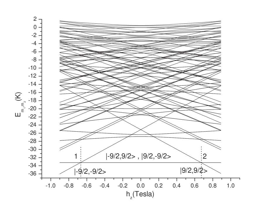
Figure 1: The 100 spin state energies of the model Hamiltonian(Equation (1)) as a function of longitude applied field. A weak transverse field $h_{x}=0.01Tesla$ is take into account.

where $D$ and $E$ are the axial anisotropic constants. $h_{z}(t)$ is the applied sweeping field along easy axis. We can easily obtain the energy eigenvalues of whole Hamiltonian $H$ (Figure 1). In experiment the sweeping rate of $h_{z}(t)$ is very slow, so we can simulate it as a step-increased field, which means the $h_{z}$ increases a value $\Delta h_{z}$ every $\tau$ time step and keeps constant during the $\tau$ time intervals. Note that we can not use a sweeping rate as slow as experiment due to the limitation of our computing time. However, we can obtain the key macroscopic quantum phenomena in our calculation with relatively high sweeping rate. In this paper, we select $D=0.72k,J=0.1k,$^[11]and $E=0.0317k$^[6]. Dynamic evolution follows time-dependent schrődinger equation and can be calculated by

$$\left|\Psi\left(t\right)\right\rangle=\left|\Psi\left(t_{0}+n\tau\right)\right\rangle=\exp[-iH(t_{0}+(n-1)\tau)\cdot\tau]\left|\Psi\left(t_{0}+(n-1)\tau\right)\right\rangle,$$ (3)

Meanwhile, $\left|\Psi\left(t\right)\right\rangle$ can be expanded as

$$\left|\Psi\left(t\right)\right\rangle=\overset{S}{\underset{m_{1}=-s}{\sum}}\overset{S}{\underset{m_{2}=-s}{\sum}}a_{m_{1},m_{2}}\left(t\right)\left|m_{1},m_{2}\right\rangle,S=\frac{9}{2},$$ (4)

where $\left|m_{1},m_{2}\right\rangle$ are the eigenstates of $H_{0}$ that is

$$H_{0}=-DS_{z1}^{2}-DS_{z1}^{2}+JS_{z1}\cdot S_{z2}-g\mu_{B}(S_{z1}+S_{z2})h_{z}(t),$$ (5)

We assume the initial states to be at $\left|-\frac{9}{2},-\frac{9}{2}\right\rangle$, and the whole evolution process can be obtained by equation (4) step by step. In Ref.^[11], Wernsdorfer report five points (Figure 4 of Ref.) of resonant tunneling that result in the steps in hysteresis loops. They considered the first point is caused by the resonant transition from $\left|-\frac{9}{2},-\frac{9}{2}\right\rangle$ to$\left|-\frac{9}{2},\frac{9}{2}\right\rangle$, and the fourth point is caused by those from $\left|-\frac{9}{2},-\frac{9}{2}\right\rangle$ to$\left|-\frac{9}{2},\frac{5}{2}\right\rangle$. However, under the model Hamiltonian of Equation(1) and Equation(2), the transitions of these points are quenched for a half integer spin due to the parity symmetry^[12],[13]. Therefore, there must be some kind of transverse field components resulted from the influence of the environmental degrees^[6], such as hyperfine and dipolar couplings, and it can be approximated a Gaussian distribution with a width $\sigma=0.035T$ for such additional transverse environmental field. In this paper, we simply assume it to be a constant and $h_{x}=0.01T$ along x axis, but do not lose the essential physics, the macroscopic quantum phenomena.

The magnetization along the $z$ axis can be simply defined by $M=<S_{z1}+S_{z2}>$. In Figure 2, we plot the magnetization curve responding to a time-dependent applied field with a constant transverse field $h_{x}=0.01T$. There are three steps in the magnetization curve. In order to know the details of state transitions, the states ($\left|\Psi\left(t\right)\right\rangle$) near to two sides of resonant points are recorded in our simulation and they are shown in Table 1, where the occupied probabilities ($\left|a_{m_{1},m_{2}}\left(t\right)\right|^{2}$) are neglected to zeros if they less than $10^{-3}$. Therefore, we can get clear information of the process of evolution and transition. Figure 1 and Table 1 show that the first step occurs at $h_{z}=0.198T$ from $\left|-\frac{9}{2},-\frac{9}{2}\right\rangle$ to$\left|-\frac{9}{2},\frac{7}{2}\right\rangle$ (and$\left|\frac{7}{2},-\frac{9}{2}\right\rangle$), and the second step occurs at $h_{z}=0.731T$ from $\left|-\frac{9}{2},-\frac{9}{2}\right\rangle$ to$\left|-\frac{9}{2},\frac{5}{2}\right\rangle$ (and$\left|\frac{5}{2},-\frac{9}{2}\right\rangle$). These two resonant points fit well to experimental results (i.e. the point 2 and the point 4 of Fig.4 in Ref.^[11]). The third step occurs at $h_{z}=0.812T$ from $\left|-\frac{9}{2},\frac{5}{2}\right\rangle$ (and$\left|\frac{5}{2},-\frac{9}{2}\right\rangle$) to$\left|\frac{7}{2},\frac{5}{2}\right\rangle$ (or$\left|\frac{5}{2},\frac{7}{2}\right\rangle$). There is no step at $h_{z}\approx-0.33T$ in our magnetization curve, but the experiment reports a point of resonant tunneling (the point 1 in Fig.4 of Ref.^[11]). The reason is that we have used a too fast sweep rate in our simulation. We will interpret it more detail late. In our magnetization curve, since the step at $h_{z}\approx-0.33T$ from $\left|-\frac{9}{2},-\frac{9}{2}\right\rangle$ to$\left|-\frac{9}{2},\frac{9}{2}\right\rangle$ does not occur, therefore the step at $h_{z}=0.87T$ from $\left|-\frac{9}{2},\frac{9}{2}\right\rangle$ to$\left|\frac{7}{2},\frac{9}{2}\right\rangle$ (point 4 in the Fig.4 of Ref.^[11]) can not occur naturally.

In order to interpret why there is no step at $h_{z}=-0.33T$ in our magnetization curve, we firstly consider a utmost-slow process. At any $t$ value, the eigenstates and eigenvalues (Figure 1) of whole Hamiltonian $H(t)$ can be calculated by

$$H(t)\left|\Phi(E)\right\rangle=E\left|\Phi(E)\right\rangle,$$ (6)

Note that no matter how weak it is, the system always interact with environment which cause dissipation. Therefore, in a very very slow process, we can assume that the state $\left|\Psi(t)\right\rangle$ of system evaluating from a initial state $\left|\Psi(0)\right\rangle$ will always relax to the ground state $\left|\Phi(E_{\min})\right\rangle$ of $H(t)$. Figure 3 shows the magnetization curve of this utmost-slow process. There are two steps at $h_{z}\approx-0.3363T$ and $h_{z}\approx 0.3363T$ in the curve. It means that the point of resonant tunneling at $h_{z}\approx-0.3363T$ (point 1 of Fig.4 of Ref.^[11]) occurs when the sweeping rate of applied field is very slow. In figure 2, the sweeping rate of applied field in our calculation is $c=\frac{\Delta h_{z}}{\tau}=\frac{10^{-5}}{10^{-8}}=1000$ $Tesla/s$, which is much more larger than the ones in experiment ($0.140$ $Tesla/s$, $0.035$ $Tesla/s$ and $0.004Tesla/s$)^[11]. Due to the limitation of our computer time, we can not do the calculation for a sweeping rate of applied field as slow as the one in experiment. We now try to simulate the magnetization process (Figure 4) only in a very sharp range of $h_{z}$ with sweeping rates as slow as the ones used in experiment. In our figure 4, (a) is calculated over a range of $h_{z}$ from $-0.3364$ $Tesla$ to $-0.3362$ $Tesla$ with parameters $\tau=10^{-8}s$ and $\Delta h_{z}=10^{-9}Tesla$ (the sweeping rate $\sim 0.10$ $Tesla/s$); (b) is calculated over a range of $h_{z}$ from $-0.336295$ $Tesla$ to $-0.336275$ $Tesla$ with parameters $\tau=10^{-8}s$ and $\Delta h_{z}=10^{-10}$ $Tesla$ ( the sweeping rate $\sim 0.01Tesla/s$); (c) is the combination of (a) and (b). A very clear step occurs at $h_{z}\approx-0.336283T$ point, and it shows that the slower sweeping rate induces the higher step occurred. The recorded states (Table 2) at transition point $h_{z}\approx-0.3363$ $Tesla$ show that the resonant tunneling is from $\left|-\frac{9}{2},-\frac{9}{2}\right\rangle$ to$\left|-\frac{9}{2},\frac{9}{2}\right\rangle$ (and$\left|\frac{9}{2},-\frac{9}{2}\right\rangle$). All these results fit well with the results of experiment^[11]. Therefore, it clear show that the reason for no step at point about $h_{z}\approx-0.3363Tesla$ is from too fast sweeping rate of the applied field in theoretical simulation. There are some small oscillations in the magnetization curve. It is caused from quantum fluctuations.

In conclusion, We have studied the phenomenon of quantum resonant tunneling in a supermolecular dimer [Mn₄]₂ of single-molecule magnets by numerically exact solution of the time-dependent Schrődinger equation. We obtain step-like magnetization curves which demonstrate quantum tunneling quantitatively. We have calculated and discussed the affect to steps caused by different sweeping rate of applied field. It shows that some steps can not occur at some resonant points when the sweeping rate is too fast, but they could appear when the sweeping rate becomes enough slow. At a very narrow region near resonant point, we slow down the sweeping rate of applied field, some quantum resonant tunnelling appeared in experiment can appear. Meanwhile, theoretical calculation show that more slow rate induces more higher transition step. The results of our calculation fit very well with the experiment^[11]. Note that since we do not take into account the effects of dissipation caused by environment, the magnetization curves we obtain can not reach a reversal saturation value even if the applied field increase to infinitive value. Therefore, if we want to calculate a whole hysteresis loop, a proper mechanism of dissipation should be taken into account.

This work is supported by National Natural Science Foundation of China.

caption

Table1: Occupied probabilities $\left|a_{m_{1},m_{2}}\left(t\right)\right|^{2}$ at spin states $\left|m_{1},m_{2}\right\rangle$ (Equation (5)) at some points of the evolution process (Figure 2). The values are neglected to zero if they are smaller than $0.001$.

$h_{z}(Tesla)$	-0.34	-0.32	0.19	0.21	0.72	0.74	0.80	0.82	0.9
$\left|-\frac{9}{2},-\frac{9}{2}\right\rangle$	0.9986	0.9987	0.9987	0.9861	0.9855	0.9719	0.9718	0.9718	0.9717
$\left|-\frac{9}{2},\frac{7}{2}\right\rangle$	0	0	0	0.0062	0.0061	0.0060	0.0062	0.0061	0.0060
$\left|\frac{7}{2},-\frac{9}{2}\right\rangle$	0	0	0	0.0062	0.0061	0.0060	0.0062	0.0061	0.0060
$\left|-\frac{9}{2},\frac{5}{2}\right\rangle$	0	0	0	0	0	0.0068	0.0067	0.0053	0.0053
$\left|\frac{5}{2},-\frac{9}{2}\right\rangle$	0	0	0	0	0	0.0068	0.0067	0.0053	0.0053
$\left|\frac{7}{2},\frac{5}{2}\right\rangle$	0	0	0	0	0	0	0	0.0013	0.0013
$\left|\frac{5}{2},\frac{7}{2}\right\rangle$	0	0	0	0	0	0	0	0.0013	0.0013
$Total$	0.9986	0.9987	0.9987	0.9985	0.9977	0.9975	0.9977	0.9973	0.9970

Table2: Occupied probabilities $\left|a_{m_{1},m_{2}}\left(t\right)\right|^{2}$ at spin states $\left|m_{1},m_{2}\right\rangle$ (Equation (5)) at some points of the evolution process (Figure 4). The values are neglected to zero if they are smaller than $0.0001$.

Figure 4	(a)		(b)
$h_{z}(Tesla)$	-0.3364	-0.3362	-0.336295	-0.336275
$\left|-\frac{9}{2},-\frac{9}{2}\right\rangle$	1	0.9966	1	0.9679
$\left|-\frac{9}{2},\frac{9}{2}\right\rangle$	0	0.0016	0	0.0160
$\left|\frac{9}{2},-\frac{9}{2}\right\rangle$	0	0.0016	0	0.0160
$Total$	1	0.9998	1	0.9999

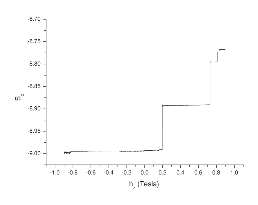
Figure 2: Magnetization relaxation of ground state (Magnetization curve reponse to a sweeping field. The sweeping rate is $c=\frac{\Delta h_{z}}{\tau}=\frac{10^{-5}}{10^{-8}}=1000Tesla/s$.

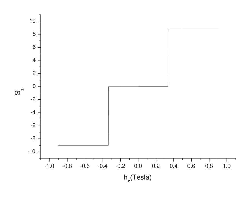
Figure 3: Magnetization curve based on a utmost-slow process. It suppose that the state $\left|\Psi(t)\right\rangle$ of system always relax to the ground state $\left|\Phi(E_{\min})\right\rangle$ of $H(t)$.

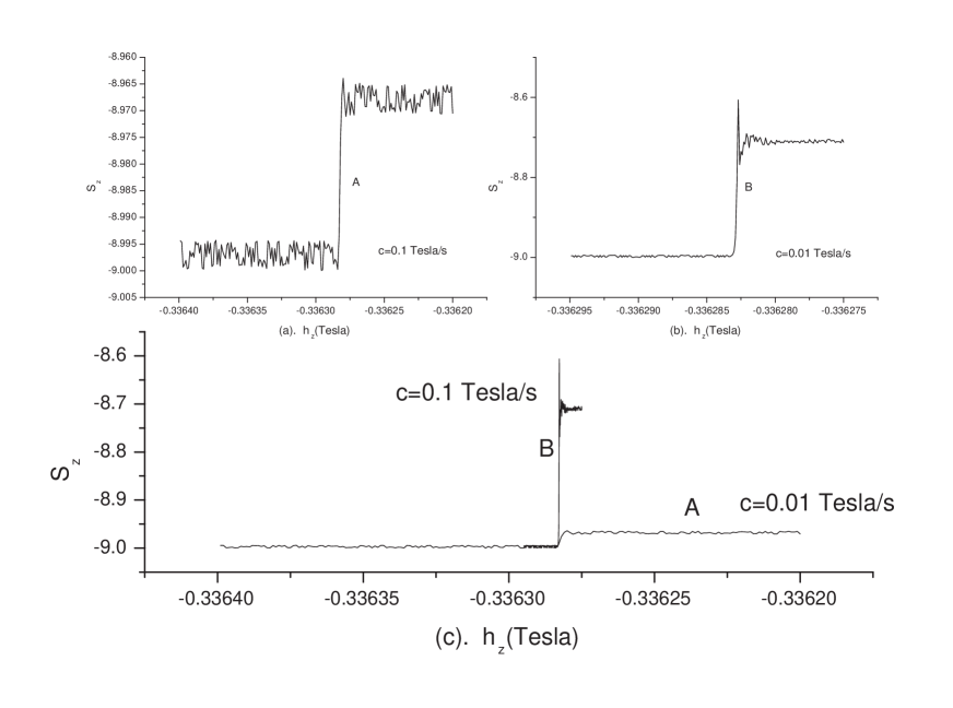
Figure 4: Magnetization curves response to slow sweeping fields over very sharp ranges of $h_{z}$. The sweeping rates are the same order with that used in experiment (Ref.^[11]).

References

- (1) L.Thomas, F.lionti, R.ballou, R.Sessoli, D.Gatteschi and B.Barbarra: Nature 383(1996)145.
- (2) P.C.E.Stamp: Nature 383(1996)125.
- (3) E.M.Chudnovsky: Science 274(1996)938.
- (4) J.R.Friedman, M.P.Sarachik, J.Tejada and R.Ziolo: Phys. Rev. Lett. 76(1996)3830.
- (5) W.Wernsdorfer and R.Sessoli: Science 284(1999)133.
- (6) W.Wernsdorfer, S.Bhaduri, C.Boskovic, G.Christou and D.N.Hendrickson: Phys. Rev. B 65(2002)180403.
- (7) C.Zener: Proc. R. Soc. London .Ser. A 137(1932)696.
- (8) H.De Raedt, S.Miyashita, K.Saito, D.Garcia-pablos and N.Garcia: Phys. Rev. B 56(1997)11761.
- (9) D.Garcia-Pablos, N.Garcia and H.De Raedt: J. Appl. Phys. 83(1998)6937.
- (10) E.Rastelli and A.Tassi: Phys. Rev. B 64(2001)064410.
- (11) W.Wernsdorfer, N.Allaga-Alcalde, D.N.Hendrickson and G.Christou: Nature 416(2002)406.
- (12) D.loss, D.P.Divincenzo and G.Grinstein: Phys. Rev. Lett. 69(1992)3232.
- (13) Jan von Delft and C.L.Henley: Phys. Rev. Lett. 69(1992)3236.