Scale-Free and Stable Structures in Complex Ad hoc networks

Abstract

Unlike the well-studied models of growing networks, where the dominant dynamics consist of insertions of new nodes and connections, and rewiring of existing links, we study ad hoc networks, where one also has to contend with rapid and random deletions of existing nodes (and, hence, the associated links). We first show that dynamics based only on the well-known preferential attachments of new nodes do not lead to a sufficiently heavy-tailed degree distribution in ad hoc networks. In particular, the magnitude of the power-law exponent increases rapidly (from $3$) with the deletion rate, becoming $\infty$ in the limit of equal insertion and deletion rates. We then introduce a local and universal compensatory rewiring dynamic, and show that even in the limit of equal insertion and deletion rates true scale-free structures emerge, where the degree distributions obey a power-law with a tunable exponent, which can be made arbitrarily close to -2. These results provide the first-known evidence of emergence of scale-free degree distributions purely due to dynamics, i.e., in networks of almost constant average size. The dynamics discovered in this paper can be used to craft protocols for designing highly dynamic Peer-to-Peer networks, and also to account for the power-law exponents observed in existing popular services.

I Introduction

Several random protocols (i.e., stochastic rules for adding/deleting nodes and edges) that lead to the emergence of scale-free networks have been recently proposed. The underlying dynamics for almost all of these models follow the principle of preferential attachment for targeting or initiating newly created links of the network. The simplest case is the linear preference for the target node of a new link: a node is added to the network at each time step, and the probability that a node $i$ with $k(i,t)$ links at time $t$ ($t>i$) receives a new link at time $t+1$, is $\propto k(i,t)$. The resulting network for this simple model has a power-law degree distribution with an exponent $|\gamma|=3$. Other variations of this procedure have also been widely studied Dog1 ; Krap ; BA ; chung .

The interesting properties of random power-law networks appear when the degree exponent $|\gamma|<3$. These properties include almost constant diameter and zero percolation threshold. Moreover, almost all cases of power-laws observed in real life networks, which these models ultimately might want to account for, have exponents less than $3$. Motivated by both these issues, a few stochastic linking rules resulting in exponents with magnitude less than $3$ have been introduced. Examples of such protocols include, the doubly-preferential attachment scheme for links, where both the initiator and the target nodes of an edge are chosen preferentially, as proposed in Dog3 ; chung , and the rewiring scheme of existing links to preferential targets as proposed in BB .

Most of these random protocols have been motivated by the need to model growing and mostly rigid networks, where nodes and links are gradually added. Examples of such graphs are the citation and collaboration networks. Once a connection is made between two nodes in these graphs it is never deleted and also nodes never leave the network. A second class of networks that has been studied is where the nodes are stable, but the links could be deleted. For example, on the WWW one can assume nodes to almost always remain in the network once created; however, existing links can easily be deleted, and new links created. In this paper, we primarily address a third class of networks (first introduced in Dog1 ), where the nodes themselves are also unstable and unreliable, and in an extreme case, the nodes (and hence all their connections) might leave the network without prior notice and through independent decisions. .

Our motivation for considering such dynamic networks comes, in part, from the recent interest towards less structured or ad hoc distributed system designs with peer-to-peer (P2P) content sharing networks as a prime example. In an instance of Gnutella, for example, a study GNUT shows that almost 80% of all nodes log-off within five hours from their log-in. Hence, the time scale within which the network assumes its structure is much shorter than the time scale within which it grows. A number of crawls of these networks show that at least in some regimes they follow a power-law. However, a stochastic model that can lead to the emergence of such complex networks has not been proposed. Another significant example is the ad hoc and mobile communication paradigms where each member can provide a short-time unreliable service and yet a global topological structure is to be ensured at all times.

We first use the continuous rate equation approach introduced in Dog1 (see Section II) to predict the power-law exponent for stochastic models, where new nodes joining the network make links preferentially, and existing nodes in the network are uniformly deleted at a constant rate. Contrary to previous claims Dog1 , we show that for such models the power-law degree distribution of the resulting network has an exponent $|\gamma|>3$, and that it rapidly approaches $-\infty$ as the deletion and insertion rates become equal. Thus a network with even small deletion rates will essentially have characteristics that are more similar to an exponential degree distribution. In Section III, we introduce our compensatory rewiring procedure, which is a novel way to exploit the deletion dynamic of the nodes itself to maintain a scale-free structure. In this protocol, in addition to the new nodes making preferential attachments, existing nodes compensate for lost links by initiating new preferential attachments. In fact, we show that the exponent of the power-law for the degree distributions of the resulting networks for any deletion rate, can be tuned as close to $-2$ as desired. Thus, our results provide a random protocol for generating scale-free networks even in the limit where the deletion and addition rates are equal and the network size is almost constant. To the best of our knowledge, this is the only procedure resulting in scale-free structures with exponent arbitrary close to $-2$ while the network size is almost constant.

These results can be applied for both analysis and design of complex networks (see Section IV). For example, our results provide an intuitive account for the existence of scale-free structures in many of the P2P networks GNUT . Perhaps, more significantly, our results provide a truly local protocol for generating highly dynamic scale-free and tunable networks. While such scale-free unstructured P2P networks have been thought to inherently suffer from scalability problems related to searching, our recent results prove this commonly-held notion to be false, and show that one can indeed perform searches in highly scalable fashion on such networks scalable . Thus, one could use the protocols introduced in Section III to design very active and efficiently searchable content sharing networks.

II Growing networks in the presence of permanent node deletion

The scale free properties of growing networks that incorporate preferential attachment with permanent deletion of randomly chosen links was considered by Dorogovtsev et al Dog1 . They concluded that the scale free properties of the emerging network depends strongly on the deletion rate of the links, and in fact the scale free behavior is observed only in low deletion rates. However, the analysis of the effect of random deletions of nodes at a fixed rate was incomplete. A correct analysis is presented in this section, and as noted in the introduction, the associated results are shown to have far-reaching consequences for ad hoc networks.

II.1 Preferential attachment and random node deletions

We consider the following model: at each time step, a node is inserted into the network and it makes $m$ attachments to $m$ preferentially chosen nodes. That is, for each of the links, a node with degree $k$ is chosen as a target with probability proportional to $k$. Then with probability $c$, a randomly chosen node is deleted.

We adopt the same approach as introduced in Dog1 for our analysis. Let each node in the network be labelled by the time it was inserted, and define $k(i,t)$ as the degree of the node inserted at time $i$ (i.e., the $i^{\hbox{th}}$ node) at time $t$. Let $D(i,t)$ be the probability that the $i^{\hbox{th}}$ node is not deleted (i.e., it is still in the network) until time $t$. Assuming the $i^{th}$ node to be in the network at time $t$, the rate at which its degree increases is:

$$\frac{\partial k(i,t)}{\partial t}=m\frac{k(i,t)}{S(t)}-c\frac{k(i,t)}{N(t)},$$ (1)

where

$$S(t)=\int_{0}^{t}D(i,t)k(i,t)di$$ (2)

is the sum over the degrees of all nodes that are present in the network at time $t$, and $N(t)=(1-c)t$ is the total number of nodes in the network. Note that the first term in Eqn. (1) is simply the number of links node $i$ receives as a result of the $m$ preferential attachments made by the newly introduced node. The probability that a randomly chosen node is among the neighbors of node $i$, and hence the probability that node $i$ loses a link, is of course, $\frac{k(i,t)}{N(t)}$, which accounts for the second term in Eqn. (1). We neglect all higher order effects.

Next, we solve the various unknown quantities in the following order: $D(i,t)$, $S(t)$, and then $k(i,t)$. First, using independence of the events corresponding to random deletions of nodes at each time step, it is easy to verify that $D(i,t+1)=D(i,t)(1-\frac{c}{N(t)})$. Hence, the continuous version of the dynamic of $D(i,t)$ can be stated as follows:

$$\frac{\partial D(i,t)}{\partial t} = -c\frac{D(i,t)}{N(t)}=-\frac{c}{1-c}\frac{D(i,t)}{t}\ .$$

Since, $D(t,t)=1$, we get

$$D(i,t)=\left(\frac{t}{i}\right)^{\frac{c}{c-1}}.$$ (3)

To find $S(t)$, we first multiply both sides of Eqn. (1) by $D(i,t)$ and integrate out $i$ from $0$ to $t$. Then,

$$\int_{0}^{t}D(i,t)\frac{\partial k(i,t)}{\partial t}di=m-c\frac{S(t)}{(1-c)t}.$$ (4)

The left-hand-side of the above equation can now be simplified as follows:

$$\int_{0}^{t}\frac{\partial}{\partial t}\{D(i,t)k(i,t)\}di-\int_{0}^{t}k(i,t)\frac{\partial}{\partial t}D(i,t)di =$$ (5)

$$\hbox{}\frac{\partial}{\partial t}\left[\int_{0}^{t}\{D(i,t)k(i,t)\}di\right]-k(t,t)D(t,t)-$$

$$\hbox{}\int_{0}^{t}k(i,t)\frac{c}{t(c-1)}D(i,t)di\ .$$

Substituting the above expression in Eqn. (4), and noting that $k(t,t)=m$ and $D(t,t)=1$, we get

$$\frac{\partial S(t)}{\partial t}-m-\frac{c}{(c-1)t}S(t)=m-c\frac{S(t)}{(1-c)t}\ .$$ (6)

The solution to the above equation is:

$$S(t)=2m\frac{1-c}{1+c}t=2m\frac{N(t)}{1+c}\ .$$ (7)

Since the correctness of this last equation is the key to further derivations and since this equation marks the departure from the results in Dog1 , we have paid especial attention to it. In particular, if we define the average degree of nodes at time $t$ as $\left\langle k(t)\right\rangle=\frac{S(t)}{N(t)}$, then Eqn. (7) implies that

$$\left\langle k(t)\right\rangle=\frac{2m}{(1+c)}=\left\langle k\right\rangle\ ,$$

i.e., the average degree of nodes is modified by a factor of $(1+c)$. Fig. 1 depicts the simulation results verifying the prediction of Eqn. (7).

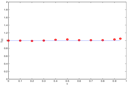
Figure 1: $T(c)=\left\langle k\right\rangle\frac{(1+c)}{2m}$ as a function of $c$, the deletion rate. Eqn. (7) predicts this quantity to be $1$ regardless of $c$. The simulation is for $m=7$, and $c$ ranges from $0$ to $0.95$, and the simulation time is $20000$ time steps.

Inserting Eqn. (7) back into the rate equation, we get:

$$\frac{\partial k(i,t)}{\partial t} = m\frac{(1+c)k(i,t)}{2m(1-c)t}-\frac{c}{1-c}\frac{k(i,t)}{t}$$

$$= \frac{(1+c-2c)k(i,t)}{2(1-c)t}=\frac{k(i,t)}{2t}\ ,$$

which implies that

$$k(i,t) = m(\frac{t}{i})^{\beta}\ ,$$ (8)

where $\beta=1/2$. Eqn. (8) is quite significant since it states that the degree of a node in the network (when it is not deleted), does not depend on the deletion rate. To verify this, we have made numerous simulations for a wide range of deletion rates. Fig. 2 shows the results for two rather extreme cases of 20% and 70% deletion rates, respectively.

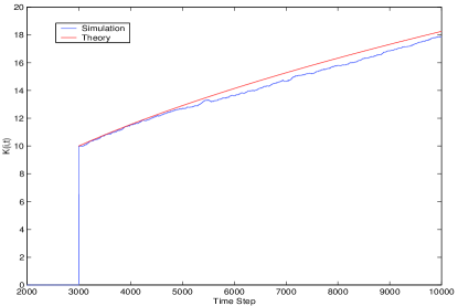
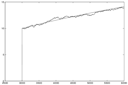
Figure 2: The evolution of the degree of a node inserted in the network. The power-law growth, and its independence from the deletion rate, is at the heart of the results of Section II. The top figure is the plot for the case of 20% deletion rate. The bottom figure is for the case of 70% deletion rate. A node is inserted at time step $t=3000$, and its degree is recorded at future time steps (for $m=10$) until it gets deleted. Over 100 trials, the degree of this node (for the trials where it was not deleted until time step 10000 and 6000, respectively) are averaged and the results are compared to predictions.

Now to calculate the power-law exponent, we note that

$$P(k,t) = \frac{\hbox{No. of nodes with degree $=\ k$}}{\hbox{Total number of nodes}}$$ (9)

$$= \frac{1}{N(t)}\sum_{i:k(i,t)=k}D(i,t)$$

$$= \displaystyle\frac{1}{N(t)}D(i,t)\left|\frac{\partial k(i,t)}{\partial i}\right|_{i:k(i,t)=k}^{-1}$$

From Eqn. (8), we obtain:

$$\frac{t}{i_{k}} = m^{-1/\beta}k^{1/\beta}\ ,$$

and thus,

$$\displaystyle\frac{\partial i}{\partial k}|_{i=i_{k}} = m^{1/\beta}k^{-1/\beta-1}(-1/\beta)t\ .$$ (10)

Inserting it in Eqn. (9), we get

$$P(k,t) = \frac{k^{-\frac{c}{(1-c)\beta}}}{(1-c)m^{\frac{-1}{\beta(1-c)}}}k^{-1/\beta-1}$$ (11)

$$= \frac{k^{-1-\frac{1}{(1-c)\beta}}}{(1-c)m^{\frac{-1}{\beta(1-c)}}}\ ,$$

which is a power-law distribution with the exponent

$$\gamma=-1-\frac{1}{(1-c)\beta}$$ (12)

This equation for obtaining the power-law exponent from Eqn. (8) for a general $\beta$ will be used later on too. For our case of $\beta=1/2$ we get the exponent of

$$|\gamma|=1+\frac{2}{1-c}\ .$$ (13)

As illustrated in Fig. 3, simulation results provide a verification of Eqn. (13).

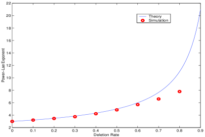
Figure 3: The power-law exponent for the degree distribution of networks generated with the model discussed in Section II. The exponents are the slopes of the best fit line to the log-log plots of the corresponding cumulative distributions. The time steps at which snapshots are taken vary from 20000 to 100000 based on the deletion rate, so that at the time of snapshot, almost 20000 nodes are in the network for all cases. The theory and the simulation results are in perfect agreement for small values of $c$. For larger values of $c$ however, tracking the very fast growing exponent is rather hard. The deviation then seems to be the result of the finite number of time steps. In any case, the value of the exponent for $c>50\%$ is too large for the network to display any of the desirable properties usually associated with scale-free networks.

II.2 Additional preferentially targeted links will not help

We now show that introducing new preferential attachments, as introduced in BB , will not help control the divergence of the exponent. To see this, let us modify the protocol as follows: At each time step, a new node is added and it makes $m$ preferential attachments; $c$ randomly chosen links are deleted; and a randomly chosen node initiates $b$ preferentially targeted links.

Following the same steps, as in the previous section, one can show that $\displaystyle S(t)=\frac{2m(1+c)(b+1)t}{1-c},$ and one can verify that the rate equation would simplify to $\displaystyle\frac{\partial k(i,t)}{\partial t}=m\frac{(1+c)(b+1)k(i,t)}{2m(b+1)(1-c)t}-\frac{c}{1-c}\frac{k(i,t)}{t},$ which is equivalent to Eqn. (8), and results in the same power-law exponent as in Eqn. (13).

II.3 The expected degree of any particular node

The degree of an existing node is governed by Eqn. (8) until it gets deleted, when its degree can be assumed to be $0$. Thus, the expected degree of the $i^{\hbox{th}}$ node at time $t$ is given by (see Dog1 )

$$E(i,t)=K(i,t)D(i,t)$$

$$\displaystyle=m\left(\frac{t}{i}\right)^{-\frac{c}{1-c}+\beta}$$

$$\displaystyle=m\left(\frac{t}{i}\right)^{\frac{-(\beta+1)c+\beta}{1-c}}\ .$$ (14)

Hence, if we define $\displaystyle c_{0}=\frac{\beta}{\beta+1}$, then for $c>c_{0}$, $E(i,t)\rightarrow\infty$, and for $c<c_{0}$, $E(i,t)\rightarrow 0$ when $\displaystyle\frac{t}{i}\rightarrow\infty$.

For our case of $\beta=1/2$, $c_{0}=1/3$. Hence, for high enough deletion rates, a node is not expected to acquire infinite links before it is deleted. Fig. 4 shows simulation results for the average degree of nodes and the change in the behavior of $E(i,t)$ around $c=0.33$ is again in perfect match with our predictions.

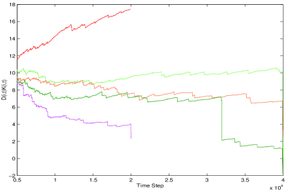
Figure 4: A node is inserted at time step=3000, and its degree is recorded at future time steps. After it is deleted, the degree would be zero for the rest of the time. This quantity is averaged over 100 trials of the process to find $E(i,t)$ defined in (Eqn. II.3). If $c>1/3$, then $E(i,t)$ should go to zero as $i/t\rightarrow\infty$, otherwise it should go to infinity. The curves from top correspond to $c=20\%,30\%,35\%,40\%,50\%$, respectively.

III The Compensation process

We now introduce a local and universal random protocol that will lead to the emergence of true scale-free networks when nodes are deleted at a fixed rate.

III.1 Deletion-Compensation Protocol

Consider the following process, where at each time step:

1. A new node is inserted and it makes $m$ connections to $m$ preferentially chosen nodes.

2. With probability $c$, a uniformly chosen node and all its links are deleted.

3. If a node looses a link, then to compensate for the lost link it initiates $n<n_{\hbox{\small crit}}(c)$ ($n$ is real) links, the targets of which are chosen preferentially. The upper-bound, $n_{\hbox{\small crit}}(c)$, is specified later.

This protocol is simple in its description as well as in implementation. It is also truly local, i.e., the decisions for all nodes (whether to be deleted or to initiate a compensatory link) are independent and based on the node’s own state.

III.2 Properties of the emergent network

III.2.1 Degree distribution

The rate equation formulation for the degree of the $i^{th}$ node at time $t$ can be stated as:

$$\frac{\partial k(i,t)}{\partial t}=m\frac{k(i,t)}{S(t)}-c\frac{k(i,t)}{N(t)}+nc\frac{k(i,t)}{N(t)}+nc\left\langle k(t)\right\rangle\frac{k(i,t)}{S(t)}\ ,$$ (15)

where (I) $S(t)$ is the sum of the degrees of all the nodes in the network at time $t$ (as defined in Eqn. (2)). (II) The first two terms on the right-hand-side are as described in Eqn. (1). (III) The third term accounts for the fact that the $i^{th}$ node initiates $n$ links if it looses one. (IV) The fourth term (where $\left\langle k(t)\right\rangle$ is the average degree of a node) represents the preferential links made to the $i^{th}$ node by other nodes that lost links because of the deletion of a uniformly chosen node. The average degree of a node $\left\langle k(t)\right\rangle=\frac{S(t)}{N(t)}$.

Note that $D(i,t)$ is still given by Eqn. (3). Next, instead of following the approach in Section II for computing $S(t)$ by manipulating the rate equation, we provide a direct method. Let ${\cal E}(t)=S(t)/2$ be the total number of edges/links in the network at time $t$. Then, a simple rate equation for ${\cal E}(t)$ is:

$$\frac{\partial{\cal E}(t)}{\partial t}=m-(c-nc)\left\langle k(t)\right\rangle=m-(c-nc)\frac{S(t)}{N(t)}\ ,$$ (16)

where the first term is the number of edges brought in by an incoming node, and the second term is the net number of edges lost due to random deletion of a node. Substituting $S(t)=2{\cal E}(t)$ and $N(t)=(1-c)t$, we get

$$S(t)=\frac{2m(1-c)}{1+c-2nc}t\;\,\mbox{ and}\;\left\langle k(t)\right\rangle=\frac{2m}{1+c-2nc}=\left\langle k\right\rangle_{c}.$$ (17)

The validity of Eqn. (17) is checked for different values of deletion rates, and the results are reported in Fig. 5.

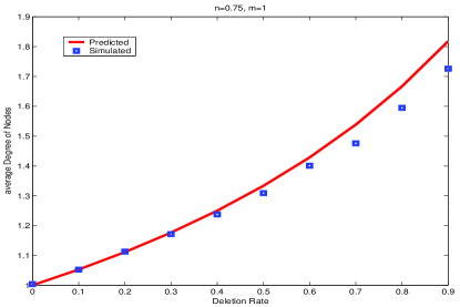
Figure 5: Eqn. (17), states that: $\left\langle k\right\rangle_{c}=\frac{m}{1+c-2cn}$. For the case $n=0.75$, the value $\left\langle k\right\rangle_{c}$ is compared with the simulated results for $0\leq c\leq 0.9$ and $m=1$. The simulations are in good agreement with the predictions, especially for values of $c$ less than $0.7$.

Inserting $S(t)$ back into Eqn. (15) we get:

$$\frac{\partial k(i,t)}{\partial t} = \frac{k(i,t)}{2(1-c)t}(1+c-2nc-2c+4nc)$$ (18)

$$= \frac{k(i,t)}{2(1-c)t}(1-c+2nc)\ .$$

Hence, $\displaystyle k(i,t)=m\left(\frac{t}{i}\right)^{\beta}$, where $\displaystyle\beta=\frac{1-c+2nc}{2(1-c)}$. Next, applying Eqn. (12), we get the power-law exponent to be:

$$\gamma=-1-\frac{2}{1-c+2nc}\ .$$ (19)

Note that, in this case, there is no singularity when $c\rightarrow 1$. In fact for $c=1$ and $0<n\leq n_{\hbox{\small crit}}(1)=1$, we get

$$|\gamma|=1+\frac{1}{n}\ .$$ (20)

The magnitudes of the power-law exponents (calculated as the best fit to the cumulative distribution of the node degrees in simulations) is computed for the range $c=0\%-90\%$, and the results are checked against predictions in Fig.(6).

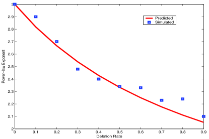
Figure 6: The power-law exponent for different values of the deletion rate. For all values of $c$, the number of nodes at times the snapshots were taken, were kept to be at least 20000. The value of the power-law exponent is the best fit to the histogram of the cumulative data. No fit had regression confidence less than 98.3% for the log-log case . The theoretical curve is depicted in solid. The simulation results are indicated by $\square$.

Note that Eqn. (17) is valid only when the denominator is positive which is equivalent to a finite average degree. So, $1+c-2nc>0$, which implies that $-c+2nc<1$ and $|\gamma|>1+2/(1+1)=2$. This also implies that for any given $c$, $\displaystyle 0<n<n_{\hbox{\small crit}}=\frac{1+c}{2c}$. Thus, for any given deletion rate, $c$, by varying the average number of compensatory edges for each deleted edge, $n$, one can program the magnitude of the power-law exponent, $|\gamma|$, to be anywhere in $(2,\infty)$. Of course, the price one pays for getting close to $-2$, is the associated increase in the average degree, as implied by Eqn. (17). This also, provides a hint for designing network protocols, that is, too many compensatory links might make the network unstable.

III.2.2 The expected degree of a random node at time $t$

Let’s look at the quantity, $E(i,t)$, as defined in Eqn. (II.3):

$$\displaystyle E(i,t) = D(i,t)K(i,t)=m\left(\frac{t}{i}\right)^{-\frac{c}{1-c}+\beta}$$ (21)

$$= m\left(\frac{t}{i}\right)^{\frac{-2c+(1-c+2nc)}{2}{1-c}}$$

$$= m\left(\frac{t}{i}\right)^{\frac{1-c(3-2n)}{2(1-c)}}\ .$$

Thus, for $n=1$ the expected degree becomes independent of $c$, and for and $n>1$ $E(i,t)$ diverges with $t$. Otherwise, for any $n<1$, if $1\geq c>\frac{1}{3-2n}$, then $E(i,t)\rightarrow 0$ as $\frac{t}{i}\rightarrow\infty$. For example, for $n=3/4$ and $c>2/3$, the expected degree of a node will decrease with time. As is well known in the static case, the interesting properties of scale-free networks are due to the divergence of the second moment while having a finite mean, which happens for $|\gamma|<3$. Hence, an interesting quantity would be:

$$E_{2}(i,t) = D(i,t)K^{2}(i,t)$$ (22)

$$= m\left(\frac{t}{i}\right)^{\frac{1-2c(1-n)}{(1-c)}}\ .$$

So, for any $n>0.5$, and irrespective of the value of $c$, $E_{2}(i,t)$ diverges, which is consistent with the fact that for any $n>0.5$, $|\gamma|<3$ and the underlying degree distribution has unbounded variance. Thus, one might want to work in the regime, $1>n>0.5$ and $1\geq c>\frac{1}{3-2n}$, where $E(i,t)\rightarrow 0$ but $E_{2}(i,t)\rightarrow\infty$ as $\frac{t}{i}\rightarrow\infty$. For example, if $n=0.75$ and $c\rightarrow 1$, then one can get an exponent of $-2.33$, and yet have the expected degree of any node to be bounded.

IV Concluding remarks

We first point out a conceptual link between our compensatory rewiring scheme discussed in Section III, and the doubly preferential attachment scheme, as introduced in Dog3 ; chung . By doubly preferential attachment, we mean that for an edge inserted in the network, both the initiator and the target nodes are chosen preferentially based on their degrees. For example, consider the following random protocol: At each time step, a new node is inserted that makes $m$ connections to $m$ preferentially chosen nodes. From the nodes in the network, $l$ nodes are chosen with probability proportional to their degrees. Each of these selected nodes initiates $m$ new links to $m$ preferentially chosen targets. It can be shown Dog3 ; chung that the power-law exponent $\displaystyle|\gamma|=2+\frac{1}{1+2l}$, and hence, by choosing $l$ one can make the exponent as close to $-2$ as desired. In this regard, our compensatory rewiring scheme can be considered as a natural means for introducing doubly preferential attachments. By uniformly deleting nodes, a node looses links with probability proportional to its degree. So a node initiating a compensatory preferential attachment, intrinsically introduces doubly preferential attachments. The random deletions of nodes is thus being used in our stochastic protocol to lead to the emergence of truly scale-free networks.

One of our main motivations for this work was to design random protocols that will solve the problem of organizing a highly-dynamic content sharing network. The first step in this direction would be to design a local and easily implementable protocol that would lead to the emergence of a pre-specified network structure under the usage constraints imposed by the users. As mentioned in the introduction, although the network size usually grows for such networks (more people join such networks), the time scale within which the size changes is much larger than the time scale within which the old members of the network log-in and log-off. Hence, the desired form of the network structure should emerge almost solely due to the dynamics of the protocol and cannot rely too much on the growth rate itself. As regarding the desired structure of the network, motivated by many advantageous aspects of scale free networks, one might want to come up with protocols that could make the network self organize into a scale-free structure with a desired power-law exponent (usually around $-2.5$).

There has been some concern that searches on such power-law networks might not be scalable; however, our recent results show that by using bond percolation on the underlying networks, one can make such networks very efficiently searchable. In particular, we show that for networks having a power-law degree distribution with exponent close to $-2$, a traffic efficient search strategy can be locally implemented. Specifically, we show that $O(\sqrt{N}log^{2}(N))$ communications on those networks are sufficient to find each content with probability $1$. This is to be compared to $\Theta(Nlog(N))$ communications for currently used broadcast protocols. Also, the search takes only $O(log(N))$ time steps scalable . Thus, scale-free structures with exponents close to $-2$, are not only observed in current P2P systems, but also are the desirable structures for realizing a truly distributed and unstructured P2P data-base system.

The very high rate of log-offs in real P2P networks prevents the ordinary preferential attachment scheme from forming a scale free network, with exponents less than $3$ (as shown in the Sec. II). The local compensation process introduced in Sec. III, however, imposes a scale free structure with an exponent that can always be kept below $3$. All a node has to do is to start a new preferential connection, whenever it looses one! Note that this compensatory procedure is quite natural (and probably essential) for networks in which the members have to be part of the giant connected component to be able to have access to almost all other nodes. In fact, in many clients of the existing P2P networks, this condition is imposed by always keeping a constant number of links to active IP addresses. Our numerical simulations show that graphs resulting from our compensatory protocol are almost totally connected; that is, a randomly chosen node with probability one belongs to the giant connected component of the graph even in the limit of $c=1$. Thus, using our decentralized compensatory rewiring protocol one can launch, tune, and maintain a dynamic and searchable P2P content-sharing system.

We also believe that our model can, at least intuitively, account for the degree distributions found in some crawls of P2P networks like Gnutella. As an example, in GNUT , the degree distribution of the nodes in a crawl of the network was found to be a power-law with an exponent of $-2.3$. Although Gnutella protocol Gnut-prot does not impose an explicit standard on how an agent should act when it loses a connection, there are certain software implementations of Gnutella which try to always maintain a minimum number of connections by trying to make new ones when one is lost. Thus, while all clients might not be compensating for lost edges, it is reasonable to assume that at least a certain fraction are. As shown in Sec. III, if we pick $n=0.75$ (i.e. 75% of the lost links are compensated for), and as $c\rightarrow 1$, the degree distribution is indeed a power-law with exponent $-2.33$.

To summarize, we have designed truly local and yet universal protocols which when followed by all nodes result in robust, totally-connected and scale-free networks with exponents arbitrarily close to $-2$ even in an ad hoc, rapidly changing and unreliable environment.

References

- (1) Dorogovtsev, S.N. , Mendes,J.F.F. “Scaling Properties of Scale-free Evolving Networks:Continuous Approach”, Phys. Rev. E 63, 056125 1-19 (2001)
- (2) Bianconi,G, A.L. Barabasi, “Topology of evolving networks: local events and universality”, Phys. Rev. Lett. 85, 5234-5237 (2000)
- (3) Dorogovtsev, S.N. , Mendes,J.F.F., “Scaling Behaviour of Developing and Decaying Networks”,EuroPhys. Lett. 52, 33 (2000)
- (4) P. L. Krapivsky, G. J. Rodgers, S. RednerDegree, “Degree Distributions of Growing Networks,” Phys. Rev. Lett. 86, 5401-5404 (2001)
- (5) Albert,R, A.L.Barabasi “Statistical Mechanics of Complex Networks,”Reviews of Modern Physics 74, 47 (2002)
- (6) William Aiello, Fan Chung, Linyuan Lu, “Random evolution in massive graphs,” IEEE Symposium on Foundations of Computer Science(2001).
- (7) “Clip2 - Gnutella: To the Bandwidth Barrier and Beyond,” www.clip2.com/gnutella.html
- (8) ”The Gnutella Protocol Specification”. Online: http://dss.clip2.com/GnutellaProtocol04.pdf. 2001.
- (9) N. Sarshar, P. O. Boykin, and V. Roychowdhury, “Scalable Parallel Search in Random Power-Law Networks,” in preparation.