Long surface wave instability in dense granular flows.

Abstract

In this paper we present an experimental study of the long surface wave instability that can develop when a granular material flows down a rough inclined plane. The threshold and the dispersion relation of the instability are precisely measured by imposing a controlled perturbation at the entrance of the flow and measuring its evolution along the slope. The results are compared with the prediction of a linear stability analysis conducted in the framework of the depth-averaged or Saint-Venant equations. We show that when the friction law proposed in Pouliquen (1999a) is introduced in the Saint-Venant equations, the theory is able to predict quantitatively the stability threshold and the phase velocity of the waves but fails in predicting the observed cutoff frequency. The instability is shown to be of the same nature as the long wave instability observed in classical fluids but with characteristics that can dramatically differ due to the specificity of the granular rheology.

1 Introduction

Natural gravity flows such as mud flows or debris flows can be destructive. Very often the material does not flow continuously along the slope of mountains, but develops in a succession of surges. These surges are of large amplitude and can be destructive as they are able to carry large debris. The breaking of an initially continuous flow to a succession of waves is often attributed to an inertial instability that can develop in thin liquid flows down slopes. However, while this instability has been extensively studied for the case of Newtonian fluids, the formation of long surface waves in particulate flows has been much less investigated. The goal of this paper is to clarify the dynamics of the long-wave instability for a cohesionless granular material flowing down a rough inclined plane.

Long-wave free surface instability in gravity flows is a phenomenon common to many fluids. For a viscous fluid in the laminar regime, the instability is often called “Kapitza instability” after the pioneering work by Kapitza $\&$ Kapitza (1949). They have observed that a thin film of water flowing along a vertical wall does not remain uniform but deforms in a succession of transverse waves propagating down the wall. Since Kaptiza’s work, many experimental and theoretical studies have been devoted to thin viscous flows down inclined planes (see, for instance, the review of [Chang 1994] or [Oron et al. 1997]). Free surface waves are also observed in turbulent flows down slopes, where they evolve into a series of bores more or less periodic called “roll waves” ([Cornish 1934]; [Dressler 1949]; [Needham & Merkin 1984]; [Kranenburg 1992]). These roll waves are of great importance in hydraulic for flows in open channels. Similar surges are also observed in flows using more complex fluids, e.g. mud flows, gravity currents, flows of particles suspension (see [Simpson 1997]). However, few precise experimental studies can be found for these non Newtonian fluids.

The spontaneous formation of free surface waves in fluids having very different rheological properties comes from the fact that the instability mechanism does not depend on the precise fluid characteristics (see the clear discussion by Smith (1990) in the context of viscous film flows). When a fluid layer flows down an inclined plane, a small perturbation of the free surface propagates at first order with a phase velocity which is different than the mean fluid velocity. If the fluid could adjust instantaneously its velocity to the local thickness variation, the wave would propagate without amplification (kinematic waves, [Witham 1974]). However, because of inertia, the fluid does not immediately adjust its velocity when the wave arrives. This delay can give rise to a positive mass flux under the wave leading to the growth of the perturbation.

From a theoretical point of view, many studies concern the case of laminar Newtonian flows. In this case the linear stability analysis of a film flow can be derived based on the Orr-Sommerfeld equation ([Benjamin 1957]; [Yih 1963]). Amplitude equations and precise non linear models have been also recently developed ([Chang 1994]; [Ruyer-Quil & Manneville 2000]). For non Newtonian complex fluids, exact three dimensional analysis are often not possible because of the lack of sufficient knowledge of the constitutive equations. For those systems, a classical approach for studying the stability of thin flows is the shallow water description. Mass and momentum balances are written in a depth averaged form (Saint-Venant equations, [Saint-Venant 1871]). In this framework, the rheological characteristics of the fluid are mainly taken into account into the expression of the shear stress between the flowing layer and the surface of the plane. The shear stress is a viscous force for laminar Newtonian flows ([Shkadov 1967]), a turbulent friction given by a Chezy formula for turbulent flows ([Kranenburg 1992]), a Bingham stress for mud flows ([Liu & Mei 1994]). It is then possible to study the linear stability analysis of the flow and to predict the threshold and growth of the waves.

Although the free surface instability mechanism is the same for different fluids, the precise characteristics of the wave development (threshold, growth rate,..) dramatically depend on the rheological properties of the material. A precise experimental study of the instability could then serve as a test for the rheological laws proposed for complex fluids. This is the spirit of this paper on the wave formation in cohesionless granular materials. Formation of long waves in granular flows down inclined planes has been reported in previous studies ([Savage 1979]; [Davies 1990], [Vallance 1994]; [Ancey 1997]; [Daerr 2001]). However, to our knowledge no precise measurements of the instability properties have been carried out.

The rheology of dry granular materials flowing in a dense regime is still an open problem ([Rajchenbach 2000]; [Pouliquen & Chevoir 2002]). However, for the flow of thin granular layers on inclined planes, a Saint-Venant description seems to be relevant. Savage and Hutter first proposed this approach for describing the motion of a granular mass down an inclined plane ([Savage & Hutter 1989]). For the basal friction stress they used a solid friction law where the shear stress at the interface between the flowing material and the inclined plane is proportional to the normal stress, i.e. to the weight of the material column above the base. Although this description is able to correctly predict the spreading of a mass on steep slopes and smooth surfaces ([Savage & Hutter 1989]; [Naaim et al. 1997]; [Gray et al. 1999]; [Wieland et al. 1999]), it does not capture the existence of steady uniform flows when the surface is rough and the material sheared in the bulk. Recently, a generalization of the basal friction law has been proposed based on scaling properties observed in experiments ([Pouliquen $1999a$]). The generalization gives a friction coefficient which is no longer constant but depends on the local velocity and thickness. Using this law in Saint-Venant description it is possible to quantitatively predict the motion of a mass down a rough inclined plane from initiation to deposit ([Pouliquen & Forterre 2002]). In this paper we want to check to what extent the same approach using the generalized friction law can quantitatively predict the long wave instability for dry granular materials.

To this end we have carried out precise measurement of the linear development of the instability in the same spirit as Liu et al. (1993) did for liquid films. Liu et al. have developed a method to induce at the entrance of the liquid flow a perturbation whose amplitude and frequency can be controlled. The instability being convective, the observed waves downstream result from the amplification of the entrance perturbations. By following the evolution of the injected perturbation for different frequencies, Liu et al. were able to experimentally measure the dispersion relation and precisely determine the instability threshold. In this paper we follow the same procedure for granular flows: in the limited range of inclinations where steady uniform flows are observed, we impose an external forcing to control the wave development.

The paper is organized as follows. We first present preliminary experimental observations of the instability without forcing ($\S\,2$). We show that a simple visual analysis of the free surface instability is not sufficient to conclude about the instability mechanism and that more precise measurements are necessary. The experimental set up, the forcing method and the measurement procedure are described in $\S\,3$. The linear stability analysis based on Saint-Venant equations is presented in $\S\,4$. Results and comparison between experiments and theory are presented for glass beads in $\S\,5$ and for sand in $\S\,6$. Discussion and conclusion are given in $\S\,7$.

2 Preliminary observations

Free surface waves in granular flows down a rough inclined plane have been reported previously by several authors. Using glass beads, Savage (1979) and Vallance (1994) observed the deformation of the free surface in a succession of surges down a long chute flow. Ancey (1997) reported formation of surge waves with sand. Recently, Daerr (2001) has noticed an instability at the rear of avalanche fronts for flows of glass beads on velvet. All these experiments were performed on rough surfaces in a dense regime, i.e. with a mean volume fraction of the medium almost constant. Waves have also been recently observed for granular flows on flat smooth surfaces ([Prasad et al. 2000]; [Louge & Keast 2001]) but dramatic variations of density are observed in this case, with very dilute regions. We will not discuss this case here.

Figure 1 shows the typical free surface we observe for a flow of sand 0.8 mm in diameter down an inclined plane made rough by gluing one layer of sand grains on it. A silo at the top of the plane (2 m long, 70 cm wide) continuously supplies the flow at a constant flow rate. Waves first appear close to the outlet of the silo as two-dimensional deformations. They rapidly amplify downstream and break down in the transverse direction due to secondary instabilities. The shape of the saturated waves is highly non linear as shown by the typical thickness profile plotted in inset of figure 1. The distance between two surges is typically of the order of 20 cm, which is very large compared to the thickness of the layer (which is about 5 mm for the case of figure 1).

The observed pattern does look similar to patterns observed in liquid flows. However, a major difference appears when changing the experimental conditions, i.e. the thickness of the layer and the inclination of the plane. Figure 2 shows a qualitative phase diagram obtained simply by visual observations of the free surface. The striking result of this preliminary analysis with sand is that the waves are observed mainly close to the threshold of the flow (low inclinations and thin flows). In this region, large amplitude waves are observed. When one increases the thickness of the layer at a fixed inclination, the waves form further and further downstream and eventually disappear for thick flows i.e. for more rapid flows. Naively, one would say that this observation is in contradiction with the explanation in terms of an inertial instability, which should develop preferentially in rapid flows rather than in slow flows.

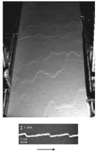
Figure 1: Free surface of the sand flow showing the long surface waves. Material is flowing downwards; the plane width is 70 cm. Inset: typical thickness profile of the natural waves measured with a laser sheet light (see [Pouliquen $1999a$] for the description of the method). The arrow gives the flow direction. (sand 0.8 mm in diameter, $\theta=34^{\circ}$, $h=$4.6 mm).

Another striking preliminary observation is made using glass beads as a granular material. In this case, no wave was observed in our set-up, whatever the thickness and the inclination. The absence of noticeable deformation of the free surface is what made systematic measurements of the steady uniform regime possible and allowed to put in evidence flow scaling laws ([Pouliquen $1999a$]). This point is also intriguing as one would expect the long-wave instability to occur as in other fluids for fast enough flows ([Vardoulakis 2002]).

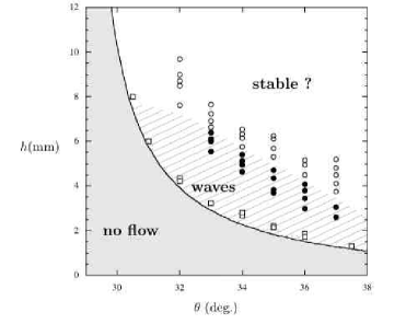
Figure 2: Qualitative stability diagram for sand 0.8 mm in diameter. The hatched zone is the domain where waves are observed. ($\bullet$): waves, ($\circ$): no wave, ($\Box$): flow threshold.

The situation is then rather confused and the preliminary observations raise several questions. First, why are the flow of sand and the flow of glass beads so different? Secondly, in sand the waves seem to develop for slow flows and disappear for rapid flow in apparent contradiction with an inertial instability. Are the waves due to a different instability mechanism? Finally, why is no wave observed with glass beads whereas for rapid flows one would expect the instability to develop? In order to properly answer those questions one need to precisely study the stability of the flow not only by visual observation of the free surface deformation but by careful measurement of the amplification of an initially imposed perturbation. This is the reason why, following Liu and Gollub’s procedure (Liu et al. 1993), we have developed a forcing method.

3 Experimental setup

The experimental set-up is presented in figure 3. The plane is 2 m long and 35 cm wide. The bottom plate as well as the side walls are glass plates. The roughness is made by gluing on the bottom plate one layer of the particle used for the flow. The flow rate is controlled by the opening of the silo. In this paper we have used two granular materials: glass beads $d=0.5$ mm in mean diameter (the same as used in [Pouliquen $1999a$]), and sand $d=0.8$ mm in mean diameter (figure 4).

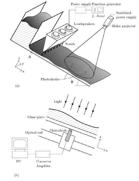
Figure 3: (a) Sketch of the experimental set-up used to force the instability. (b) Description of the light detection method.

3.1 Forcing method

In order to impose a perturbation whose frequency and amplitude can be easily controlled we periodically blow a thin air jet on the free surface. The jet is created by three loudspeakers embedded into a two dimensional nozzle with a 1 mm slit (figure 3$a$). A homogeneous and localized air jet is then created, with an amplitude and a frequency controlled by the amplitude $A_{GBF}$ and frequency $f$ sent to the loudspeakers via a low frequency function generator. The nozzle is placed 30 cm from the outlet of the reservoir. The typical free surface deformation we achieved with this set up is of the order of 0.25 mm and frequency varies between 1 Hz and 20 Hz. A typical response of the free surface to the forcing air jet is plotted in figure 5($a$). In this figure, the measurement is carried out just below the nozzle and the signal sent to the loudspeaker is sinusoidal at a frequency of 3 Hz. One observes that the thickness variation follows the forcing frequency but that the response is not sinusoidal but highly asymmetric. When air is blown, the air jet is localized and the induced deformation important. When the nozzle sucks the air, there is no influence on the free surface. This difference between localized ejection and diffuse injection is well-known and is used, for instance, for propulsion in water. The non sinusoidal response clearly appears on the Fourier transform of the signal in figure 5($b$). The perturbation is periodic at the imposed frequency, but many harmonics are also present with amplitude that can be higher than the fundamental. This effect is more pronounced when the forcing frequency is low. With this forcing method it is then difficult to inject low frequency modes at measurable amplitude, without injecting very high harmonics, which will interact in a non linear regime. Consequently, no measurement of the linear evolution was possible below 1 Hz.

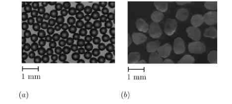
Figure 4: Granular materials used. ($a$) Glass beads $d=0.5\pm 0.05$ mm in mean diameter (grinding glass beads supplied by Potters-Ballotini, France). ($b$) Sand $d=0.8\pm 0.1$ mm in diameter (sand of the Loire supplied by Sifraco, France).

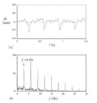
Figure 5: Free surface deformations of the flow below the nozzle ($f=$3 Hz, $A_{GBF}=1.5$ V). ($a$) Thickness variations. ($b$) Fourier transform of the thickness variations, $|a_{f}|$, averaged over 60 cycles (arbitrary units).

3.2 Thickness measurement

In order to measure precisely the free surface deformation we use a light absorption method. A parallel beam lights the plane from above as sketched in figure 3($b$). Two photodetectors are placed at different distances from the nozzle below the plane. The light measured by the detector varies exponentially with the thickness of the granular layer as shown by the calibration curves in figure 6. The light intensity received by the detector is plotted versus the thickness (see [Pouliquen $1999a$] for the thickness measurement method). The data are well fitted by $I=I_{0}\exp(-h/L_{a})$, the attenuation length being larger for the beads $L_{a}$=7.4 $d$, than for the sand $L_{a}$=1.82 $d$. This calibration has been carried out for both uniform layer at rest (black dots) or flowing layers (circles). We observe that the two data sets collapse. Since the light absorption is a function of both the layer thickness and the volume fraction, this collapse means that the variations of the volume fraction are negligible in the dense flow regime studied here.

The signal measured by the photodetector is digitalized by a PC trough an acquisition board at 100 kHz. Notice that from the temporal evolution of the light amplitude, $I(t)$, it is possible without any calibration to get the deformation of the free surface $\delta h(t)=h(t)-\langle h(t)\rangle$ where $\langle h(t)\rangle$ is the mean thickness. The exponential attenuation law leads to the following expression: $\delta h(t)=-L_{a}(\ln I(t)-\langle\ln I(t)\rangle)$, which is independent of $I_{0}$ and of the gain of the photodetectors. With this method the deformation of the free surface is determined with a precision of about 0.05 mm.

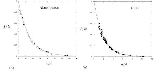
Figure 6: Calibration curve for the light transmitted through a layer of grain as a function of the thickness $h$ of the layer, ($a$) glass beads $d=0.5$ mm in diameter, ($b$) sand $d=0.8$ mm in diameter. ($\bullet$): static layers. ($\circ$): flowing layers. The solid curve is the best exponential fit $I/I_{0}=\exp(-h/L_{a})$ with $L_{a}=7.40\,d$ for glass beads and $L_{a}=1.82\,d$ for sand.

3.3 Measurement of the dispersion relation

From the thickness measurement at two different points it is in principle possible to measure the dispersion relation. To this end a perturbation at a given frequency $f$ is imposed to the flow by our forcing device. The two photodetectors then give the free surface deformations $\delta h(x_{1},t)$ and $\delta h(x_{2},t)$ at two different locations $x_{1}$ and $x_{2}$. By computing the Fourier transform of the deformations, one obtains at the two locations the amplitudes $a_{f}(x_{1})$ and $a_{f}(x_{2})$ and the phases $\phi_{f}(x_{1})$ and $\phi_{f}(x_{2})$ of the fundamental mode at frequency $f$ defined by : $\delta h_{f}(x,t)=a_{f}(x)\cos(2\pi ft-\phi_{f}(x))$. If the evolution between $x_{1}$ and $x_{2}$ is assumed to be exponential, i.e. in the linear regime of the instability, the deformation of the mode $f$ is supposed to vary as: $\delta h_{f}=a_{0}e^{\sigma x}\cos(2\pi f(t-x/v_{\phi}))$. The spatial growth rate $\sigma(f)$ and the phase velocity $v_{\phi}(f)$ are then given by:

$$\sigma(f)=\frac{1}{x_{2}-x_{1}}\ln\left(\frac{a_{f}(x_{2})}{a_{f}(x_{1})}\right),$$ (1)

$$v_{\phi}(f)=\frac{2\pi(x_{2}-x_{1})f}{\phi_{f}(x_{2})-\phi_{f}(x_{1})}.$$ (2)

The dispersion relation can then in principle be determined. Experimentally the difficulty is to determine a region of linear instability where the wave grows exponentially. The amplitude of the deformation has to be small enough to remain in the linear evolution but not too small to be measured.

4 Linear stability analysis

In this section, we present the theoretical analysis of the long-wave instability for granular flows in the framework of the depth-averaged equations. A previous analysis has been carried out by Savage (1989) using a Chezy formula to model the basal shear stress. Here we present the theoretical prediction when the interaction between the granular layer and the rough plane is described by the empirical friction law derived from experimental measurements on steady uniform flows ([Pouliquen $1999a$]).

4.1 Depth-averaged equations

A detailed derivation of depth-averaged equations in the context of granular flows can be found in Savage $\&$ Hutter (1989). Assuming that the flow is incompressible and that the spatial variation of the flow takes place on a large scale compared to the thickness of the flow, we obtain the depth-averaged mass and momentum equations by integrating the full three-dimensional equations. For a two-dimensional flow down a slope making an angle $\theta$ with the horizontal (see figure 7), depth-averaged equations reduce to:

$$\frac{\partial h}{\partial t}+\frac{\partial hu}{\partial x} = 0,$$ (3)

$$\rho\left(\frac{\partial hu}{\partial t}+\alpha\frac{\partial hu^{2}}{\partial x}\right) = \left(\tan\theta-\mu(u,h)-K\frac{\partial h}{\partial x}\right)\rho gh\cos\theta,$$ (4)

where $h$ is the local thickness of the flow and $u$ is the averaged velocity defined by $u=Q/h$, $Q$ being the flow rate per unit of width.

The first equation (3) is the mass conservation. The second equation (4) is the momentum equation where the acceleration is balanced by three forces. In the acceleration term, the coefficient $\alpha$ is related to the assumed velocity profile across the layer and is of order 1. We will discuss the role of the parameter $\alpha$ in $\S\,5$. The first force in the right-hand side is the gravity parallel to the plane. The second term is the tangential stress between the fixed bottom and the flowing layer; it is written as a friction coefficient $\mu$ multiplied by the vertical stress $\rho gh\cos\theta$. The friction coefficient is assumed to depend only on the local thickness $h$ and the local velocity $u$. This is a generalization of Savage $\&$ Hutter (1989)’s assumption of a constant solid friction. However, the friction coefficient $\mu$ could depend on other quantities such as the normal stress or the derivatives of $h$ and $u$. The last term in (4) is a pressure force related to the thickness gradient. The coefficient $K$ represents the ratio of the normal stress in the horizontal direction ($x$-direction) to the normal stress in the vertical direction ($z$-direction). Recent numerical simulations have shown that for dense granular flows the horizontal and the vertical normal stresses are almost equal (Prochnow et al. 2000, Ertas et al. 2001). Therefore, we will take $K=1$ in the following. However, it should be noticed that for non uniform flows, the factor $K$ could depend on the divergence of the flow ([Gray et al. 1999]; [Wieland et al. 1999]).

The great advantage of the Saint-Venant equations is that the dynamics of the flowing layer can be predicted without knowing in details the internal structure of the flow, although some information of the flow dynamics is lost. The complex and unknown three-dimensional rheology of the material is taken into account only in the friction term $\mu(u,h)$. Moreover, this friction is easily determined experimentally by studying steady uniform flows. These flows simply result from the balance between gravity and friction, i.e. $\mu(u,h)=\tan\theta$. This means that measuring how the mean velocity $u$ varies with the thickness $h$ and inclination $\theta$ is sufficient to determine the friction law. Knowing the function $u(h,\theta)$ is then equivalent to knowing the friction law (see [Pouliquen $1999a$]).

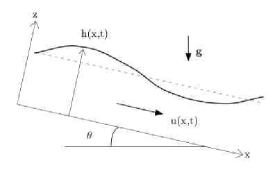
Figure 7: Sketch of the flow.

4.2 Stability analysis

We study here the stability of a steady uniform flow of thickness $h_{0}$ and averaged velocity $u_{0}$. For the sake of simplicity, we first re-write the Saint-Venant equations (3) and (4) with the dimensionless variables given by: $\tilde{h}=h/h_{0}$, $\tilde{u}=u/u_{0}$, $\tilde{x}=x/h_{0}$ and $\tilde{t}=(u_{0}/h_{0})t$. We then obtain:

$$\frac{\partial\tilde{h}}{\partial\tilde{t}}+\frac{\partial\tilde{h}\tilde{u}}{\partial\tilde{x}} = 0,$$ (5)

$${F}^{2}\left(\frac{\partial\tilde{h}\tilde{u}}{\partial\tilde{t}}+\alpha\frac{\partial\tilde{h}{\tilde{u}}^{2}}{\partial\tilde{x}}\right) = \left(\tan\theta-\mu(\tilde{u},\tilde{h})-\frac{\partial\tilde{h}}{\partial\tilde{x}}\right)\tilde{h},$$ (6)

where $F$ is the Froude number defined by:

$$F=\frac{u_{0}}{\sqrt{gh_{0}\,\cos\theta}}.$$ (7)

The two dimensionless control parameters of the problem are therefore the Froude number $F$ and the angle of inclination $\theta$.
We look for steady uniform solutions given by:

$$\tilde{h}(\tilde{x},\tilde{t})=1,\;\tilde{u}(\tilde{x},\tilde{t})=1.$$ (8)

For this basic state, the mass conservation (5) is satisfied and the momentum equation (6) reduces to the balance between gravity and friction: $\mu(1,1)=\tan\theta.$ The next step is to study the stability of (8) by perturbing the flow: $\tilde{h}(\tilde{x},\tilde{t})=1+h_{1}(\tilde{x},\tilde{t})$, $\tilde{u}(\tilde{x},\tilde{t})=1+u_{1}(\tilde{x},\tilde{t})$ with ($h_{1}(\tilde{x},\tilde{t})\ll 1$, $u_{1}(\tilde{x},\tilde{t})\ll 1$) and by linearizing the depth-averaged equations which become:

$$\frac{\partial h_{1}}{\partial\tilde{t}}+\frac{\partial h_{1}}{\partial\tilde{x}}+\frac{\partial u_{1}}{\partial\tilde{x}} = 0,$$ (9)

$${F}^{2}\left(\frac{\partial u_{1}}{\partial\tilde{t}}+(\alpha-1)\frac{\partial h_{1}}{\partial\tilde{x}}+(2\alpha-1)\frac{\partial u_{1}}{\partial\tilde{x}}\right) = -au_{1}-bh_{1}-\frac{\partial h_{1}}{\partial\tilde{x}},$$ (10)

where the dimensionless variables $a$ and $b$ are related to the friction law $\mu(\tilde{u},\tilde{h})$ by:

$$a={\left(\frac{\partial\mu}{\partial\tilde{u}}\right)}_{0},\;b={\left(\frac{\partial\mu}{\partial\tilde{h}}\right)}_{0},$$ (11)

(the index ‘0’ means that the derivatives are calculated for the basic state). Note that to derive (10), we have used the mass conservation (9).

We then seek normal mode solutions for the perturbations: $h_{1}(\tilde{x},\tilde{t})=\hat{h}\exp i(\tilde{k}\tilde{x}-\tilde{\omega}\tilde{t})$ and $u_{1}(\tilde{x},\tilde{t})=\hat{u}\exp i(\tilde{k}\tilde{x}-\tilde{\omega}\tilde{t})$ where $\tilde{k}$ is the dimensionless wavenumber and $\tilde{\omega}$ is the dimensionless pulsation, which, once introduced in the linearized equations (9) and (10), gives the following dispersion relation:

$$-\tilde{\omega}^{2}+2\alpha\tilde{\omega}\tilde{k}+\frac{i}{F^{2}}\left((a-b)\tilde{k}-a\tilde{\omega}\right)+\left(\frac{1}{F^{2}}-\alpha\right)\tilde{k}^{2}=0.$$ (12)

From this dispersion relation, we can easily compute the spatial growth rate and the phase velocity of the waves for a given imposed real pulsation. Computation of the spatial stability analysis is given in Appendix A. This analysis shows that the flow is unstable when:

$$1-\frac{b}{a}>\alpha+\sqrt{\alpha(\alpha-1)+\frac{1}{F^{2}}}.$$ (13)

The above stability criterion is expressed as a function of $a$ and $b$ written in terms of the derivatives of the friction law $\mu(u,h)$. Experimentally, we have access to the relation $u(h,\theta)$ for steady uniform flows. It is therefore useful to write a stability criterion using the relation $u(h,\theta)$ instead of $\mu(u,h)$. Moreover, we will see that this formulation gives an interpretation of the long-wave instability in terms of waves interactions.

As for steady uniform flows we have $\mu(u,h)=\tan(\theta(u,h))$, it is easy to show that:

$$a=\frac{1}{\cos^{2}\theta}{\left(\frac{\partial\theta}{\partial\tilde{u}}\right)}_{0},\mbox{ and}\;\frac{b}{a}=-{\left(\frac{\partial\tilde{u}}{\partial\tilde{h}}\right)}_{0}.$$ (14)

The stability criterion (13) may therefore be written as:

$$\tilde{c}_{0}>\tilde{c}_{+},$$ (15)

where

$$\tilde{c}_{0} = 1+\left(\frac{\partial\tilde{u}}{\partial\tilde{h}}\right)_{0},$$ (16)

$$\tilde{c}_{+} = \alpha+\sqrt{\alpha(\alpha-1)+\frac{1}{F^{2}}}.$$ (17)

It can be shown that $\tilde{c}_{0}$ is the (dimensionless) velocity of the kinematic waves, whereas $\tilde{c}_{+}$ is the (dimensionless) velocity of the “gravity waves” that propagate downstream (see Appendix B). The stability criterion (15) therefore means that the flow is unstable when the velocity of the kinematic waves is larger than the velocity of the gravity waves. Using this formulation, one can then conclude about the stability of the flow just from the velocity law $u(h,\theta)$ of steady uniform flows.

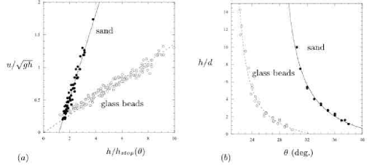
Figure 8: ($a$) Measurements of the averaged velocity of steady uniform flows $u$ as a function of the thickness $h$ and the angle of inclination $\theta$ for glass beads $d=$0.5 mm ($\circ$) ([Pouliquen $1999a$]) and sand $d=$0.8 mm ($\bullet$). The data collapse on a curve when $u/\sqrt{gh}$ is plotted as a function of $h/h_{stop}(\theta)$. ($b$) deposit function $h_{stop}(\theta)$ for the glass beads ($\circ$) and the sand ($\bullet$). The solid line is an interpolation given by $h_{stop}(\theta)=L((\tan\delta_{2}-\tan\delta_{1})/(\tan\theta-\tan\delta_{1})-1)$ where ($L/d=1.65$, $\delta_{1}=20.90^{\circ}$, $\delta_{2}=32.76^{\circ}$) for the glass beads and ($L/d=2.03$, $\delta_{1}=27.0^{\circ}$, $\delta_{2}=43.4^{\circ}$) for the sand.

4.3 Velocity law for granular materials

In this study we use two different granular materials: glass beads and sand. The velocity law for the glass beads has been previously measured ([Pouliquen $1999a$]). The mean velocity $u$, the inclination $\theta$ and the thickness $h$ are related through the following relation:

$$\frac{u}{\sqrt{gh}}=\beta\frac{h}{h_{stop}(\theta)}.$$ (18)

where $\beta=0.136$. The function $h_{stop}(\theta)$ is the thickness of the deposit left by a steady uniform flow at the inclination $\theta$ ([Pouliquen & Renaut 1996]; [Daerr & Douady 1999]).

In order to know the velocity law for the 0.8 mm sand we have also performed the same systematic measurements of the mean velocity as a function of thickness and inclination. We observe that, as for glass beads, the velocity is correlated to the deposit function $h_{stop}(\theta)$ as shown in figure 8. However, the master curve is different for sand and glass beads.

We can therefore write the velocity law in the cases of glass beads and sand in a similar form:

$$\frac{u}{\sqrt{gh}}=-\gamma+\beta\frac{h}{h_{stop}(\theta)},$$ (19)

with

$$\left\{\begin{array}[]{lllllll}\gamma&=&0&\beta&=&0.136&\mbox{for glass beads},\\ \gamma&=&0.77&\beta&=&0.65&\mbox{for sand},\end{array}\right.$$

(the function $h_{stop}(\theta)$ for the glass beads and the sand is given in the caption of figure 8).

From this relation we can then apply the stability criterion (15) which compares the kinematic wave velocity and the gravity wave velocity. To compute the velocities, one needs to know the coefficient $a$ and $b$ given by the (14). From (19), one obtains:

$$a=-\frac{h_{stop}(\theta)}{{\cos}^{3/2}\theta{h_{stop}}^{\prime}(\theta)}\frac{F}{(F\sqrt{\cos\theta}+\gamma)},\mbox{ and}\;\frac{b}{a}=-\left(\frac{3}{2}+\frac{\gamma}{F\sqrt{\cos\theta}}\right).$$ (20)

The (dimensionless) velocity of the kinematic waves given by (16) is therefore:

$$\tilde{c}_{0}=\frac{5}{2}+\frac{\gamma}{F\sqrt{\cos\theta}}.$$ (21)

The speed of the gravity waves depends on the parameter $\alpha$ (see 17). With $\alpha=1$, the instability condition takes a particularly simple expression:

$$F>\frac{2}{3}\left(1-\frac{\gamma}{\sqrt{\cos\theta}}\right).$$ (22)

The linear stability analysis predicts therefore an instability for granular flows when the Froude number is above a critical Froude number $F_{c}$. For glass beads ($\gamma=0$) the critical Froude number is independent of the angle of inclination and given by $F_{c}=2/3$. In the next section, we will compare these theoretical predictions to the experimental studies.

5 Results for glass beads

We first present the experimental results for the flow of glass beads. When there is no forcing, no wave was observed. By imposing a forcing at the entrance of the flow we show that the instability exists but that the spatial growth rates are small. Our inclined plane was therefore too short to allow the observation of the natural instability.

5.1 Spatial evolution of a forcing wave: existence of a linear regime

An example of an amplification of the imposed perturbation is shown in figure 9. The typical temporal signals measured at two locations in the unstable regime ($\theta=29^{\circ}$, $h=$ 5.3 mm) is shown for a forcing frequency $f=$2 Hz. First, we note that the instability is convective, i.e. the periodic perturbation imposed at the entrance is carried downstream by the flow. We also observe that the wave strongly evolves along the plane: in the power spectra figures 9($b$) and 9 ($d$) the fundamental mode and the first harmonic of the forced wave are amplified downstream whereas high-frequency harmonic modes are damped. The amplification of the low-frequency perturbations is also observed on the spectra of the natural noise.

At this stage, an important question is whether the amplification of the low-frequency modes of the forcing waves results from a linear instability or from non linear interactions between modes. Figure 10 shows the spatial evolution of the fundamental mode of a forced wave along the slope for different forcing frequencies (the control parameters are the same as in figure 9). We observe that the forcing modes evolve exponentially along the plane, which implies that we are studying the linear development of the instability.

Another proof of the existence of a linear region is given in figure 11($a$), which shows the spatial growth rate $\sigma$ of a forced mode as a function of its frequency $f$. The black bullets are measurements obtained by imposing a forcing at different frequencies $f$ and measuring the growth rate of the fundamental mode $f$. The other curves are obtained by keeping the forcing frequency $f_{0}$ constant and measuring the growth rate of all the harmonics $f_{0}$, $2f_{0}$, $3f_{0}$…. We observe that both methods give the same curves $\sigma(f)$, which shows that the different harmonic modes of the forced waves weakly interact and evolve quasi-independently in a linear regime.

5.2 Dispersion relation

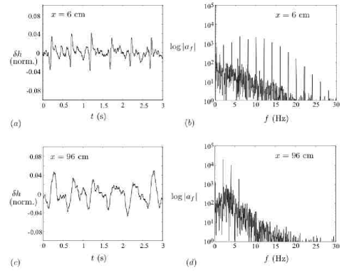
Figure 9: Wave measurement at two distances from the nozzle, $x=6$ cm and $x=96$ cm, in the unstable regime. ($f=2$ Hz, $\theta=29^{\circ}$, $h=$ 5.3 mm). ($a$) and ($c$) Local thickness variations. ($b$) and ($d$) Power spectra averaged on 40 cycles.

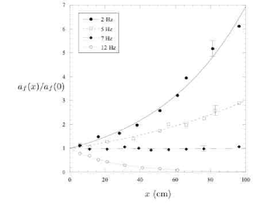
Figure 10: Spatial evolution of the amplitude of the fundamental mode for different forcing frequencies. The distance $x$ is measured from the nozzle. The solid curves are the best exponential fits $\exp(\sigma x)$ with $\sigma(2Hz)=$0.0194 cm^-1, $\sigma(5Hz)=$0.0110 cm^-1, $\sigma(7Hz)=$0.0001 cm^-1 and $\sigma(12Hz)=$-0.0389 cm^-1. The error bars indicate the dispersion of the results. ($\theta=29^{\circ}$, $h=$ 5.3 mm).

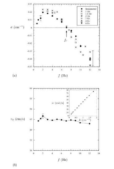
Figure 11: Experimental dispersion relation ($\theta=29^{\circ}$, $h=$ 5.3 mm). ($a$) Spatial growth rate $\sigma$ as a function of the frequency measured from the fundamental mode of the forced wave ($\bullet$) and from the harmonic modes (in that case, the forcing frequency is given in the inset). ($b$) phase velocity as a function of the frequency. Inset: pulsation $\omega$ as a function of the wavenumber $k$.

The existence of a linear region for the instability allows the precise measurement of the linear dispersion relation of the surface waves. To measure the growth rate, the two photodetectors are separated by 60 cm.

A typical experimental dispersion relation is presented in figure 11 for the above control parameters ($\theta=29^{\circ}$, $h=$ 5.3 mm). First, we note in figure 11($a$) that the spatial growth rate of a mode varies with the frequency. For low-frequencies, the spatial growth rate is positive, i.e. the amplitude of the mode is amplified along the plane as shown in figure 10 (2 Hz and 5 Hz). The flow is therefore unstable for the considered control parameters. There exists a cutoff frequency for which the amplitude of the mode remains constant all along the plane (see the mode $f=$7 Hz in figure 10). For higher frequencies, the amplitude decays along the plane and the mode is stable (see the mode $f=$12 Hz in figure 10). We shall see that the existence of a well-defined cutoff frequency $f_{c}$ will allow us to determine precisely the stability threshold. The cutoff frequency $f_{c}$ can typically be determined with a precision of about 0.5 Hz.

The phase velocity of the wave as a function of the frequency can also be determined as shown in figure 11($b$). We observe that the phase velocity $v_{\phi}$ is almost independant of the frequency (the variations of $v_{\phi}$ are within the error bars), which means that the system is non dispersive within the range of frequency explored in the experiment (see also the inset). For $\theta=29^{\circ}$ and $h=$ 5.3 mm, $v_{\phi}\approx$45 cm$/$s, which is a little more than the double of the average velocity of the flow ($u\approx$22 cm$/$s). We have systematically measured the phase velocity for other values of the control parameters ($\theta$,$h$). The phase velocity is always nearly independent of the frequency. However, its value depends on the parameters ($\theta$,$h$) as we shall see in $\S\,5.4$.

5.3 Stability threshold

So far, the results have been presented for a given inclination $\theta$ and thickness of the flow $h$. When decreasing the thickness of the flow at fixed $\theta$, we observe that both the cutoff frequency and the growth rate of the most unstable mode decrease as shown in figure 12. The flow is then less unstable as the thickness of the flow decreases and eventually becomes stable below a critical thickness $h_{c}$.

In order to measure precisely the stability threshold $h_{c}$, we have systematically measured the cutoff frequency $f_{c}$ as a function of the thickness $h$ as shown in figure 13($a$). The neutral stability curve $f_{c}(h)$ is then extrapolated to zero frequency in order to determinate $h_{c}$. In order to get a good estimation of the critical thickness we have chosen to interpolate the stability curve $f_{c}(h)$ with two polynomials (see the caption of figure 13). For $\theta=29^{\circ}$, we obtain $h_{c}(29^{\circ})=2.6\pm$0.3 mm. The same method can be applied to measure the critical Froude number $F_{c}$, where the Froude number, $F=u/\sqrt{gh\cos\theta}$, is measured for each set of ($\theta$,$h$) (see figure 13$b$). In that case, the two control parameters are ($\theta$,$F$) instead of ($\theta$,$h$). For $\theta=29^{\circ}$, we find $F_{c}(29^{\circ})=0.54\pm$0.02.

The entire procedure is applied for different angles of inclination. Results are shown in figure 14 which gives the cutoff frequency of the waves as a function of the Froude number $F$. Note that no measurement was made for $\theta$ above $29^{\circ}$ or $\theta$ below $24^{\circ}$. For $\theta>29^{\circ}$, the flow is no longer in a steady uniform regime but accelerates along the slope and leaves the dense regime. For $\theta<24^{\circ}$, the flow rate required to reach the instability increases dramatically. Even with an amount of granular material as large as 150 liters, the total duration of the flow at the threshold is not long enough to allow precise measurements of the stability threshold. This limitation also explains the large uncertainty at $\theta=24^{\circ}$ and why no measurement has been made for high Froude numbers at this angle.

We observe in figure 14 that the cutoff frequencies obtained at different angles collapse close to the threshold when plotted as a function of the Froude number. This result implies that the instability is controlled by the Froude number, at least near the stability threshold.

From these measurements we can determine the stability diagram of the flow in the phase space ($\theta$,$h$) or ($\theta$,$F$), as presented in figure 15. We note that the instability takes place for high inclinations and high thicknesses. The control parameter is the Froude number as shown in figure 15($b$). While the critical thickness $h_{c}$ strongly varies with the angle of inclination of the plane, the critical Froude number $F_{c}$ weakly depends upon $\theta$. For glass beads, we find $F_{c}=0.57\pm 0.05$.

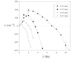
Figure 12: Spatial growth rate as a function of the frequency for different thicknesses of the flow $h$ and a fixed angle $\theta=29^{\circ}$. The corresponding Froude numbers are 1.02 ($\bullet$), 0.66 ($\blacksquare$), 0.58 ($\circ$) et 0.51 ($\Box$).

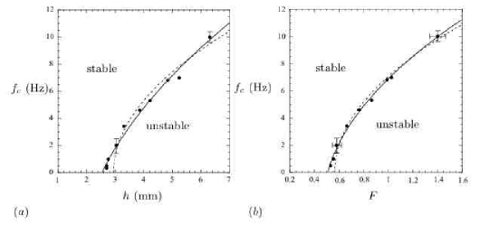
Figure 13: Neutral stability curve for $\theta=29^{\circ}$. The cutoff frequency $f_{c}$ is shown either as a function of the thickness of the flow $h$ ($a$) or as a function of the Froude number $F$ ($b$). The solid curve is a polynomial fit of the type $F,h=a+bf_{c}+cf_{c}^{2}$ and the dashed curve is a quadratic fit of the type $F,h=a+cf_{c}^{2}$.

5.4 Comparison with the theory

The main experimental results of the instability for glass beads are:

• The stability threshold is controlled by the Froude number. Waves appear above a critical Froude number given by $F_{c}=0.57\pm 0.05$.

• The surface wave instability is a long-wave instability, i.e. the first unstable mode is at zero frequency (zero wavenumber). Above the stability threshold, there exists a cutoff frequency for the instability.

• Within the frequency range investigated, the phase velocity of the waves weakly depends upon the frequency, i.e. the media is non dispersive.

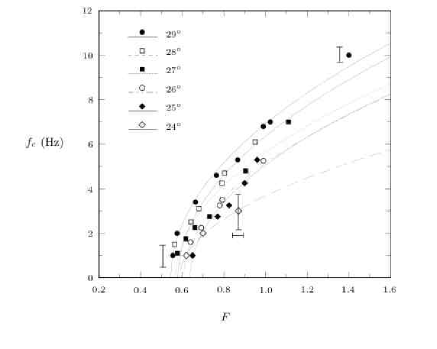
Figure 14: Neutral stability curve $f_{c}(F)$ for different inclination $\theta$. The continuous curves shows for each angle a fit of the type $F=a+bf_{c}^{2}$.

In this section, we compare these results with the prediction of the linear stability analysis performed in the framework of the depth-averaged equations (see § 4). We have seen that this analysis gives the stability threshold and the spatial relation of dispersion as a function of the velocity law $u(h,\theta)$ which, for glass beads, is given by (18).

The only parameter that is unknown in the theory is the parameter $\alpha$ in the acceleration term of the Saint-Venant equations. This parameter is related to the unknown velocity profile across the layer (see §  4.1). For a granular flow down an inclined plane, there is no experimental measurement of the velocity profile but $\alpha$ is close to one. In the following, we will take $\alpha=1$ for the sake of simplicity. We will discuss in more details the influence of $\alpha$ at the end of the section.

5.4.1 Stability threshold

We first compare the theoretical and the experimental stability threshold. For glass beads, we have seen that the linear stability analysis predicts an instability when:

$$F > \frac{2}{3},$$ (23)

$$\mathrm{or}\;\;h > \frac{2}{3}\frac{\sqrt{\cos\theta}}{\beta}h_{stop}(\theta).$$ (24)

The theoretical prediction is given in figure 15 by the dashed curve. We note that the agreement between the experimental data and the theory is relatively good concerning the variation of the critical thickness with the angle and for the order of magnitude of the critical Froude number. However, the theory predicts a critical Froude number that is about $15-20\%$ higher than the experimental one.

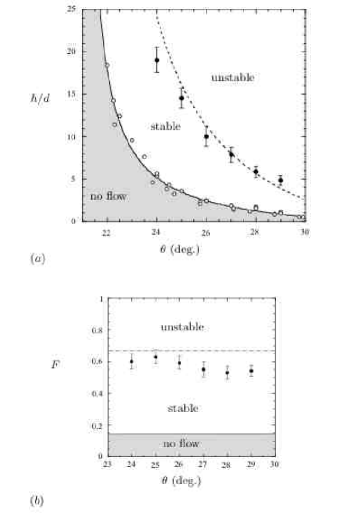
Figure 15: Stability diagram for glass beads in the phase space ($\theta$, $h$) ($a$) and ($\theta$, $F$) ($b$). ($\bullet$): experiments, dashed lines: theoretical predictions. The circles ($\circ$) in ($a$) is the deposit function $h_{stop}$.

5.4.2 Dispersion relation

The linear stability analysis gives also the spatial dispersion relation for the waves. A typical comparison between theory and experiment is given in figure 16, which shows on the same graph the predicted dispersion relation and the experimental data for a given set of control parameters ($\theta=29^{\circ}$, $F=$1.02). We note that the main discrepancy between theory and experiment is that the linear stability analysis does not predict a cutoff frequency for the waves (figure 16$a$). No term in the Saint-Venant equations stabilizes the short wavelengths. However, the linear stability analysis gives the good order of magnitude for the maximum growth rate of the instability, when one compares the maximal growth rate measured in the experiment and the maximal growth rate predicted by the theory.

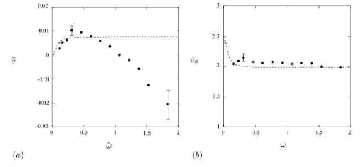
Figure 16: Theoretical (dashed line) and experimental ($\bullet$) dispersion relation for $\theta=29^{\circ}$ and $F=$1.02. ($a$) spatial growth rate $\tilde{\sigma}$ as a function the pulsation $\tilde{\omega}$. ($b$) phase velocity $\tilde{v_{\phi}}$. $\tilde{\sigma}$, $\tilde{v}_{\phi}$ and $\tilde{\omega}$ are nondimensionalized using the thickness of the flow $h=5.3$ mm and the averaged velocity of the flow $u=$21.7 cm$/$s.

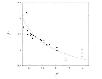
Figure 17: ($\bullet$) experimental phase velocity $\tilde{v}_{\phi}$ as a function of the Froude number $F$ for different angles of inclination $(24^{\circ}-29^{\circ})$. For each ($\theta$, $F$) parameter, $\tilde{v}_{\phi}$ is obtained by averaging the dispersion relation over the frequency. The solid curve is the velocity of the gravity waves $\tilde{c}_{+}=1+(1/F)$ ($\alpha=1$).

It is also interesting to compare the experimental phase velocity to the one predicted by the linear stability analysis (figure 16$b$). We observe that within the frequency range investigated in the experiment, the theory predicts a constant phase velocity, in good agreement with the experimental data. The theory also predicts an increase of the phase velocity for very low frequencies which we are unable to test with our forcing method. It must be noticed that the two limits of the theoretical phase velocity have a precise physical meaning. For $\tilde{\omega}=0$, $\tilde{v}_{\phi}$ is equal to the velocity of the kinematic waves $\tilde{c}_{0}=5/2$ while for $\tilde{\omega}\to\infty$, $\tilde{v}_{\phi}$ tends to the velocity of the gravity waves $\tilde{c}_{+}=1+(1/F)$ (see §  4.3).

We have confirmed this result by systematically measuring the phase velocity of the waves for different angles of inclination and Froude numbers. The data are presented in figure 17. We observe that the experimental phase velocity is always close to the speed of the gravity waves (solid line).

5.4.3 Influence of the parameter $\alpha$ related to the velocity profile

The results of the linear stability analysis presented previously are obtained with the parameter $\alpha$ equal to 1. This parameter appears in the Saint-Venant equations in the acceleration (§ 4.1) and is defined by $\alpha=\langle u^{2}\rangle/{\langle u\rangle}^{2}$. It is therefore necessary to make an assumption on the velocity profile across the layer to know the value of $\alpha$. The value $\alpha=1$, corresponding to a plug flow, was used in the pioneered work of Savage $\&$ Hutter (1989). More recent studies on granular surface flows assume that the velocity profile is linear and use therefore the value $\alpha=4/3$ (Khakar et al. 1997, Douady et al. 1999). For a granular flow down a rough inclined plane, recent numerical simulations suggest that the velocity profile does not remain linear for thick layers but is close to a Bagnold profile ([Ertas et al 2001]), i.e. varies as $z^{3/2}$ ($\alpha=5/4$). From the instability criterion (15), we obtain for $\alpha=5/4$ (resp. $\alpha=4/3$ ) a critical Froude number $F_{c}=0.89$ (resp. $F_{c}=1,03$) to be compared with the experimental value $F_{c}=0.57\pm 0.05$. Paradoxically, the prediction of the theory (for both the threshold and the wave velocity) seems to be better with $\alpha=1$.

These results show that taking into account the velocity profile by a constant parameter $\alpha$ in the depth-averaged equations is not very satisfying. This result is well known in the case of viscous liquid films. It has been shown (see [Ruyer-Quil & Manneville 2000] for instance) that the simple Saint-Venant equations do not predict quantitatively the primary instability if one introduces $\alpha=6/5$ corresponding to the parabolic velocity profile observed in viscous flows. Comparison between the full linear stability analysis of the Navier-Stokes equations and the prediction of the Saint-Venant equations has shown that the latter overestimates the stability threshold by about 20$\%$. This difference between the exact three-dimensional resolution and the averaged equations comes from the fact that for non stationary flows, the shear stress at the base is no longer exactly given by its expression for steady uniform flows ([Ruyer-Quil & Manneville 2000]).

It is therefore doubtful to assign a precise physical meaning to the value of the parameter $\alpha$ in the depth-averaged equations. At best, one may consider $\alpha$ as a “fit parameter” in the equations and the simple value $\alpha=1$ works well in our case.

6 Results for sand

The visual preliminary observations with sand were different than with glass beads. Waves were observed without forcing for slow flows but seemed to disappear for rapid flows in apparent contradiction with an inertial instability. In this section, we show that the forcing method allows to clarify the situation.

6.1 Experimental results

We have measured the dispersion relation of the waves for the sand with the same method used for the glass beads. However, important difficulties arise in the case of sand. Since the flow with sand is strongly unstable, it is difficult to define a linear region where the waves grow exponentially. Moreover, the large noise associated with the natural instability makes the measurements much less reproducible than with glass beads. It is therefore more difficult to quantitatively measure the dispersion relation with the sand than with glass beads. In order to measure the growth rate, we have chosen the following method. First, the two photodiodes are located very close to the nozzle $x_{1}=2$ cm and $x_{2}=10$ cm to prevent as much as possible the non linear evolution of the waves. Then, for each frequencies $f$, the growth rate defined as $\sigma(f)=(1/(x_{2}-x_{1}))\ln(a_{2}/a_{1})$ is averaged over many measurements, carried out at different forcing amplitudes and forcing frequencies.

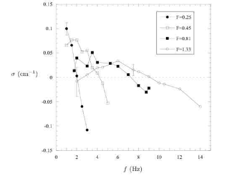
Figure 18: Results for sand 0.8 mm in diameter. Spatial growth rate as a function of frequency for different Froude numbers ($\theta=35^{\circ}$). The corresponding thicknesses of the flow are $h=3.3$ mm ($\bullet$), $h=4$ mm ($\Box$), $h=5$ mm ($\blacksquare$) and $h=6$ mm ($\circ$).

In spite of the uncertainties and the large error bars, the general trend of the dispersion relation can be measured as shown in figure 18, which presents the evolution of the growth rate $\sigma(f)$ with the frequency for different Froude numbers, at a fixed angle $\theta=35^{\circ}$. This plot has to be compared with the one obtained for glass beads (figure 12). We observe that for a given Froude number, the variation of the growth rate with the frequency is similar to the glass beads. The low frequencies are amplified while modes above a given cutoff frequency are damped. However, the order of magnitude of the growth rate for the sand is between $0.02$ cm^-1 and $0.1$ cm^-1, which is about five times the typical growth rate measured with glass beads. This explains why the natural instability is easily observed with sand and not with glass beads.

Another difference between sand and glass beads arises when studying the influence of the Froude number. For sand, the growth rate of the most unstable mode increases as the Froude number decreases by contrast with glass beads. The most unstable mode is observed for $F=0.25$, which corresponds to the slowest flow that may be achieved at this angle. This result is all the more surprising since the cutoff frequency decreases when the Froude number decreases, as observed before with glass beads.

These results are confirmed for other angles of inclination. Figure 19($a$) gives the growth rate of the most unstable mode $\sigma_{max}$ as a function of the Froude number for all the angles studied ($32^{\circ}<\theta<36^{\circ}$). Considering the experimental difficulties, precise measurements are carried out for each angle only for two extreme flows: a slow flow very close to the flow threshold and a fast flow, corresponding to the limits of our set-up. In this figure, we notice that $\sigma_{max}$ is much larger for low Froude flows close to the flow limit (grey zone) than for high Froude flows. On the other hand, $\sigma_{max}$ remains positive even at high Froude number, which means that the flow is still unstable. Therefore, the preliminary observation that the waves disappear at high Froude number comes simply from the fact that the maximum growth rate is a decreasing function of the Froude number.

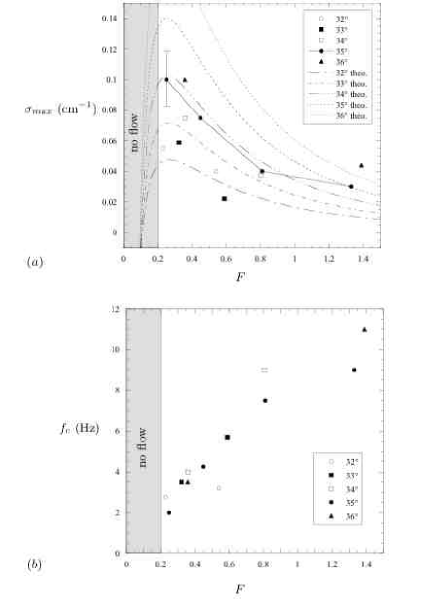
Figure 19: Results for sand 0.8mm in diameter. ($a$) spatial growth rate of the most unstable mode $\sigma_{max}(F)$; ($b$) neutral stability curve $f_{c}(F)$ for different inclination angles (given in the inset). The lines give the theoretical predictions ($\alpha=1$).

It is also interesting to observe the behavior of the cutoff frequency $f_{c}$ with the Froude number (figure 19$b$). We notice that $f_{c}$ decreases when $F$ decreases, which is the signature of a “high-Froude-number-instability”. However, a range of unstable frequencies still exists for the smallest Froude number $F_{min}\approx 0.25$ that can be achieved in the experiment. This means that, for sand, the stability threshold is pushed away below the onset of flow.

6.2 Comparison with the theory

From the measurement presented in $\S\,4.2$ we know that the velocity law for flows of sand has the same analytical form than the velocity law for glass beads but with different coefficients. The mean velocity $u$, the thickness $h$ and the inclination $\theta$ are related trough the following relation:

$$\frac{u}{\sqrt{gh}}=-\gamma+\beta\frac{h}{h_{stop}(\theta)},$$ (25)

with $\gamma=0.77$ and $\beta=0.65$.

From equation (22) it comes that the linear theory predicts an instability above the critical Froude given by:

$$F_{c}=\frac{2}{3}\left(1-\frac{0.77}{\sqrt{\cos\theta}}\right).$$ (26)

In the range of inclination we used, the predicted threshold is then of the order of $F_{c}\approx 0.1$.

The stability threshold predicted by the linear stability analysis of the Saint-Venant equation for the sand is therefore close to zero and far below the smallest Froude number that is achieved in the experiment. This prediction is compatible with our experimental measurements (figure 19$b$) showing that the flows observed with sand are unstable from the very onset of the flow.

Concerning the dispersion relation, the theory does not describe the observed stabilization of the short wavelengths, as already noticed for glass beads. No cutoff frequency is predicted. However, we can compute for a given set of control parameters ($\theta$, $F$) the maximum spatial growth rate $\sigma_{max}$. In the theory, the maximum growth rate is achieved at infinite frequency. Using (25) for the law $u(h,\theta)$ and the expression of the spatial growth rate (33) from Appendix A, we obtain ($\alpha=1$):

$$\sigma_{max}=-\frac{1}{h}\tilde{k}_{i}(+\infty)=\frac{a}{h}\left[\frac{\tilde{c}_{0}-1-(\frac{1}{F})}{2(F+1)}\right],$$ (27)

where $a$ is given by (20) and $\tilde{c}_{0}$ is given by (21).

In figure 19($a$) the lines give the prediction for $\sigma_{max}(F,\theta)$. We first notice that in the range of Froude number where measurements are carried out, the predicted maximum growth rate is always positive, i.e. the flow is always unstable. Secondly, for $F\gtrsim 0.25$, the maximal growth rate predicted by the theory decreases when the Froude number increases, as observed in the experiment. Finally, although there is no quantitative agreement between the predicted maximal growth rates and those measured experimentally, the order of magnitude of $\sigma_{max}$ predicted by the theory is of the same as the order of magnitude as the experimental measurements.

6.3 Discussion

The linear stability analysis of the Saint-Venant equations seems therefore sufficient to understand the properties of sand flow that were first surprising in the observation of the unforced system. The theory predicts that the flow is always unstable and that the most unstable modes occur for very slow flows, close to the flow threshold. Therefore the occurrence of waves for slow flows in sand does not come from a new instability mechanism but results from the classical long-wave inertial instability.

However, the features of the instability contrast dramatically with the instability in classical fluids due to the difference in rheology and flow rules. A granular media can be unstable from the very onset of the flow unlike classical fluid flows. This property actually results from the existence of a critical angle in granular flows. Unlike classical fluids, the speed of the kinematic waves in a granular flow does not vanish at the flow threshold, i.e. when $h\to h_{stop}$. If the speed of the kinematic wave $c_{0}$ at $h\to h_{stop}$, $c_{0}=u(h_{stop})+{u^{\prime}|}_{(h_{stop})}\,h_{stop}$, is larger than the speed $c_{+}$ of the gravity waves, $c_{+}=u(h_{stop})+\sqrt{gh_{stop}\cos\theta}$, the flow may be unstable from the very onset of the flow. This explains why the Saint-Venant equations can predict the formation of waves with an inertial mechanism even when the mean velocity goes to zero.

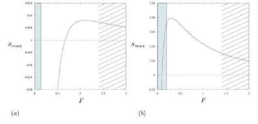
Figure 20: Predicted dimensionless growth rate of the most unstable mode as a function of the Froude number for glass beads ($\theta=29^{\circ}$) ($a$) and sand ($\theta=35^{\circ}$) ($b$) ($\alpha=1$). Grey zone: no flow. Hatched zone: no measurements.

Furthermore, the difference between glass beads and sand becomes clear in the light of the linear stability analysis. The instability mechanism is the same. However, because of quantitative differences in the coefficients of the flow rule, the characteristics of the instability differ in the range where experimental measurements are possible. This is clearly shown in figure 20 where the maximal growth rate predicted by the theory is plotted as a function of the Froude number for both glass beads and sand. We also indicate the range of Froude number where experiments are carried out. It is clear from figure 20 that there is no qualitative difference between both systems. The difference lies only in the relative position of the unstable region compared to the measurement region. For beads the flow threshold is below the instability threshold and the measurements are carried out in a region where the maximum growth rate mainly increases with the Froude number. By contrast, for sand the flow threshold is above the instability threshold and the measurements are carried out in a region where the growth rate decreases with the Froude number.

7 Conclusion

We have presented in this paper an experimental study of the long surface waves instability for dense granular flows down rough inclined planes. By imposing a controlled perturbation at the entrance of the flow, we have been able to precisely measure the threshold and the dispersion relation of the instability.

Using glass beads we have shown that the long-wave instability is controlled by the Froude number and occurs above a critical Froude number. The stability threshold and the velocity of the waves measured experimentally are quantitatively in good agreement with the predictions of a linear stability analysis of the Saint-Venant equations. Using sand, we have observed that the properties of the long-wave instability are strongly modified: the flow is always unstable and the most unstable modes occur for slow flows, near the onset of the flow. Despite the apparent qualitative differences between both systems, we have shown that the wave formation in both cases results from the same instability mechanism and can be described by the stability analysis of the Saint-Venant equations. The difference between sand and glass beads only comes from quantitative differences in the coefficient of the friction law introduced in the Saint-Venant equations.

The instability mechanism for the waves formation in granular flows therefore results, as for classical fluids, from the competition between inertia and gravity. However, the features of the “classical” long-wave instability can be modified due to the specificity of the friction law for granular flows. The most dramatic effect is that the stability threshold may be lowered below the onset of the flow, i.e. a granular flow may be unstable as soon as it flows, when the velocity is small. This property strongly distinguishes granular flows from classical fluid flows and is closely related to the existence of a critical angle in granular material. The existence of a strong instability close to the onset of the flow certainly has dramatic consequences for the non linear evolution of the waves. When the deformations develop, the thickness of the layer can rapidly become less than the minimum thickness needed to flow. The flow then evolves towards a succession of surges separated by material at rest. A similar behavior may be expected for other materials as soon as the material will present a yield stress (mud, clay, granular…). This study then suggests that the existence of surges often observed in geophysical flows could result from the existence of an instability at the onset of flow due to a non zero yield stress condition of the material.

Another interesting result of this study is the relative success of the depth-averaged equations in predicting the stability properties of granular flows. As soon as a relevant friction law is taken into account, quantitative properties can be predicted. This work then provides a good test for the relevance of the friction law deduced from the steady uniform flows, in a case where inertial effects determine the dynamics of the flow.

However, our study reveals an important limitation of the depth-averaged approach we use for describing the instability. The simple first order Saint-Venant equations are unable to predict the cutoff frequency observed in the experiment. This cutoff frequency is the signature of a dissipative mechanism that stabilizes short wavelengths. Since dry granular flows do not experience surface tension, this stabilization mechanism should be related to the streamwise velocity variations that are second order effects in a shallow water description. In order to take into account these longitudinal gradients, one should a priori know the full three-dimensional constitutive equations, which is still an open problem for dense granular flows. Our measurement of the surface wave instability and of the cutoff frequency could therefore serve as a test for future propositions of constitutive equations.

Appendix A

We give in this Appendix the spatial stability analysis of the dispersion relation (12) given by:

$$-\tilde{\omega}^{2}+2\alpha\tilde{\omega}\tilde{k}+\frac{i}{F^{2}}\left((a-b)\tilde{k}-a\tilde{\omega}\right)+\left(\frac{1}{F^{2}}-\alpha\right)\tilde{k}^{2}=0.$$ (28)

The pulsation $\tilde{\omega}$ is real and the wavenumber $\tilde{k}$ is complex: $\tilde{k}=\tilde{k}_{r}+i\tilde{k}_{i}$, the flow is then unstable when $\tilde{k}_{i}\tilde{k}_{r}<0$. The resolution of the dispersion relation (28) gives two spatial modes $(+)$ and $(-)$ for $\tilde{k}(\tilde{\omega})$ that are given by:

$${\tilde{k}_{r}}^{\pm} = \frac{\alpha}{(\alpha-\frac{1}{F^{2}})}\tilde{\omega}\mp\frac{\sqrt{2}(\frac{a}{F^{2}}-\alpha b)}{F^{2}(\alpha-\frac{1}{F^{2}})}\tilde{\omega}{\left[-g(\tilde{\omega})+{\left({g(\tilde{\omega})}^{2}+\frac{16\tilde{\omega}^{2}}{F^{4}}(\frac{a}{F^{2}}-\alpha b)^{2}\right)}^{\frac{1}{2}}\right]}^{-\frac{1}{2}}$$ (29)

$${\tilde{k}_{i}}^{\pm} = \frac{a-b}{2F^{2}(\alpha-\frac{1}{F^{2}})}\mp\frac{1}{2\sqrt{2}(\alpha-\frac{1}{F^{2}})}{\left[-g(\tilde{\omega})+{\left({g(\tilde{\omega})}^{2}+\frac{16\tilde{\omega}^{2}}{F^{4}}(\frac{a}{F^{2}}-\alpha b)^{2}\right)}^{\frac{1}{2}}\right]}^{\frac{1}{2}}$$ (30)

where $g(\tilde{\omega})$ is given by:

$$g(\tilde{\omega})=4\left(\alpha(\alpha-1)+\frac{1}{F^{2}}\right)\tilde{\omega}^{2}-\frac{(a-b)^{2}}{F^{4}}.$$ (31)

For the friction law considered in the article the parameter $a$ is positive and the parameter $b$ is negative. The mode $(-)$ is then always stable whereas the mode $(+)$ may be stable or unstable depending upon the Froude number or the angle of inclination. However it can be shown that the sign of $\tilde{k}_{i}\tilde{k}_{r}$, i.e. the stability of the flow, does not depends upon the pulsation $\tilde{\omega}$. Therefore, to find the stability threshold we can study the asymptotic form of the dispersion relation. For $\tilde{\omega}\to\infty$, one finds:

$${\tilde{k}_{r}}^{\pm}(+\infty) = \frac{\tilde{\omega}}{\alpha\pm\sqrt{\alpha(\alpha-1)+\frac{1}{F^{2}}}},$$ (32)

$${\tilde{k}_{i}}^{\pm}(+\infty) = \frac{\mp a\left(1-\frac{b}{a}-\alpha\mp\sqrt{\alpha(\alpha-1)+\frac{1}{F^{2}}}\right)}{2F^{2}\left(\alpha\pm\sqrt{\alpha(\alpha-1)+\frac{1}{F^{2}}}\right)\sqrt{\alpha(\alpha-1)+\frac{1}{F^{2}}}}.$$ (33)

The mode $(+)$ is then unstable when:

$$1-\frac{b}{a}>\alpha+\sqrt{\alpha(\alpha-1)+\frac{1}{F^{2}}}.$$ (34)

Appendix B

We give here another way to determine the instability condition (15), which underlines the competition between the kinematic waves and the gravity waves in the stability of the flow.

By differentiating (9) with respect to $\tilde{t}$ (resp. with respect to $\tilde{x}$) and (10) with respect to $\tilde{x}$, the perturbed velocity field $u_{1}$ may be eliminated and one obtains a partial linear equation for $h_{1}$ given by:

$$\frac{{\partial}^{2}h_{1}}{\partial\tilde{t}^{2}}+2\alpha\frac{{\partial}^{2}h_{1}}{\partial\tilde{x}\partial\tilde{t}}+(\alpha-\frac{1}{F^{2}})\frac{{\partial}^{2}h_{1}}{\partial\tilde{x}^{2}}=-\frac{a}{F^{2}}\left(\frac{{\partial}h_{1}}{\partial\tilde{t}}+(1-\frac{b}{a})\frac{{\partial}h_{1}}{\partial\tilde{x}}\right),$$ (35)

We then re-write (35) as:

$$\left(\frac{\partial}{\partial\tilde{t}}+\tilde{c}_{+}\frac{\partial}{\partial\tilde{x}}\right)\left(\frac{\partial}{\partial\tilde{t}}+\tilde{c}_{-}\frac{\partial}{\partial\tilde{x}}\right)h_{1}=-\frac{a}{F^{2}}\left(\frac{{\partial}h_{1}}{\partial\tilde{t}}+\tilde{c}_{0}\frac{{\partial}h_{1}}{\partial\tilde{x}}\right),$$ (36)

where $\tilde{c}_{\pm}=\alpha\pm\sqrt{\alpha(\alpha-1)+(1/F^{2})}$ is the speed of the gravity waves upstream and downstream and $\tilde{c}_{0}=1-(b/a)=1+(\partial\tilde{u}/\partial\tilde{h})_{0}$ is the speed of the kinematic waves. Equation (36) reveals waves hierarchy in the system ([Witham 1974]). Long wavelength perturbations propagate to the first order as kinematic waves with a velocity $\tilde{c}_{0}$. The effect of higher order terms may be captured by substituting $\partial/\partial\tilde{t}\sim-\tilde{c}_{0}\partial/\partial\tilde{x}$ on the left-hand side of (36), which leads to:

$$(\tilde{c}_{0}-\tilde{c}_{-})(\tilde{c}_{+}-\tilde{c}_{0})\frac{{\partial}^{2}h_{1}}{\partial\tilde{x}^{2}}=\frac{a}{F^{2}}\left(\frac{{\partial}h_{1}}{\partial\tilde{t}}+\tilde{c}_{0}\frac{{\partial}h_{1}}{\partial\tilde{x}}\right).$$ (37)

This equation is a combined diffusion equation and the stability of the perturbation is given by the sign of the “diffusion coefficient”: $(F^{2}/a)(\tilde{c}_{0}-\tilde{c}_{-})(\tilde{c}_{+}-\tilde{c}_{0})$. For the friction law considered in this paper, $a>0$ and $b<0$, i. e. $\tilde{c}_{0}>1$. On the other hand, $\tilde{c}_{-}<1$ since $\alpha>1$ and $F>0$. Therefore $(\tilde{c}_{0}-\tilde{c}_{-})$ is always positive and the flow is unstable when:

$$\tilde{c}_{0}>\tilde{c}_{+}.$$ (38)

References

- [Ancey 1997] Ancey. C. 1997 Rhéologie des écoulements granulaires en cisaillement simple : application aux laves torrentielles granulaires, Ph.D thesis (Ecole Centrale Paris, Chatenay Malabry, France).
- [Benjamin 1957] Benjamin, T. B. 1957 Wave formation in laminar flow down an inclined plane. J. Fluid Mech. 2, 554-574.
- [Chang 1994] Chang, H-C. 1994 Wave evolution on a falling film. Annu. Rev. Fluid Mech. 26, 103-136.
- [Cornish 1934] Cornish, V. 1934 Ocean waves and kindred geophysical phenomena. Cambridge University Press.
- [Daerr 2001] Daerr, A. 2001 Dynamical equilibrium of avalanches on a rough plane. Phys. Fluids 13, 2115-2124.
- [Daerr & Douady 1999] Daerr, A. & Douady, S. 1999 Two types of avalanche behavior in granular media. Nature 399, 241-243.
- [Davies 1990] Davies, R. H. 1990 Debris-flow surges-experimental simulation. J. Hydrol. (N.Z) 29, 18-46.
- [Douady 1999] Douady, S, Andreotti, B. & Daerr, A. 1999 On granular surface flow equations. Eur. Phys. J. B 11, 131-142.
- [Dressler 1949] Dressler, R. F. 1949 Mathematical solution of the problem of roll-waves in inclined open channels. Communs pure appl. Math. 2, 149-194.
- [Ertas et al 2001] Ertas, D., Grest, G. S., Halsey, T. H., Levine, D. & Silbert, E. 2001 Gravity-driven dense granular flows. Europhys. Lett. 56, 214-220.
- [Gray et al. 1999] Gray, J. M. N. T., Wieland, J. M. & Hutter, K. 1999 Gravity-driven free surface flow of granular avalanches over complex basal topography. Proc. R. Soc. Lond. A455, 573-600.
- [Kapitza & Kapitza 1949] Kapitza, P. L. & Kapitza, S. P. 1949 Wave flow of thin layers of viscous fluid. Zh. Ekper. Teor. Fiz. 19, 105. english traduction in Collected papers of P.L. Kapitza (ed D. Ter Haar), 690-709.
- [Khakhar et al. 1997] Khakhar, D. V., McCarthy, J. J., Shinbrot, T. & Ottino, J. M. 1997 Transverse flow and mixing of granular materials in a rotating cylinder. Phys. Fluids 9, 31-43.
- [Kranenburg 1992] Kranenburg, C. 1992 On the evolution of roll waves. J. Fluid Mech 245, 249-261.
- [Liu et al. 1993] Liu, J., Paul, J. D. & Gollub, J. P. 1993 Measurements of the primary instabilities of film flows. J. Fluid Mech. 250, 69-101.
- [Liu & Mei 1994] Liu, K. & Mei, C. C. 1994 Roll waves on a layer of a muddy fluid flowing down a gentle slope-A Bingham model. Phys. Fluids 6, 2577-2590.
- [Louge & Keast 2001] Louge, M. Y. & Keast, S. C. 2001 On dense granular flows down flat frictional inclines. Phys. Fluids 13, 1213-1233.
- [Naaim et al. 1997] Naaim, M., Vial, S. & Couture, R. 1997 Saint-Venant approach for rock avalanches modeling. In Multiple scale analyses and coupled physical systems: Saint Venant Symposium (Presse de l’École Nationale des Ponts et Chaussées, Paris, 1997).
- [Needham & Merkin 1984] Needham, D. J. & Merkin, J. H. 1984 On roll waves down an open inclined channel. Proc. R. soc. Lond. A 394, 259-278.
- [Oron et al. 1997] Oron, A., Davis, S. & Bankoff, S. G. 1997 Long-scale evolution of thin liquid films. Rev. Mod. Phys. 69 (3), 931-980.
- [Pouliquen & Renaut 1996] Pouliquen, O. & Renaut, N. 1996 Onset of granular flows on an inclined rough surface: dilatancy effects. J. Phys. II France 6, 923–935.
- [Pouliquen ] Pouliquen, O. Scaling laws in granular flows down rough inclined planes. Phys. Fluids 11, 542-548.
- [Pouliquen ] Pouliquen, O. On the shape of granular fronts down rough inclined planes. Phys. Fluids 11, 1956-1958.
- [Pouliquen & Chevoir 2002] Pouliquen, O. & Chevoir, F. 2002 Dense flows of dry granular material. C. R. Physique 3, 163-175.
- [Pouliquen & Forterre 2002] Pouliquen, O. & Forterre, Y. 2002 Friction law for dense granular flows: application to the motion of a mass down a rough inclined plane. J. Fluid Mech. 453, 133-151.
- [Prasad et al. 2000] Prasad, S. N., Pal, D. & Römkens, M. J. M. 2000 Wave formation on a shallow layer of flowing grains. J. Fluid Mech. 413, 89-110.
- [Prochnow et al. 2000] Prochnow, M., Chevoir, F. & Albertelli, M. 2000 Dense granular flows down a rough inclined plane. In Proceedings, XIIIth International Congress on Rheology, Cambridge, UK (2000)
- [Rajchenbach 2000] Rajchenbach, J. 2000 Granular flows. Advances in Physics 49, 229-256.
- [Ruyer-Quil & Manneville 2000] Ruyer-Quil, C. & Manneville, P. 2000 Improved modeling of flows down inclined planes. Eur. Phys. J. B 15, 357-369.
- [Saint-Venant 1871] de Saint-Venant, A. J. C. 1871 Théorie du mouvement non-permanent des eaux, avec application aux crues des rivières et à l’introduction des marées dans leur lit. C. R. Acad. Sc. Paris 73, 147-154.
- [Savage 1979] Savage, S. B. 1979 Gravity flow of cohesionless granular materials in chutes and channels. J. Fluid Mech. 92, 53-96.
- [Savage 1989] Savage, S. B. 1989 Flow of granular materials. in Theoretical and Applied Mechanics, Germain, P., Piau, M. & Caillerie, D. editors., Elsevier, 241-266.
- [Savage & Hutter 1989] Savage, S. B. & Hutter, K. 1989 The motion of a finite mass of granular material down a rough incline. J. Fluid Mech. 199, 177–215.
- [Shkadov 1967] Shkadov, V. Y. 1967 Wave flow regimes of a thin layer of viscous fluid subject to gravity. Izv. Akad. Nauk. SSSR, Mekh. Zhid. Gaza, No. 1, 43-51. (English translation: Fluid Dyn. 2, 29-34.)
- [Simpson 1997] Simpson, J. E. 1997 Gravity currents second ed., Cambridge University Press.
- [Smith 1990] Smith, M. K. 1990 The mechanism for the long-wave instability in thin liquid films. J. Fluid Mech. 217, 469-485.
- [Vallance 1994] Vallance, J. W. 1994 Experimental and field studies related to the behavior of granular mass flows and the characteristics of their deposits, Ph.D Thesis (Michigan Technological University).
- [Vardoulakis 2002] Vardoulakis, I. 2002 Private communication.
- [Wieland et al. 1999] Wieland, J. M., Gray, J. M. N. T. & Hutter, K. 1999 Channelized free-surface flow of cohesionless granular avalanches in a chute with shallow lateral curvature. J. Fluid Mech. 392, 73-100.
- [Witham 1974] Witham, G. B. 1974 Linear and nonlinear waves. Wiley-Interscience.
- [Yih 1963] Yih, C. S. 1963 Stability of liquid flow down an inclined plane. Phys. Fluids 6, 321-330.