A Luttinger Liquid in a Box

Abstract

We study a Luttinger Liquid in a finite one-dimensional wire with box-like boundary conditions by considering the local distribution of the single particle spectral weight. This corresponds to the experimental probability of extracting a single electron at a given place and energy, which can be interpreted as the square of an electron wave-function. For the non-interacting case, this is given by a standing wave at the Fermi wave-vector. In the presence of interactions, however, the wave-functions obtain additional structure with a sharp depletion near the edges and modulations throughout the wire. In the spinful case, these modulations correspond to the separate spin- and charge-like excitations in the system.

The problem of a particle in a one-dimensional box is a classic example in almost any quantum mechanics text-book since it gives a pedagogical introduction to the concept of energy quantization and provides a complete visualization of the corresponding wave-functions. It is however only recently that this problem has gained true experimental relevance due to the progress in constructing smaller and more refined structures to confine electrons in dots and wires. It is for example now possible to resolve the electron wave functions in a finite piece of carbon nanotube by Scanning Tunneling Microscopy (STM) experiments venema ; lemay ; nanotube . Most experimental realizations of one-dimensional electron boxes contain many electrons in a Fermi sea, but it is possible to study a single particle excitation on top of such a ground state configuration and classify the possible energy levels and wave-functions.

However, electron-electron interactions may produce interesting effects in such one-dimensional many-body systems and systematically change the shape of the electron wave-functions. In fact single particle excitations are no longer the eigenstates of an interacting Hamiltonian, but of course it is still interesting to determine the probability of extracting or inserting individual electrons at a given position and energy. This local probability density can be interpreted as the square of the electron wave-function. We therefore study the fundamental problem of single particle excitations in a many body interacting Fermion system confined to a one-dimensional box using the Luttinger Liquid formalism.

We find that the classic example of a box provides again a good visualization of the effect of interactions on the wave-function and the energy quantization. In particular, in addition to the expected rapid Fermi wave-vector oscillations in the wave-function we can recognize long wavelength modulations, which correspond to the underlying boson-like excitations in the Luttinger Liquid. For repulsive interactions the wave-functions are sharply depleted at the edges with a characteristic power-law. Analytic expressions for the wave-functions of the first few levels are presented.

The Luttinger Liquid formalism is a well-established tool to describe interacting electrons confined to one dimension haldane ; senechal . In a linearized region around the Fermi points the Fermion field can be expanded in terms of left- and right-movers

$$\Psi(x,t)\approx e^{ik_{F}x}\psi_{R}(x,t)+e^{-ik_{F}x}\psi_{L}(x,t).$$ (1)

The Fourier modes of the left- and right-moving Fermion density are then represented by bosonic creation and annihilation operators, which effectively act by “shifting” Fermions $m$ steps up or down the spectrum. In the presence of interactions it is then possible to solve the model by a Bogoliubov transformation which mixes the left- and right-moving bosons. This transformation can be described by a single “Luttinger Liquid parameter” $g$, which gives the hyperbolic cosine $\alpha$ and sine $\beta$ of the Bogoliubov transformation

$$\alpha=\frac{1}{2}\left(\frac{1}{g}+g\right),\ \ \ \ \ \beta=\frac{1}{2}\left(\frac{1}{g}-g\right).$$ (2)

Here $g<1$ for repulsive backscattering interactions and $g=1$ for no interactions. Forward scattering does not affect this parameter, but rescales the effective Fermi-velocity.

Let us now consider spinless Fermions in a one-dimensional box of length $L$ with fixed boundary conditions $\Psi(0)=\Psi(L)=0$. After bosonization the Fermion fields become exponentials of the boson operators in a linearized region around the Fermi points

$$\psi_{R}(x,t) = \frac{1}{\sqrt{2\pi a}}e^{i\sqrt{4\pi}(\alpha\phi_{R}(x,t)-\beta\phi_{L}(x,t))}$$ (3)

$$\psi_{L}(x,t) = \frac{1}{\sqrt{2\pi a}}e^{-i\sqrt{4\pi}(\alpha\phi_{L}(x,t)-\beta\phi_{R}(x,t))},$$ (4)

where $a$ is a short-distance cutoff parameter. The fixed boundary condition therefore relates the left- and right-moving boson fields $\phi_{R}(x,t)=-\phi_{L}(-x,t)+\phi_{0}$ and determines the mode expansion in terms of ordinary boson creation and annihilation operators and zero modesgogolin ; mattsson

$$\phi_{L}(x,t)=\frac{\phi_{0}+\tilde{\phi_{0}}}{2}+Q\frac{x+vt}{2L}+\sum_{m=1}^{\infty}\frac{1}{\sqrt{4\pi m}}\left(e^{-i\frac{m\pi}{L}(x+vt)}a_{m}+e^{i\frac{m\pi}{L}(x+vt)}a_{m}^{\dagger}\right)$$ (5)

where $[\tilde{\phi}_{0},Q]=i$ and $\phi_{0}=\frac{\sqrt{\pi}}{2g}$. The eigenvalues of the zero modes $Q=(n-n_{0}-\frac{1}{2})\sqrt{\pi}/g$ are quantized with the number of electrons $n$, where $n_{0}=\frac{k_{F}L}{\pi}$ corresponds to the number of electrons in the ground state.

The Hamiltonian is given by $H=\frac{\pi v}{L}\sum_{m}ma_{m}^{\dagger}a_{m}+\frac{v}{2L}Q^{2}$, where $v$ is the renormalized Fermi velocity. We see that the last term in $H$ resembles a “charging” energy proportional to the square of the excess number of Fermions, but this will not affect our calculations since we always consider single particle excitations with exactly one additional Fermion $n=n_{0}+1$. In general there may also be an additional capacitative energy with a corresponding single particle charging energy $E_{0}$.

The boson excitations become highly degenerate with increasing energy levels which are always quantized $\omega_{m}=m\frac{\pi v}{L}$. However, we are interested in the corresponding Fermion wave-function of a single particle excitation on the ground state $\langle\omega_{m}|x\rangle=\langle\omega_{m}|\Psi^{\dagger}(x)|0\rangle$. The probability density $\rho(\omega_{m},x)$ is given by the sum of the corresponding degenerate wave-functions $\langle\omega_{m}|x\rangle$ squared

$$\rho(\omega_{m},x)\equiv\sum_{\lambda}\left|\langle\omega_{m},\lambda|\Psi^{\dagger}(x)|0\rangle\right|^{2}$$ (6)

This is the local density of states which gives the experimental probability of tunneling an electron into the system at energy $\omega_{m}$ and position $x$. This spectral density can be readily evaluated for an equally-spaced spectrum by the Fourier transformation of the Fermion Green’s function

$$\rho(\omega_{m},x)=\frac{v}{2L}\int_{0}^{2L/v}\!dt\,e^{i\omega_{m}t}\langle\Psi(x,t)\Psi^{\dagger}(x,0)\rangle.$$ (7)

After defining a “mixed wave” $\chi_{m}(x)=\alpha e^{im\frac{\pi x}{L}}+\beta e^{-im\frac{\pi x}{L}}$, we find

$$\langle\psi_{L}(x,t)\psi^{\dagger}_{L}(x,0)\rangle = c\left(\sin{\frac{\pi x}{L}}\right)^{2\alpha\beta}\exp{\left[\sum^{\infty}_{k=1}\frac{e^{-ik\frac{\pi vt}{L}}}{k}|\chi_{k}(x)|^{2}\right]}$$ (8)

$$\langle\psi_{R}(x,t)\psi^{\dagger}_{L}(x,0)\rangle = -c\left(\sin{\frac{\pi x}{L}}\right)^{2\alpha\beta}\exp{\left[\sum_{k=1}^{\infty}\frac{e^{-ik\frac{\pi vt}{L}}}{k}\chi^{2}_{k}(x)\right]}.$$ (9)

Here $c=\frac{4^{2\alpha\beta}}{L}\left(\frac{2\pi a}{L}\right)^{2\beta^{2}}$ is a non-universal cutoff-dependent renormalization parameter which sets the units in our calculations and suppresses the spectral weight in the presence of interactions. These correlation functions can be simplified to powerlaws of sine-functions gogolin ; mattsson ; boundary but the form above avoids any singularities in the integral of Eq. (7) since for a given level $\omega_{m}$ we can truncate the sum in the exponential by $k\leq m$. For the first few levels we are even able to evaluate $\rho$ analytically

$$\rho(\omega_{1},x) = c\left(\sin{\frac{\pi x}{L}}\right)^{2\alpha\beta}2{\rm Im}^{2}\left[\chi_{1}(x)e^{ik_{F}x}\right]$$

$$\rho(\omega_{2},x) = c\left(\sin{\frac{\pi x}{L}}\right)^{2\alpha\beta}\left({\rm Im}^{2}\left[\chi^{2}_{1}(x)e^{ik_{F}x}\right]+{\rm Im}^{2}\left[\chi_{2}(x)e^{ik_{F}x}\right]\right)$$ (10)

$$\rho(\omega_{3},x) = c\left(\sin{\frac{\pi x}{L}}\right)^{2\alpha\beta}\left(\frac{1}{3}{\rm Im}^{2}\left[\chi^{3}_{1}(x)e^{ik_{F}x}\right]+{\rm Im}^{2}\left[\chi_{1}(x)\chi_{2}(x)e^{ik_{F}x}\right]+\frac{2}{3}{\rm Im}^{2}\left[\chi_{3}(x)e^{ik_{F}x}\right]\right)$$

Figure 1: The wave-function squared corresponding to $m=1$ and $n_{0}=40$ in units of $c$. The modulations become more pronounced with increasing interaction strength (smaller g). Last panel: the integrated probability density for the first 50 levels compared to the powerlaw behavior $\omega^{2\beta^{2}}$.

The probability density shows an oscillation of $2k_{F}x$ with modulations according to the mixing of left- and right-moving components in $\chi_{m}$. As can be seen in Fig. 1, the amplitude of the modulations increases with the interaction strength (smaller $g$) and the envelope shows a depletion near the edges with a characteristic powerlaw $x^{2\alpha\beta}$ in agreement with the notion of a boundary exponent gogolin ; mattsson ; boundary ; kane . In the limit of small level spacing $L\to\infty$ we recover the known Luttinger Liquid powerlaw behavior of the integrated density of states $\rho(\omega)\propto\omega^{2\beta^{2}}$ (last panel of Fig. 1). In Fig. 2 we see that the modulations of level $\omega_{m}$ always have $m$ “nodes” and $m+1$ maxima with roughly equal spacing and height resembling a standing wave with a small wave-vector $\omega_{m}/v$, corresponding to the density waves from the boson excitations relative to the Fermi-energy. It is also instructive to consider the non-interacting limit $g=1$, for which we always recover a normalized standing wave of wave-vector $2(k_{F}+\omega_{m}/v)$ without any modulations or depletion, even though a general single Fermion excitation still corresponds to a superposition of degenerate many-boson states (and vice versa).

Figure 2: The wave-function squared of the first few levels for $g=0.7$ and $n_{0}=40$ in units of $c$.

It is now interesting to explore this modulation pattern for the spinful case where we expect separate spin- and charge-like excitations. In this case the electron field with spin $\sigma=\pm$ is expressed in terms of spin and charge boson operators with two Luttinger Liquid parameters $g_{s}$ and $g_{c}$

$$\psi_{R,\sigma}(x)=\frac{1}{\sqrt{2\pi a}}e^{i\sqrt{2\pi}(\alpha_{c}\phi_{R,c}-\beta_{c}\phi_{L,c})}e^{i\sigma\sqrt{2\pi}(\alpha_{s}\phi_{R,s}-\beta_{s}\phi_{L,s})}$$ (11)

and the analogous expression for $\psi_{L,\sigma}$. The mode expansions for the spin and charge bosons are the same as in Eq. (5), and the Hamiltonian is also given by the a simple sum $H=\sum_{\nu=c,s}\left(\sum_{m_{\nu}}\frac{v_{\nu}\pi}{L}m_{\nu}a^{\dagger}_{m_{\nu}}a_{m_{\nu}}+\frac{v_{\nu}Q_{\nu}^{2}}{2L}\right)$.

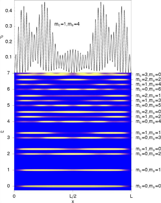
Figure 3: The single particle density of a spinful interacting electron system as a function of energy and position along a finite box for $g_{s}=0.7,\ g_{c}=0.6$, and $v_{c}=2.3v_{s}$ (slightly broadened, so that the fast oscillations are averaged out). This may resemble the outcome of a $dI/dV$ measurement in an STM experiment on a finite interacting wire. Top: fully resolved level for $m_{s}=4,\ m_{c}=1$, and $\frac{k_{F}L}{\pi}=40$. The two charge peaks and the five weaker spin peaks are visible.

Therefore, the spin and charge excitations are decoupled except for the quantization conditions on the zero modes $Q_{s}=\frac{\sqrt{\pi}}{\sqrt{2}g_{s}}l$, $Q_{c}=\frac{\sqrt{\pi}}{\sqrt{2}g_{c}}\left(n-1-\frac{2k_{F}L}{\pi}\right)$ that $[l,n]$ must be either both even or both odd ([1,1] in our case). For the non-interacting case, spin- and charge-excitations are exactly degenerate, but now the excitations are classified by the product space of two evenly spaced boson spectra with different energy spacing $v_{s}<v_{c}$. The partition function and the electron Green s function factorize. Therefore, the wave-functions are products of spin- and charge-modulations which are similar to the ones shown in Fig. 2 and Eq. (10), except that the mixed wave is rescaled $\chi_{m,\nu}(x)=\frac{\alpha_{\nu}}{\sqrt{2}}e^{im\frac{\pi x}{L}}+\frac{\beta_{\nu}}{\sqrt{2}}e^{-im\frac{\pi x}{L}},\ \nu=s,c$ and the overall factor is given by $\left(\sin{\frac{\pi x}{L}}\right)^{\alpha_{s}\beta_{s}}\left(\sin{\frac{\pi x}{L}}\right)^{\alpha_{c}\beta_{c}}$.

In Fig. 3 we show the square of the wave-functions at the lowest energies in a spinful interacting electron system with $g_{s}=0.7,\ g_{c}=0.6$, and $v_{c}=2.3v_{s}$. Due to the different velocities, the degeneracy is lifted and many more levels appear as the energy is increased [see also Fig. 4 in Ref. mattsson ]. Each level is classified by a spin and a charge quantum number $m_{s}$ and $m_{c}$, which is reflected by the corresponding number of nodes and maxima in the wave-functions. For example the level $m_{s}=4,\ m_{c}=1$ shows a superposition of two charge maxima and five weaker spin maxima. In Fig. 3 we have chosen values of $g_{s}=0.7$ and $g_{c}=0.6$, which emphasizes the locations of both spin and charge modulations, but in systems where the interactions are mostly spin-independent $g_{s}$ is likely to be much closer to unity and the spin modulations are less pronounced. Nonetheless, the level structure due to $v_{s}<v_{c}$ as well as the charge modulations are likely to be observable when classifying Luttinger Liquid systems in real space with STM experiments.

The integrated weight of the individual levels decreases with increasing energy, but the total (averaged) density of states increases with the known powerlaw $\rho(\omega)\propto\omega^{\beta_{s}^{2}+\beta_{c}^{2}}$. The superstructures survive even in the continuum limit and give rise to the observed slow oscillations with wave-vectors $\omega/v_{c}$ and $\omega/v_{s}$ near the edge of a semi-infinite Luttinger Liquid mattsson ; boundary ; stm ; meden . In the non-interacting limit $g_{s}=g_{c}=1$ we recover again standing waves with a fixed wave-vector without any modulations, and remarkably all the many degenerate spin and charge boson states at each energy level exactly sum up to an integrated normalized spectral weight of unity.

In conclusion we have shown that the single particle wave-functions of interacting Fermions in a box can be used to visualize the true nature of the underlying boson excitations. Given the rapid progress in STM imaging and nano-structured materials this may soon be observable when classifying different kinds of potential Luttinger Liquid systems.

This research was supported in part by the Swedish Research Council and INFM.

References

- (1) L.C. Venema, et al., Science 283, 52 (1998).
- (2) S.G. Lemay, et al., Nature 412, 617 (2001).
- (3) Due to the metallic substrates, interaction effects are screened in the two experiments venema ; lemay .
- (4) F.D.M. Haldane, J. Phys. C: Solid State Phys. 14, 2585 (1981).
- (5) For a compact review see D. Sénéchal, preprint cond-mat/9908262 (unpublished).
- (6) M. Fabrizio and A.O. Gogolin, Phys. Rev. B 51, 17827 (1995).
- (7) A.E. Mattsson, S. Eggert and H. Johannesson, Phys. Rev. B 56, 15615 (1997).
- (8) S. Eggert, H. Johannesson, and A. Mattsson, Phys. Rev. Lett. 76, 1505 (1996).
- (9) C.L. Kane and M.P.A. Fisher, Phys. Rev. Lett. 68, 1220 (1992).
- (10) S. Eggert, Phys. Rev. Lett. 84, 4413 (2000).
- (11) V. Meden et al., Eur. Phys. J. B 16, 613 (2000).