Defect turbulence and generalized statistical mechanics

Abstract

We present experimental evidence that the motion of point defects in thermal convection patterns in an inclined fluid layer is well-described by Tsallis statistics with an entropic index $q\approx 1.5$. The dynamical properties of the defects (anomalous diffusion, shape of velocity distributions, power law decay of correlations) are in good agreement with typical predictions of nonextensive models, over a range of driving parameters.

1 Introduction

In recent years a generalized version of statistical mechanics proposed by C. Tsallis, dubbed nonextensive statistical mechanics [1, 2, 3], has been subject to intensive discussion [4]. The basic idea underlying this new theoretical approach is quite simple: suppose that a physical system of sufficient complexity cannot, for some reason, maximize the usual Boltzmann-Gibbs-Shannon entropy leading to the usual statistical mechanics. In such a case, it is reasonable to conjecture that the system may then maximize some other, more general entropy measure. In particular, good candidates for such measures are the Tsallis entropies $S_{q}$, which depend on a real parameter $q$, the entropic index. If $q\neq 1$, the Tsallis entropies are nonextensive, i.e. nonadditive for independent subsystems. For $q=1$, they reduce to the Boltzmann entropy and the usual statistical mechanics is recovered.

If the Tsallis entropies are maximized subject to suitable constraints, one arrives at power-law generalizations for the canonical ensemble, with $q$ being related to the exponent of the power law. An important (and open) question involves determining for which types of systems this more general formalism is physically relevant. We can imagine various reasons why a particular physical system may not be able to maximize the usual Boltzmann entropy: long-ranged interactions/correlations, multifractality, metastability, or simply the fact that the system is not in equilibrium due to some external forcing. Indeed, recent work has shown that nonextensive statistical mechanics is particularly useful in describing driven nonequilibrium systems. Useful physical applications include Eulerian [5, 6] and Lagrangian [7, 8] fully-developed hydrodynamic turbulence, heavy ion collisions [9], $e^{+}e^{-}$ annihilation experiments [10, 11], as well as economic [12] and biological [13] systems.

Here we report experimental observations of point defect (dislocation) motion in defect turbulence in inclined layer convection [14, 15], which are found to be consistent with Tsallis statistics. To the best of our knowledge, this is the first observation of Tsallis statistics in a defect turbulent pattern-forming system. The defects behave much like particles obeying a generalized Tsallis-type statistical mechanics, with an entropic index of approximately $q\approx 1.5$. Their dynamical properties (anomalous diffusion, skewness, power law decay of correlations) are in good agreement with typical predictions of nonextensive models over a range of driving parameters. In addition, since this system is but one of many driven systems exhibiting defect turbulence, these findings suggest that similar non-extensive behavior may be found in other pattern-forming systems such as electroconvection in liquid crystals [16], nonlinear optics [17], and auto-catalytic chemical reactions [18].

2 Experiment

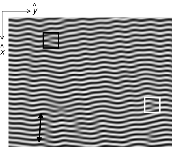
Figure 1: Example shadowgraph image of undulation chaos in fluid layer heated from below and cooled from above, inclined by an angle $\theta=30^{\circ}$. The nondimensional driving paramter is $\epsilon=0.08$. Black box encloses a positive defect; white, a negative. Arrow is adjacent to a tearing region of low-amplitude convection. Uphill direction is at left side of page. Region shown is the subregion of size $51d\times 63d$ used for analysis.

We examine the motion of defects within spatiotemporally chaotic patterns formed in experiments on inclined layer convection (ILC), a variant of Raleigh-Bénard convection [19] in which the thin fluid layer (heated from below and cooled from above) is inclined by an angle $\theta$ from the horizontal [14]. For intermediate angles of inclination ($15^{\circ}<\theta<75^{\circ}$ at Prandtl number $\approx 1$), the system exhibits defect turbulence within a pattern of undulating convection rolls. This state is known as undulation chaos [14, 15]; an example is shown in Fig. 1, with defects marked by boxes and a tearing region marked by an arrow.

The experimental apparatus and data collection for this investigation have previously been discussed in [14, 15], and only key points are summarized here. The planform of the convection pattern was obtained using the shadowgraph technique [20] and a digital camera. The fluid used was compressed CO₂ with Prandtl number ${\mathrm{P}r}=\nu/\kappa\approx 1$, where $\nu$ is the kinematic viscosity and $\kappa$ is the coefficient of thermal expansion. The convection cell had a thickness of $d=(388\pm 2)\mu$m and was of dimension $101d\times 50d$, of which only a central $51d\times 63d$ region was used for analysis. The vertical thermal diffusion time was $\tau_{v}=d^{2}/\kappa=1.53$ sec. All data was collected at an inclination of $\theta=30^{\circ}$. The strength of the thermal driving is described by the nondimensional temperature difference $\epsilon\equiv\frac{\Delta T}{\Delta T_{c}}-1$; this quantity was varied in the experiments. Data collection occurred at 3 frames/sec in two modes: four to six hundred 100-frame runs at each of 17 values of $0.04\leq\epsilon\leq 0.22$ and a few (4, 2 respectively) 80,000-frame runs at $\epsilon=0.08$ and $\epsilon=0.17$. Each value of $\epsilon$ was reached via quasistatic temperature changes. We also conducted a sequence of measurements with quasistatic temperature increases followed by quasistatic temperature decreases to check for possible hysteresis, which was not observed. The Boussinesq parameter [19] was $Q=0.8$, indicating a breaking of the up-down ($\hat{z}$) symmetry.

Due to the inclination of the fluid layer, the system is anisotropic and the convection roll axes align along the direction of the shear flow ($\hat{y}$) for intermediate inclinations such as $\theta=30^{\circ}$. In contrast to what is observed in Rayleigh-Bénard convection, the defect motion is observed to be primarily transverse to the convection rolls (“glide,” in the language of crystals) instead of parallel (“climb”). As such, the motion of the defects does not typically adjust the local wavenumber of the rolls, rather their orientation and the wavenumber of the undulations.

3 Nonextensive statistical mechanics of defects

3.1 Observed defect statistics

Topological defects in spatiotemporally chaotic patterns such as undulation chaos in ILC behave much like particles: they have charge; they are created and annihilated; and they have a well-defined position and velocity. Their topological charge is a quantity analogous to a Burger’s vector; point defects (dislocations) are located at positions where there is a discontinuity of $\pm 2\pi$ in the phase of the pattern $\Phi$ along a contour around the point:

$$\oint\vec{\nabla}\Phi\cdot d\vec{s}=\pm 2\pi,$$ (1)

As seen in Fig. 1, undulation chaos consists of an underlying set of stripes (convection rolls) which contain both undulations and such defects. Each of these features is observed to be spatiotemporally chaotic. While undulation chaos has strong nonequilibrium properties due to the thermal forcing, it nonetheless exhibits stationarity in distributions of the number of defects and the wavenumber [14].

If the defects behaved like an ideal gas obeying standard statistical mechanics, the probability $P_{N}$ to observe $N$ particles in a certain area would be given by the Poisson distribution $P_{N}=\frac{e^{-\lambda}\lambda^{N}}{N!}$ where $\lambda$ is the average number of particles. However, this distribution has been observed to be invalid for a number of defect turbulent systems [21, 14, 22]. A particular model for $P_{N}$, based on empirically determined rate equations, has been studied in [14]. It yields a modified Poisson distribution

$$P_{N}=\frac{a^{(b/2)+N}}{I_{b}(2\sqrt{a})\Gamma(1+b+N)N!}$$ (2)

where $I_{b}$ denotes the modified Bessel function and the constants $a$ and $b$ are determined by the defect gain and loss rates. This prediction differs significantly in its variance from the Poisson distribution, and agrees very well with the experimentally observed distributions in undulation chaos [14].

Besides defect number, it is also interesting to look at the statistics of defect velocities. We examine the ensemble of defect trajectories decomposed into the two directions $\hat{x}$ (across rolls) and $\hat{y}$ (along rolls, uphill-downhill) coinciding with the anisotropy of the system. This decomposition is done because their motions are fundamentally different with respect to the underlying roll structure; their dynamics have been observed to evolve in a nearly statistically independent way [15]. If the defects behaved like ordinary particles obeying ordinary statistical mechanics, one would expect Gaussian velocity distributions and normal diffusion of the positions. Instead, significant deviations are observed [15].

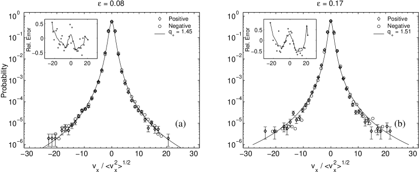
Figure 2: Transverse velocity ($v_{x}$) distributions at (a) $\epsilon=0.08$ and (b) $\epsilon=0.17$ for positive and negative defects, rescaled to $\sigma=1$. Solid lines are one-parameter fits to Eq. (6) for positive defects. Unrescaled standard deviations were: (a) $\sigma_{+}=0.550$, $\sigma_{-}=0.553$ and (b) $\sigma_{+}=0.586$, $\sigma_{-}=0.565$. Inset: Relative error of experiment and theory: $(p_{exp}-p_{theory})/p_{theory}$.

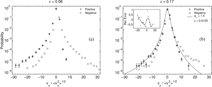
Figure 3: Longitudinal velocity ($v_{y}$) distributions at (a) $\epsilon=0.08$ and (b) $\epsilon=0.17$ for positive and negative defects, rescaled to $\sigma=1$. Solid line is a fit to Eq. (10) for positive defects. Unrescaled standard deviations were: (a) $\sigma_{+}=0.099$, $\sigma_{-}=0.115$ and (b) $\sigma_{+}=0.141$, $\sigma_{-}=0.128$. Inset: Relative error of experiment and theory: $(p_{exp}-p_{theory})/p_{theory}$.

The probability density functions (PDFs) of the velocities $v_{x}$ and $v_{y}$ are shown in Fig. 2 and 3, with velocities rescaled by their standard deviation $\sigma$. Data is shown for $\epsilon=0.08$ and 0.17, the two values with the largest datasets. The PDFs deviate significantly from a Gaussian, with velocities of more than $20\sigma$ observed in the long tails. In the transverse direction ($\hat{x}$), the velocities are several times faster than those in in the longitudinal ($\hat{y}$) direction.

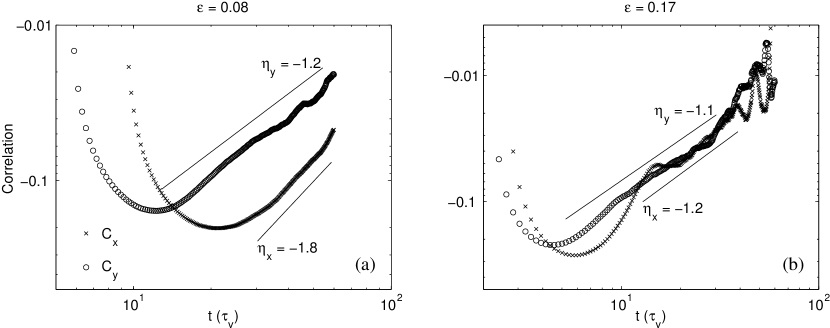
Figure 4: Tails of velocity autocorrelation functions for $v_{x}$ ($\times$) and $v_{y}$ ($\circ$) at (a) $\epsilon=0.08$ and (b) $\epsilon=0.17$. Straight lines indicate fits to power laws. These curves are the tails of the results shown in Fig. 4 of [15].

A common characteristic of nonextensive systems is the presence of long-range interactions and/or long-range correlations: for generic nonextensive models, velocity correlation functions are expected to decay asymptotically with a power law. While the temporal correlation function $C(t)$ of defect velocities decays exponentially for small $t$ ($<10\tau_{v}$) [15], Fig. 4 reveals a superimposed long-term power law contribution of the form $C(t)\sim t^{-\eta}$ for large $t$. For both $v_{x}$ and $v_{y}$ at both values of $\epsilon$, the exponent $\eta$ is greater than 1, although the fit region is of limited length due to finite observation times.

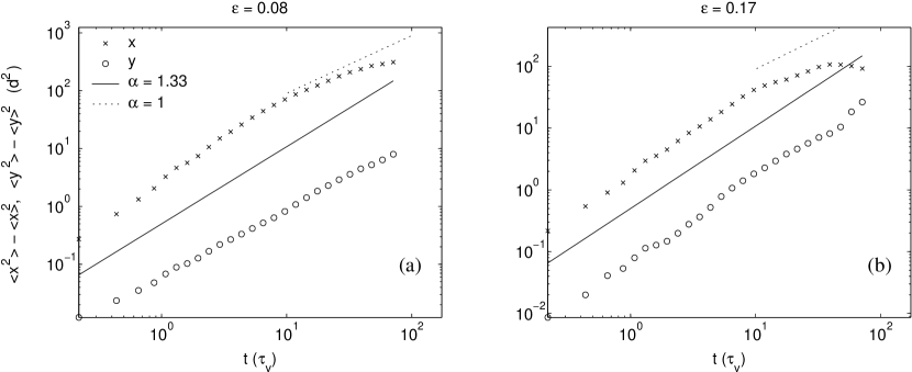
Figure 5: Second moment of position trajectories in $\hat{x}$ and $\hat{y}$. Solid line is diffusive behavior predicted by Eq. (18) for $q=1.5$; dotted line is normal diffusive limit ($q=1$).

Finally, these observed velocities provide for defect diffusion. Normal diffusive behavior is given by the second moment of the position $\langle x(t)^{2}\rangle-\langle x(t)\rangle^{2}\propto t^{\alpha}$ where $\alpha=1$ and $\langle\cdot\rangle$ represents an ensemble-average. Defect motion in undulation chaos exhibits superdiffusive behavior in both $\hat{x}$ and $\hat{y}$, as shown in Fig. 5, where the exponent $\alpha$ is greater than 1.

3.2 Generalized canonical distributions

Given this anomalous behavior, we investigate the proposition that the defects obey a generalized statistical mechanics of the Tsallis type and work out the corresponding predictions. Because the number of defects is not constant but fluctuates, such fluctuations should properly be embedded into a generalized grand canonical description. To date, however, no general theory of the nonextensive grand canonical ensemble is known, and we instead use the canonical nonextensive model. This theory predicts that the stationary PDF of an observable $u$ should be given by the generalized canonical distribution

$$p(u)=\frac{1}{Z_{q}}(1+(q-1)\tilde{\beta}E(u))^{-\frac{1}{q-1}}.$$ (3)

Here $E(u)$ is an effective energy associated with $u$, and

$$Z_{q}=\int_{-\infty}^{+\infty}(1+(q-1)\tilde{\beta}E(u))^{-\frac{1}{q-1}}du$$ (4)

is a normalization constant. $\tilde{\beta}=1/(kT)$ is a (formal) inverse temperature variable, which essentially fixes the variance of the distributions, and $q$ is the entropic index.

The distribution in Eq. (3) is obtained by maximizing the Tsallis entropies

$$S_{q}=\frac{1}{q-1}\left(1-\sum_{i}p_{i}^{q}\right),$$ (5)

subject to suitable constraints [1, 2]. The $\{p_{i}\}$ are the probabilities of the microstates $i$ of the system. In the limit $q\to 1$, the usual Boltzmann distribution is recovered from Eq. (3).

The lowest-order model is $E(u)=\frac{1}{2}u^{2}$, which may be associated with an effective kinetic energy. For this relation, one obtains the PDF

$$p(u)=\frac{1}{Z_{q}}\left(1+\frac{1}{2}(q-1)\tilde{\beta}u^{2}\right)^{-\frac{1}{q-1}},$$ (6)

where

$$Z_{q}=\sqrt{\frac{2}{(q-1)\tilde{\beta}}}\cdot\frac{\Gamma(\frac{1}{2})\Gamma(\frac{1}{q-1}-\frac{1}{2})}{\Gamma(\frac{1}{q-1})}.$$ (7)

The distribution in Eq. (6) has variance 1 if $\tilde{\beta}$ is chosen to be

$$\tilde{\beta}=\frac{2}{5-3q}$$ (8)

yielding a single fit parameter $q$.

In general, however, defect interactions, the local pattern, and other higher-order correlations of the chaotic forces acting on the defects will produce small correction terms to $E(u)$. The effect of such higher-order correlations of chaotic driving forces has been studied in [23, 24]. The result of those considerations is that for distributions which have been rescaled to $\sigma=1$ the effective energy is of the form

$$E(u)=\frac{1}{2}u^{2}+c\left(u-\frac{1}{3}u^{3}\right)+O(c^{2}).$$ (9)

Here $c$ is a small constant related to the skewness of the distribution and whether or not it is nonzero depends on the universality class of the chaotic driving forces that are acting. Eq. (9) is a perturbative result that is valid for $u\ll c^{-1}$. Neglecting higher-order corrections of $O(c^{2})$ we obtain the formula

$$p(u)=\frac{1}{Z_{q}}\left(1+\tilde{\beta}(q-1)\left(\frac{1}{2}u^{2}-c(u-\frac{1}{3}u^{3})\right)\right)^{-\frac{1}{q-1}}$$ (10)

for the probability distribution.

When this formalism is applied to defects, we associate $u$ with either $v_{x}$ or $v_{y}$, rescaled by $\langle v_{x,y}^{2}\rangle^{1/2}$ to obtain an appropriate dimensionless quantity. Conceptually, this corresponds to associating the $u^{2}$ term of $E(u)$ with an effective “kinetic energy,” in the language of ideal gases. In the case of the transverse motion ($\hat{x}$, Fig. 2) of the defects, the measured PDFs are symmetric and coincide very well with symmetric ($c=0$) Tsallis distributions of the form Eq. (6), while for the $\hat{y}$ motion (Fig. 3) significant asymmetries are present and Eq. (9) is appropriate with $c\neq 0$. The presence of this skewness in the $v_{y}$ may be associated with the non-Boussinesqness of the fluid flow, which causes the shear flow to be asymmetric in $\hat{z}$. Previous studies of inclined layer convection [14] have revealed similar asymmetries: the undulations drift in the $\hat{y}$ direction.

We fit the experimentally obtained PDFs to either Eq. (6) or (10) by minimizing $\sum(p_{exp}-p_{theory})^{2}/p_{theory}$, which allows for appropriate weighting of the tails. These fits can be seen as the solid lines in Figs. 2 and 3. For $v_{x}$, we obtained values of $q=1.45$ at $\epsilon=0.08$ and $1.51$ at $\epsilon=0.17$, with the value for $\tilde{\beta}$ set via Eq. (8) by rescaling the distributions to $\sigma=1$. For $v_{y}$, we find $q=1.40$ and $c=0.0125$ (such that the expansion is valid for $u\ll 80$) at $\epsilon=0.17$. For $v_{y}$ at $\epsilon=0.08$, the data is sufficiently skewed to violate the conditions under which the expansion in $c$ is valid, and no good fit was found even for values of $c>0.03$. It should be noted that these fits do display small systematic deviations from the data, which may or may not be significant over six orders of magnitude.

The PDFs for the velocity components are not significantly changing in $q$, $\tilde{\beta}$, and $c$ across the values of $\epsilon$ surveyed. This is demonstrated in Fig. 6 for $v_{x}$ and $v_{y}$ in which the PDFs are found to coincide with no rescaling. Fig. 7 shows the fit values for $q$ and $c$ at various $\epsilon$. A mean value of $\bar{q}=1.48\pm 0.05$ is observed for $v_{x}$. For $v_{y}$, we observe $\bar{q}=1.51\pm 0.15$ and $\bar{c}=0.012\pm 0.002$ (with the sign of $c$ corresponding to the sign of the defect). Remarkably, the distributions are constant in spite of a transition [15] from disordered undulations for $\epsilon\lesssim 0.1$ to intermittently ordered undulations for $\epsilon\gtrsim 0.1$.

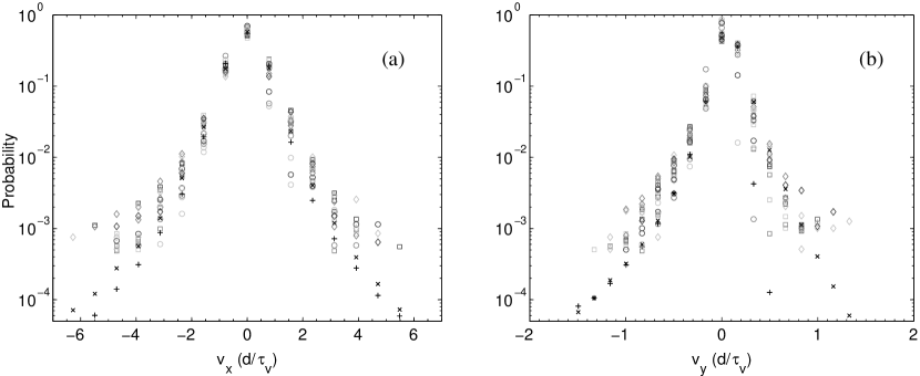
Figure 6: Overlay of (a) $v_{x}$ PDFs and (b) $v_{y}$ PDFs for positive defects at 17 values of $\epsilon$ (open, gray symbols) with data at $\epsilon=0.08$ ($+$) and $\epsilon=0.17$ ($\times$). This data corresponds to the peak region of Figs. 2 and 3, but not rescaled by $\sigma$.

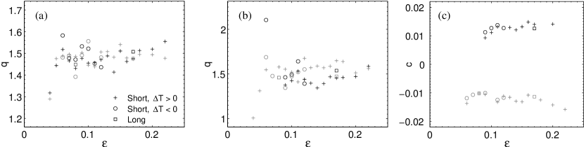
Figure 7: Values of fit parameters (a) $q$ for $v_{x}$ (b) $q$ for $v_{y}$, and (c) $c$ for $v_{y}$ as a function of $\epsilon$. Data in black is for positive defects; data in gray is for negative. Short runs in which data was obtained by quasistatic temperature increases from below are marked with $+$, and the converse with $\circ$.

3.3 Effective degrees of freedom of the environment

We now consider concrete dynamical models exhibiting nonextensive behavior. One of the simplest models, described in [6], is a linear Langevin equation whose friction parameter is also stochastic. We use such an equation as a simplified dynamical model for defect velocities:

$$\dot{u}=-\gamma(\vec{x},t)u+\kappa L(t),$$ (11)

where $L(t)$ is Gaussian white noise of strength $\kappa$ and $\gamma(\vec{x},t)$ is a random damping constant which fluctuates and may be attributed to spatiotemporal changes in the environment of the defect. One can let $\kappa$ fluctuate as well [6], but this is not necessary for our purposes.

It has been shown in [6] that Eq. (11) generates Tsallis distributions for $u$ if $\beta\equiv\gamma/\kappa^{2}$ is $\chi^{2}$-distributed with degree $n$, i.e. if the PDF of $\beta$ is given by

$$f(\beta)=\frac{1}{\Gamma(\frac{n}{2})}\left(\frac{n}{2\beta_{0}}\right)^{\frac{n}{2}}\beta^{\frac{n}{2}-1}\exp\left[-\frac{n\beta}{2\beta_{0}}\right].$$ (12)

Such a distribution is generated by a sum of $n$ Gaussian random variables $X_{i}$, squared:

$$\beta=\sum_{i=1}^{n}X_{i}^{2}$$ (13)

If $\beta$ fluctuates on a time scale that is much larger than the relaxation time to reach local equilibrium, then, as shown in [6], Eq. (11) generates stationary densities of the form (6) with

$$q=1+\frac{2}{n+1},$$ (14)

$$\tilde{\beta}=\frac{2}{3-q}\beta_{0}.$$ (15)

Here $\beta_{0}=\int_{0}^{\infty}f(\beta)\beta~{}d\beta$ is the average value of the fluctuating $\beta$. The experimentally observed value $q\approx 1.5$ for the defect statistics thus means that there are effectively 3 independent degrees of freedom that contribute to the fluctuating local defect environment.

Defects are no ordinary particles: they have neither a well-defined mass nor a well-defined size. Furthermore, the nature of defect turbulence means that they are moving within a spatiotemporally chaotic environment. Therefore, one expects that there is an ensemble of damping constants which depend on the environment of the defect, providing the fluctuating effective damping $\gamma$.

In particular, the fastest velocities result from circumstances in which the defect is moving in a local environment corresponding to weak damping (small $\gamma$). In undulation chaos, such events coincide with the presence of a transverse region of low-amplitude convection, as shown by the black arrow in Fig. 1. The rapid motion takes place due to the fact that the pattern “tears” in such a way that each roll broken rejoins with the one next to it, rapidly transporting the defect across the weak region. The driving forces $L(t)$ are weakly damped during such a time interval, leading to very large velocities for short intervals, until another region with another $\gamma$ is reached. The behavior of such flight-like events is further described in [15].

In general, one may also consider probability distributions other than the $\chi^{2}$-distribution in used Eq. (12). These lead to statistics other than Tsallis statistics: superstatistics [25], for which generalized versions of statistical mechanics can be constructed as well [26]. Using these extensions, it can been shown that for $\beta$-fluctuations of small variance and not too large $|u|$ all superstatistics are universal, and in fact are given by Tsallis statistics [25]. Significant differences arise only for large $|u|$. In general, the $\chi^{2}$-distribution is distinguished by the fact that it yields a superstatistics whose generalized entropies have “better” properties than those of other superstatistics.

3.4 Anomalous diffusion

Typical nonextensive models predict anomalous diffusion, such that

$$\langle x(t)^{2}\rangle-\langle x(t)\rangle^{2}\propto t^{\alpha}$$ (16)

with $\alpha\neq 1$, as is observed in the diffusion of defects in undulation chaos. The nonlinear Fokker-Planck model previously discussed in [27, 28] describes correlated anomalous diffusion in the framework of nonextensive models. It is based on a generalized Fokker-Planck equation of the form

$$\frac{\partial}{\partial t}p(x,t)=-\frac{\partial}{\partial x}\left(F(x)p(x,t)\right)+D\frac{\partial^{2}}{\partial x^{2}}(p(x,t))^{\nu}$$ (17)

with a linear drift term given by $F(x)=k_{1}-k_{2}x$.

The linear case ($\nu=1$) corresponds to the standard Fokker-Planck equation generating the usual Brownian motion processes with Gaussian densities. As shown in [27], the nonlinear case where $\nu\neq 1$ generates Tsallis distributions, with the entropic index $q$ being related to the parameter $\nu$ by $q=2-\nu$. In addition, the model generates anomalous diffusion for $\nu\neq 1$, with the relation between the exponent $\alpha$ of anomalous diffusion and the entropic index $q$ given by [27]

$$\alpha=\frac{2}{1+\nu}=\frac{2}{3-q}.$$ (18)

Thus, we can compare the results for the Tsallis fits to the PDFs and the exponents in the diffusion graphs. Remarkably, the value $\alpha=1.33$ obtained from Eq. (18) for $q=1.5$ provides a good match to the observed data. Other models, based on 2-dimensional Levy flights [29], predict $\alpha=q-1\approx 0.5$ and are apparently not consistent with our data. This can be understood within the framework described here: we earlier found that $n\approx 3$, which means that there are effectively more than 2 degrees of freedom contributing to the fluctuating environment of the defect.

3.5 Velocity correlation function

To better understand the relationship between Figs. 4 and 5, we can perform a simplified calculation relating the velocities and positions. To do so, we neglect all spatial correlations, which do effect the diffusion but have not been measured, and focus only on the temporal ones. In each spatial direction the displacements obey $x(t)\equiv\int_{0}^{t}v(t^{\prime})dt^{\prime}$. Hence,

$$\langle x^{2}(t)\rangle = \int_{0}^{t}dt^{\prime}\int_{0}^{t}dt^{\prime\prime}\langle v(t^{\prime})v(t^{\prime\prime})\rangle$$ (19)

$$= 2\int_{0}^{t}dt^{\prime}\int_{0}^{t^{\prime}}d\tau\langle v(0)v(\tau)\rangle.$$ (20)

Assuming the simple asymptotic form $\langle v(0)v(\tau)\rangle\sim\tau^{-\eta}$, the two integrations in Eq. (20) yield

$$\langle x^{2}(t)\rangle\sim t^{-\eta+2},$$ (21)

as the expected behavior in the asymptotic limit. By equating this expression with Eq. (16), one obtains a relation between $\eta$ (describing the velocity autocorrelation) and $\alpha$ (describing the diffusion), namely

$$\eta=2-\alpha.$$ (22)

In the experimental data displayed in Fig. 5, we observed that the effective anomalous diffusion exponent $\alpha$ is given by $\alpha\approx 1.33$ on moderate time scales and decreases to $\alpha\lesssim 1$ for large time scales $t>10\tau_{v}$. Thus, Eq. (22) yields $\eta\approx 2-\alpha\gtrsim 1$ for the long-term decay exponent of the velocity correlation function. As Fig. 4 shows, this is in good agreement with the measured decay rate of the velocity autocorrelation function.

4 Conclusions

We have provided experimental evidence that topological defects in Inclined Layer Convection behave in a similar fashion to an ideal gas of nonextensive statistical mechanics with $q\approx 1.5$. This is an application to a physical system far from equilibrium, where the standard statistical mechanics has little to say. Not only do the measured probability distributions of defect velocities agree well with Tsallis statistics, but we find quantitative agreement in the nonextensive parameter $q\approx 1.5$ as determined from both velocity distributions and diffusive behavior.

While the direct observation of nonextensive behaviour of the entropy may not be possible , further work may nonetheless be able to provide a prediction for $q$. One promising approach would be to quantify the fluctuations in $\beta$, the environment of the defect, in terms of observed pattern properties such as local wavedirector and convection amplitude. If so, then the recent superstatistics described in [25] could provide a suitable framework. Furthermore, other defect-turbulent systems may also exhibit similar behavior and prove a fertile ground for further investigations.

KED and EB are grateful to the National Science Foundation for support under DMR-0072077.

References

- [1] C. Tsallis, J. Stat. Phys., 52: 479 (1988)
- [2] C. Tsallis, R.S . Mendes and A. R. Plastino, Physica, 261A: 534 (1998)
- [3] S. Abe, Y. Okamoto (eds.), Nonextensive Statistical Mechanics and Its Applications, Berline: Springer (2001)
- [4] A. Cho, Science, 297: 1268 (2002)
- [5] C. Beck, G. S. Lewis, H. L. Swinney, Phys. Rev. E, 63: 035303R (2001)
- [6] C. Beck, Phys. Rev. Lett., 87: 180601 (2001)
- [7] C. Beck, Phys. Lett. A, 287: 240 (2001)
- [8] G. A. Voth, et al., J. Fluid Mech., 469: 121 (2002)
- [9] W. M. Alberico, A. Lavagno, P. Quarati, Eur. Phys. J., C12: 499 (2000)
- [10] I. Bediaga, E. M. F. Curado, J. M. de Miranda, Physica, 286A: 156 (2000)
- [11] C. Beck, Physica, 286A: 164 (2000)
- [12] L. Borland, Phys. Rev. Lett., 89: 098701 (2002)
- [13] A. Upadhyaya, J.-P. Rieu, J. A. Glazier, Y. Sawada, Physica, 293A: 549 (2001)
- [14] K. E. Daniels, E. Bodenschatz, Phys. Rev. Lett., 88: 034501 (2002)
- [15] K. E. Daniels, E. Bodenschatz, Chaos, 13: 55 (2003)
- [16] I. Rehberg, S. Rasenat, and V. Steinberg, Phys. Rev. Lett., 62: 756 (1989).
- [17] P. Ramazza, S. Residori, G. Giacomelli, and F. Arecchi, Europhys. Lett., 19: 475 (1992).
- [18] Q. Ouyang and J. M. Flesselles, Nature, 379: 143 (1996).
- [19] G. Ahlers, E. Bodenschatz, W. Pesch, Annu. Rev. Fluid Mech., 32: 709 (2000)
- [20] J. R. de Bruyn et al., Rev. Sci. Instrum., 67: 2043 (1996)
- [21] L. Gil, J. Lega, J. L. Meunier, Phys. Rev. A, 41: 1138 (1990)
- [22] Y.-N. Young, H. Riecke, physics/0209062
- [23] A. Hilgers and C. Beck, Phys. Rev. E, 60: 5385 (1999)
- [24] C. Beck, Physica, 277A: 115 (2000)
- [25] C. Beck, E. G. D. Cohen, cond-mat/0205097, to appear in Physica A
- [26] C. Tsallis, A. M. C. Souza, Phys. Rev. E, 67: 026106 (2003)
- [27] C. Tsallis, D. J. Bukman, Phys. Rev. E, 54: R2197 (1996)
- [28] A. R. Plastino, A. Plastino, Physica, 222A: 347 (1995)
- [29] D. H. Zanette, P. A. Alemany, Phys. Rev. Lett., 75: 366 (1995)