Shot noise in tunneling transport through molecules and quantum dots

Abstract

We consider electrical transport through single molecules coupled to metal electrodes via tunneling barriers. Approximating the molecule by the Anderson impurity model as the simplest model which includes Coulomb charging effects, we extend the “orthodox” theory to expand current and shot noise systematically order by order in the tunnel couplings. In particular, we show that a combined measurement of current and shot noise reveals detailed information of the system even in the weak-coupling limit, such as the ratio of the tunnel-coupling strengths of the molecule to the left and right electrode, and the presence of the Coulomb charging energy. Our analysis holds for single-level quantum dots as well.

I Introduction

Single-molecule electronics provides an exciting possibility for further miniaturization of electronic devices. Nonlinear electrical transport through single molecules deposited between mechanically controlled break junctions has been measured in several experiments. reed-etal ; kergueris-etal ; reichert-etal ; platin-complex Furthermore, recently observed diode behaviormetzger ; vilan memory effects and negative differential conductancechen-reed-cp in devices which make use of molecular films have attracted much interest.

A crucial problem for understanding and designing molecular electronic devices is the lack of control of the metal-molecule interfaces. In molecular-film experiments, deposition of the covering electrode is very difficult and can easily destroy the film or induce short cuts. Once the molecules are deposited, no direct study and manipulation of the contact is possible. Even in a break junction experiment one has very limited influence on how a molecule bonds to the two electrodes. Information on the coupling strengths $\Gamma_{\rm L},\Gamma_{\rm R}$ between the molecule and electrodes has to rely on transport measurements. From the measurement of the current $I$, however, only a combination of $\Gamma_{\rm L}$ and $\Gamma_{\rm R}$ can be deduced, whereas the asymmetry ratio $\Gamma_{\rm L}/\Gamma_{\rm R}$ remains undetermined.

In addition, it is impossible to judge from the $I-V$ curve alone, whether charging effects such as Coulomb blockade are relevant to the transport. This is because any observed set of current steps expected for an $I-V$ curve displaying Coulomb blockade can be mimicked by transport through a set of noninteracting levels. As so far there is no quantitative theory for describing hybrid metal-molecule functions, it remains a matter of opinion, whether such a fit is reasonable for a given experiment.

Further information can be gained from the shot noise $S$, allowing, in principle, to determine the ratio of the couplings. Furthermore, the combination of current and shot-noise measurement provides information about the presence and size of Coulomb charging energy. For transport through a noninteracting levelKhlus ; Lesovik ; blanter the so-called Fano factor $F=S/2eI$ is known to be $(\Gamma_{\rm L}^{2}+\Gamma_{\rm R}^{2})/(\Gamma_{\rm L}+\Gamma_{\rm R})^{2}$. However, transport through weakly coupled molecules can not be modeled by noninteracting molecular levels, since Coulomb blockade effects become important.hsw ; hettler_prl ; cocomplex

Some results have been obtained before for shot noise through interacting systems.hershfield ; nazarov ; loss ; bagrets ; haug However, the focus in these works was on transport through impurity states or quantum dots, where some questions pertinent to molecules are irrelevant.

In the present paper, we reformulate the “orthodox” theory of shot noiseblanter in a way that allows a systematic perturbation expansion in the coupling strength. We study in detail the shot noise for a molecule accommodating one level, described by the single-level Anderson model, in the lowest-order perturbation theory. We perform a complete classification of all transport regimes, and evaluate the corresponding Fano factors, recovering known expressions for the cases previously studied in the literature. The Fano factor turns out to depend in a nonmonotonic way on the asymmetry ratio $\Gamma_{\rm L}/\Gamma_{\rm R}$. The $\Gamma_{\rm L}/\Gamma_{\rm R}$ dependence of the Fano factor can be used to identify the different transport regimes. Our results hold for transport through single-level quantum dots as well. In contrast to molecular devices, the contacts to leads in the semiconductor quantum dots are usually well controllable.

II The model

The simplest model for electron transport through a molecule with Coulomb interaction is the Anderson-impurity model described by the Hamiltonian $\hat{H}=\hat{H}_{\rm L}+\hat{H}_{\rm R}+\hat{H}_{\rm Mol}+\hat{H}_{\rm T,L}+\hat{H}_{\rm T,R}$ with

$$\hat{H}_{r}=\sum_{k\sigma}\epsilon_{k\sigma r}a_{k\sigma r}^{{\dagger}}a_{k\sigma r},$$ (1)

$$\hat{H}_{\rm Mol}=\sum_{\sigma}\epsilon_{\sigma}c_{\sigma}^{{\dagger}}c_{\sigma}+Un_{\uparrow}n_{\downarrow},$$ (2)

$$\hat{H}_{{\rm T},r}=\sum_{k\sigma}(t_{r}a_{k\sigma r}^{{\dagger}}c_{\sigma}+h.c.)$$ (3)

and $r={\rm L,R}$. Here, $\hat{H}_{\rm L}$ and $\hat{H}_{\rm R}$ model the left and right electrodes with noninteracting electrons, $\hat{H}_{\rm Mol}$ describes the molecule with one relevant (spin-dependent) molecular level of energy $\epsilon_{\sigma}$, and the Coulomb interaction $U$ on the molecule ($n_{\uparrow}$ and $n_{\downarrow}$ are the number operators for electrons with corresponding spin). Tunneling between leads and molecule level is modeled by $\hat{H}_{\rm T,L}$ and $\hat{H}_{\rm T,R}$. The coupling strength is characterized by the intrinsic linewidth $\Gamma_{r}=2\pi\rho_{e}|t_{r}|^{2}$, where $\rho_{e}$ is the (constant) density of states of the leads. Furthermore, we define the total linewidth $\Gamma=\Gamma_{\rm L}+\Gamma_{\rm R}$. The Fermi operators $a_{k\sigma r}^{{\dagger}}(a_{k\sigma r})$ and $c_{\sigma}^{{\dagger}}(c_{\sigma})$ create (annihilate) electrons in the electrodes and the molecule.

We are interested in transport through the molecule, in particular in the current $I$ and the (zero-frequency) current noise $S$. They are related to the current operator $\hat{I}=(\hat{I}_{\rm R}-\hat{I}_{\rm L})/2$, with $\hat{I}_{r}=-i(e/\hbar)\sum_{k\sigma}\left(t_{r}a_{k\sigma r}^{{\dagger}}c_{\sigma}-h.c.\right)$ being the current operator for electrons tunneling into lead $r$, by $I=\langle\hat{I}\rangle$, and

$$S=\int_{-\infty}^{\infty}dt\langle\delta\hat{I}(t)\delta\hat{I}(0)+\delta\hat{I}(0)\delta\hat{I}(t)\rangle,$$ (4)

where $\delta\hat{I}(t)=\hat{I}(t)-\langle\hat{I}\rangle$.

III Diagrammatic Technique

A diagrammatic technique to perform a systematic perturbation expansion of the current through localized levels has been developed in Ref. diagrams, . Here, we expand this technique to address the perturbation expansion of the current noise as well. After this general formulation, we specify the results for lowest order in $\Gamma$ and discuss implications for transport through molecules in this regime.

All transport properties are governed by the nonequilibrium time evolution of the density matrix. The leads are described as reservoirs of noninteracting electrons, which remain in thermal equilibrium. A finite transport voltage enters the difference of the electrochemical potentials $\mu_{r}$ for the left and right leads, $r={\rm L,R}$. These degrees of freedom can be integrated out making use of Wick’s theorem, such that the Fermion operators are contracted in pairs. As a result, we end up with a reduced density matrix for the molecule’s degrees of freedom only, labeled by $\chi$. In our case, four molecule states are possible: the level is empty, $\chi=0$, singly occupied with either spin up or down, $\chi=\uparrow$ or $\downarrow$, or doubly occupied $\chi=d$. The time evolution of the reduced density matrix, described by the propagator $\Pi_{\chi^{\prime}\chi}(t^{\prime},t)$ for the propagation from state $\chi$ at time $t$ to state $\chi^{\prime}$ at time $t^{\prime}$, can be visualized by diagrams.

Figure 1: An example for the time evolution of the reduced density matrix. The upper and lower lines represent the forward and backward time propagation along the Keldysh contour, respectively. Tunneling lines correspond to the reservoirs $\rm L,R$ connecting pairs of vertices. The resulting changes between the four molecular states are indicated.

An example is shown in Fig. 1. Vertices representing tunneling, $\hat{H}_{\rm T}$, are connected in pairs by tunneling lines. The full propagation is expressed as a sequence of irreducible blocks $W_{\chi^{\prime}\chi}(t^{\prime},t)$ containing one or more tunneling lines.

Figure 2: An example for an irreducible block $W$.

They are associated with transitions from state $\chi$ at time $t$ to state $\chi^{\prime}$ at time $t^{\prime}$ (see Fig. 2). This leads to the Dyson equation for the propagator

$${\bf\Pi}(0,t)={\bf 1}+\int_{t}^{0}dt_{2}\int_{t}^{t_{2}}dt_{1}\,{\bf W}(t_{2},t_{1}){\bf\Pi}(t_{1},t),$$ (5)

where the boldface indicates matrix notation related to the molecular state labels. To calculate transport properties in the stationary limit, we start at time $t\rightarrow-\infty$, at which the system has a given diagonal but otherwise arbitrary distribution of probabilities $p_{\chi}^{\rm init}$ to be in state $\chi$, comprised in the vector ${\bf p}^{\rm init}$. The stationary probability distribution ${\bf p}^{\rm st}={\bf\Pi}(0,-\infty){\bf p}^{\rm init}$, however, does not depend on ${\bf p}^{\rm init}$, i.e., $\Pi_{\chi^{\prime}\chi}(0,-\infty)=p_{\chi^{\prime}}^{\rm st}$, independent of $\chi$. To determine ${\bf p}^{\rm st}$ we use the Dyson equation Eq. (5) in the limit $t\rightarrow-\infty$, multiply ${\bf p}^{\rm init}$ from the right, and define ${\bf W}=\int_{-\infty}^{0}dt\,\hbar{\bf W}(0,t)$ to get ${\bf p}^{\rm st}-{\bf p}^{\rm init}={1\over\eta}{\bf W}{\bf p}^{\rm st}$, where $\eta\rightarrow 0^{+}$ comes from a convergence factor $\exp(-\eta|t_{2}|/\hbar)$ in the time integral. This leads to ${\bf W}{\bf p}^{\rm st}=\bf 0$ together with the normalization ${\bf e}^{T}{\bf p}^{\rm st}=1$, where the vector $\bf e$ is given by $e_{\chi}=1$ for all $\chi$. The matrix $\bf W$ has zero determinant and hence cannot be inverted (this can be seen from the sum rule ${\bf e}^{T}{\bf W}={\bf 0}$). To write down a single matrix equation which determines ${\bf p}^{\rm st}$ we make use of the normalization of probabilities and introduce the matrix $\bf\tilde{W}$, which is identical to $\bf W$ but with one (arbitrarily chosen) row $\chi_{0}$ being replaced with $(\Gamma,...,\Gamma)$. The stationary probabilities are the solution of the linear equation

$$({\bf\tilde{W}}{\bf p}^{\rm st})_{\chi}=\Gamma\delta_{\chi,\chi_{0}}\,.$$ (6)

This can be solved for ${\bf p}^{\rm st}$ by inverting $\bf\tilde{W}$.

For a well-defined perturbation expansion in powers $k$ of the coupling strength $\Gamma$ we write ${\bf W}=\sum_{k=1}^{\infty}{\bf W}^{(k)}$, ${\bf\tilde{W}}=\sum_{k=1}^{\infty}{\bf\tilde{W}}^{(k)}$, and ${\bf p}^{\rm st}=\sum_{k=0}^{\infty}{\bf p}^{{\rm st}(k)}$. The order in $\Gamma$ corresponds to the number of tunnel lines contained in the irreducible blocks. As a consequence, $\bf W$ and ${\bf\tilde{W}}$ start with first order in $\Gamma$, whereas ${\bf p}^{\rm st}$ starts in zeroth order. The zeroth-order stationary probabilities are

$$p^{{\rm st}(0)}_{\chi}=(\tilde{W}^{(1)})^{-1}_{\chi\chi_{0}}\Gamma\,$$ (7)

and higher-order corrections are obtained iteratively by

$${\bf p}^{{\rm st}(k)}=-\left({\bf\tilde{W}}^{(1)}\right)^{-1}\sum_{m=0}^{k-1}{\bf\tilde{W}}^{(k-m+1)}{\bf p}^{{\rm st}(m)}\,$$ (8)

for $k=1,2,\ldots$. The diagrammatic rules for the calculation of the blocks ${\bf W}^{(k)}$ will be summarized at the end of this section.

The formulation of the perturbation expansion of the stationary probabilities is the first important step for a perturbation expansion of the current. The diagrammatic representation of contributions to the current involve a block ${\bf W}^{I}$, in which one (internal) vertex is replaced by an external vertex for the current operator $\hat{I}$ divided by $e/\hbar$. The current can also be expanded order by order in the coupling strength $\Gamma$,

$$I^{(k)}={e\over 2\hbar}{\bf e}^{T}\sum_{m=0}^{k-1}{\bf W}^{I{(k-m)}}{\bf p}^{{\rm st}(m)}$$ (9)

for $k=1,2,\ldots$, where the factor $1/2$ corrects for double counting of the external vertex being on the upper and lower branch of the Keldysh contour.

Now, we turn to the evaluation of the current noise $S=2\int_{-\infty}^{0}dt\,[\langle\hat{I}(t)\hat{I}(0)+\hat{I}(0)\hat{I}(t)\rangle-2\langle\hat{I}\rangle^{2}]$, which involves expectation values of two current operators at different times. These two current operators can either appear in the same irreducible block, denoted by ${\bf W}^{II}$, or in two different blocks. In total, the current noise is expressed as

$$S={e^{2}\over\hbar}{\bf e}^{T}\left({\bf W}^{II}{\bf p}^{\rm st}+{\bf W}^{I}{\bf P}{\bf W}^{I}{\bf p}^{\rm st}\right)\,,$$ (10)

(where the factor $2$ in the above definition has canceled against the correction factor $1/2$ for double counting) with

$${\bf P}=\int_{-\infty}^{0}dt\,\frac{1}{\hbar}\left[{\bf\Pi}(0,t)-{\bf\Pi}(0,-\infty)\right]\,.$$ (11)

The constant part ${\bf\Pi}(0,-\infty)$ in the integrand is associated with the $\langle\hat{I}\rangle^{2}$ contribution to the noise. Furthermore, it guarantees that the integral is convergent and that $\bf P$ exists.

We also can formulate a perturbation expansion of $\bf P$ in orders of $\Gamma$. To do so, we first relate $\bf P$ to the blocks $\bf W$ and the stationary probabilities ${\bf p}^{\rm st}$ by

$${\bf WP}={\bf p}^{\rm st}\otimes{\bf e}^{T}-{\bf 1}\,,$$ (12)

which follows from the Dyson equation and ${\bf Wp}^{\rm st}={\bf 0}$. As discussed above, $\bf W$ is not invertible, i.e., in addition to Eq. (12) we need some extra condition to determine $\bf P$. This extra condition is ${\bf e}^{T}{\bf P}={\bf 0}$, which follows from the definition, Eq. (11), together with the Dyson equation, Eq. (5), and ${\bf e}^{T}{\bf W}={\bf 0}$. Introducing the matrix $\bf Q$ with elements given by

$$Q_{\chi^{\prime}\chi}=(p_{\chi^{\prime}}^{\rm st}-\delta_{\chi^{\prime},\chi})(1-\delta_{\chi^{\prime},\chi_{0}})\,,$$ (13)

Eq. (12) can be recast as ${\bf\tilde{W}}{\bf P}={\bf Q}$, which allows the determination of $\bf P$ by inversion of the matrix $\bf\tilde{W}$ introduced above. The solution for $\bf P$ can be expanded in orders of $\Gamma$. We observe that, since the expansion of $\bf Q$ starts in zeroth order in $\Gamma$, $\bf P$ starts in order $\Gamma^{-1}$,

$${\bf P}^{(-1)}=({\bf\tilde{W}}^{(1)})^{-1}{\bf Q}^{(0)}\,.$$ (14)

This reflects the fact that between the external current vertices the system evolves in time, as described by ${\bf\Pi}(0,t)$. The time scale at which the dot relaxes and correlations decay is set by the inverse of the tunnel rates, i.e., by $\hbar/\Gamma$. As a consequence, the time integral in Eq. (11) is effectively cut at this time scale, i.e., the dominant contribution to ${\bf P}$ is of order $\Gamma^{-1}$. Furthermore, it is crucial that ${\bf P}$ starts in order $\Gamma^{-1}$, as otherwise the second term in Eq. (10) would not contribute to noise to first order in $\Gamma$ (cf. Ref. korotkov, ), leading to a wrong result even for non-interacting systems ($U=0$), where exact expressions are available for comparison.hershfield

Corrections of higher order, $k=0,1,...$, can be computed from

$${\bf P}^{(k)}=\left({\bf\tilde{W}}^{(1)}\right)^{-1}\left[{\bf Q}^{(k+1)}-\sum_{m=-1}^{k-1}{\bf\tilde{W}}^{(k-m+1)}{\bf P}^{(m)}\right].$$ (15)

Eventually, we have all ingredients at hand to expand the noise in orders of $\Gamma$, and we find

$$S^{(k)}={e^{2}\over\hbar}{\bf e}^{T}\sum_{m=0}^{k-1}\left({\bf W}^{II(k-m)}{\bf p}^{{\rm st}(m)}+\sum_{m^{\prime}=1}^{k-m}\,\,\,\sum_{m^{\prime\prime}=-1}^{k-m-m^{\prime}-1}{\bf W}^{I(k-m-m^{\prime}-m^{\prime\prime})}{\bf P}^{(m^{\prime\prime})}{\bf W}^{I(m^{\prime})}{\bf p}^{{\rm st}(m)}\right)\,$$ (16)

for $k=1,2,\ldots$. In lowest order this result simplifies to $S^{(1)}=(e^{2}/\hbar)\,{\bf e}^{T}\left({\bf W}^{II(1)}+{\bf W}^{I(1)}{\bf P}^{(-1)}{\bf W}^{I(1)}\right){\bf p}^{{\rm st}(0)}$.

In summary of the technical part, we have derived a scheme to perform a systematic perturbation expansion of the current and the current noise. First, one calculates the irreducible blocks $\bf W$, ${\bf W}^{I}$, and ${\bf W}^{II}$. Second, the stationary probabilities ${\bf p}^{\rm st}$ are obtained from Eqs. (7) and (8) and $\bf P$ follows from Eqs. (14) and (15). Eventually, current and current noise are given by Eqs. (9) and (16).

The irreducible blocks $\bf W$ are calculated according to the rules specified in Ref. diagrams, [where the irreducible blocks were denoted by $\bf\Sigma$ and included a factor $i$ in the definition, ${\bf\Sigma}=i{\bf W}$]. We complete this section with a summary of these diagrammatic rules, given as follows:

(1) For a given order $k$ draw all topologically different diagrams with $2k$ vertices connected by $k$ tunneling lines (an example of a first- and second-order diagram is shown in Fig. 2). Assign the energies $\epsilon_{\chi}$ to the propagators and energies $\omega_{l}$ ($l=1,...,k$) to the tunneling lines.

(2) For each of the ($2k-1$) segments enclosed by two adjacent vertices there is a resolvent $1/(\Delta E_{j}+i0^{+})$, with $j=1,...,2k-1$, where $\Delta E_{j}$ is the difference of the left-going minus the right-going energies.

(3) The contribution of a tunneling line of reservoir $r$ is $(1/2\pi)\Gamma_{r}f(\omega_{l}-\mu_{r})$ if the line is going backward with respect to the closed time path and $(1/2\pi)\Gamma_{r}[1-f(\omega_{l}-\mu_{r})]$ if it is going forward. Here, $f(x)$ is the Fermi function.

(4) There is an overall prefactor $(-i)(-1)^{c}$, where $c$ is the total number of vertices on the backward propagator plus the number of crossings of tunneling lines plus the number of vertices connecting the state $d$ with $\uparrow$.

(5) Integrate over the energies $\omega_{l}$ of the tunneling lines and sum over all reservoir and spin indices.

The blocks ${\bf W}^{I}$ and ${\bf W}^{II}$ are determined in a similar way. The only difference to $\bf W$ is that in ${\bf W}^{I}$ (${\bf W}^{II}$) one (two) internal vertices are replaced by external ones representing $\hat{I}\hbar/e$. This amounts to multiplying an overall prefactor, which arises due to the definition of the current operator and since the number of internal vertices on the backward propagator may have changed. We get a factor $+1/2$ for each external vertex on the upper (lower) branch of the Keldysh contour which describes tunneling of an electron into the right (left) or out of the left (right) lead, and $-1/2$ in the other four cases. Finally, we have to sum up all the factors for each possibility to replace one (two) internal vertices by external ones.

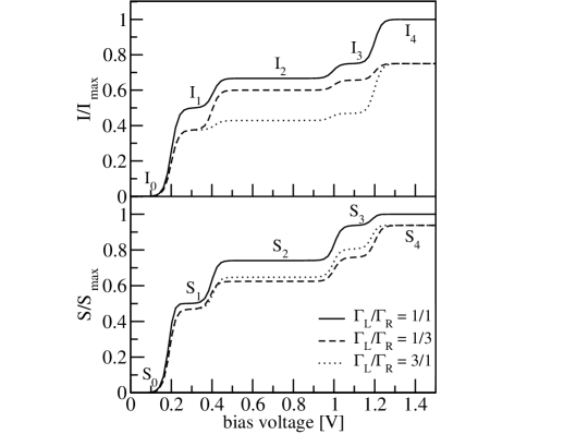
Figure 3: Current $I$ and shot noise $S$ vs. voltage for $T=100{\rm K}$, $\epsilon_{\downarrow}=0.1{\rm eV}$, $\epsilon_{\uparrow}=0.2{\rm eV}$, $U=0.4{\rm eV}$ and $\Gamma_{\rm L}/\Gamma_{\rm R}=$ 1/1 (solid line), 1/3 (dashed line), and 3/1 (dotted line). The height of the plateaus labeled by $i=0,..,4$ are given in Table 1. The curves are normalized to $I_{\rm max}=(e/\hbar)\Gamma/2$ and $S_{\rm max}=(e^{2}/\hbar)\Gamma/2$, respectively.

IV Results

In the following we discuss shot noise in the lowest- (first-) order perturbation theory in $\Gamma$. We consider transport through a single level and allow for a finite spin splitting. Such a spin splitting could be realized due to the Zeeman effect of an external magnetic field (for semiconductor quantum dots) or an intrinsic exchange field due to atoms with magnetic moments (for molecules). The molecule can acquire four possible states: the level being unoccupied, occupied with either spin $\uparrow$ or $\downarrow$, or doubly occupied. The molecular level is characterized by level energies $\epsilon_{\downarrow}$ and $\epsilon_{\uparrow}$, the Coulomb repulsion $U$, and the coupling strengths $\Gamma_{\rm L}$ and $\Gamma_{\rm R}$ to the electrodes. In addition, the electron distributions in the metal electrodes are governed by electrochemical potentials $\mu_{\rm L}$ and $\mu_{\rm R}$ and temperature $T$. We choose a symmetric bias voltage, such that $\mu_{\rm L}=eV/2$ and $\mu_{\rm R}=-eV/2$. In this simple model without real spatial extent, the voltage is dropped entirely at the electrode-molecule tunnel junctions, meaning that the energies of the molecular states are independent of the applied voltage even if the couplings are not symmetric. For asymmetric coupling this might not be entirely realistic. However, we do not wish to include a heuristic parameter to describe the possibly unequal drop of the bias. In a comparison to an actual experiment this could be easily amended. We also do not include an explicit gate voltage, as its effects are straightforward to anticipate.

In Fig. 3 we plot the current and the current noise for a special choice of system parameters as a function of transport voltage. For this figure we consider a set of energy parameters ($\epsilon_{\downarrow}=0.1{\rm eV}$,$\epsilon_{\uparrow}=0.2{\rm eV}$, $U=0.4{\rm eV}$) that is comparable to energies encountered in small molecules. A rescaling of energies by a factor 1/100 would be necessary to obtain energies of the order achievable in semiconductor quantum dots and by external magnetic fields. If the same scaling is applied to the couplings and the temperature, the figure would remain unchanged. This is a special feature of first-order transport.

Electron transport becomes possible when charge excitations on the molecule become energetically allowed. Generally, at low bias, transport is exponentially suppressed, unless a degeneracy of states with different net charge is present (this could be tailored by application of a gate voltage, which we do not consider here). Each time when one of the four excitation energies $\epsilon_{\downarrow}$, $\epsilon_{\uparrow}$, $\epsilon_{\downarrow}+U$, or $\epsilon_{\uparrow}+U$ enters the energy window defined by the electrochemical potentials of the electrodes, a transport channel opens. This gives rise to plateaus, separated by thermally broadened steps. Due to the symmetric application of the bias, the steps occur at voltages of twice the corresponding excitation energy. The plateau heights depend on the coupling parameters $\Gamma_{\rm L}$ and $\Gamma_{\rm R}$ only, i.e., they are independent of $U$ and $T$. The analytic expressions for current, noise, and Fano factor of these plateaus, which are labeled by $i=0,...,4$, are given in Table 1.

The curves in Fig. 3 are normalized to $I_{\rm max}=(e/\hbar)\Gamma/2$ and $S_{\rm max}=(e^{2}/\hbar)\Gamma/2$, respectively, which is reached in the large-bias limit for symmetric coupling $\Gamma_{\rm L}=\Gamma_{\rm R}$. For asymmetric coupling, the plateaus are reduced in height. In Fig. 3, we show the results for $3\Gamma_{\rm L}=\Gamma_{\rm R}$ (dashed lines) and $\Gamma_{\rm L}=3\Gamma_{\rm R}$ (dotted lines) together with the case of symmetric coupling. The symmetry of our setup implies that all plateau heights are invariant under simultaneous exchange of $\Gamma_{\rm L}$ with $\Gamma_{\rm R}$ and $\mu_{\rm L}$ with $\mu_{\rm R}$. However, the plateau height can change if only $\Gamma_{\rm L}$ and $\Gamma_{\rm R}$ are exchanged, or if only the bias voltage is reversed, as shown in our example for the two plateaus labeled by $2$ and $3$. This opens the possibility to access the asymmetry $\Gamma_{\rm L}/\Gamma_{\rm R}$ experimentally by reversing the bias voltage and comparing the plateau heights.

Table 1: Current, shot noise and Fano factor for the different plateaus in the current-voltage characteristic shown in Fig. 3. The plateau values depend only on the coupling parameters $\Gamma_{\rm L,R}$.

Figure 3 shows the result for one special choice of energy parameters and corresponding excitation energies. Nevertheless, Table 1 is complete in the sense that it contains all possible plateau values for any configuration of the excitation energies relative to the electrochemical potentials of the electrodes. The classification of the configurations and the algorithm to find the corresponding analytic expressions in Table 1 is given in Table 2. Without loss of generality we restrict ourselves to $U\geq 0$ and $\epsilon_{\uparrow}\geq\epsilon_{\downarrow}$. The different configurations are classified by specifying which excitation energies lie within the energy window defined by the chemical potentials $\mu_{\rm L},\mu_{\rm R}$. We find 13 different possibilities, as listed in Table 2. For each case, the index $i$ indicates the column where the corresponding analytic expressions for current, noise and Fano factor can be found in Table 1. The indices $2^{*}$ and $3^{*}$ refer to columns $2$ and $3$ but with $\Gamma_{\rm L}$ and $\Gamma_{\rm R}$ being exchanged.

Table 2: Classification of all possible configurations that are possible for $U\geq 0$ and $\epsilon_{\uparrow}\geq\epsilon_{\downarrow}$. A cross (x) or minus ($-$) indicates that the corresponding excitation energy lies within or outside the energy window defined by the electrochemical potentials $\mu_{\rm L}$ and $\mu_{\rm R}$, respectively. For each configuration, the analytic expression for current, noise and Fano factor can be found in Table 1 in column $i$. The indices $2^{*}$ and $3^{*}$ refer to column $2$ and $3$ with $\Gamma_{\rm L}$ and $\Gamma_{\rm R}$ being exchanged.

In order to illustrate the use of the table we sketch the situation $2a$ in Fig. 4, realized in Fig. 3 in the region between $0.4{\rm V}$ and $1{\rm V}$. In this situation transport through both spin states is present as the molecule gets charged/uncharged in the sequential tunneling events. Double occupancy is still out of reach, since the excitation energies $\epsilon_{\downarrow}+U$ and $\epsilon_{\uparrow}+U$ are outside the energy window opened by the applied voltage.

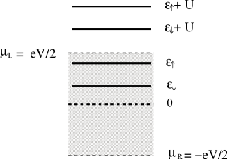
Figure 4: A sketch of the configuration $2a$ listed in Table 2. The excitation energies $\epsilon_{\downarrow}$ and $\epsilon_{\uparrow}$ lie in the energy window defined by the electrochemical potentials $\mu_{\rm L}$ and $\mu_{\rm R}$, and the energies $\epsilon_{\downarrow}+U$ and $\epsilon_{\uparrow}+U$ lie outside.

We now turn to the discussion of the Fano factor $F=S/2eI$. In Fig. 5 we show the Fano factor as a function of bias voltage for the same parameters as in Fig. 3. Again we show three curves with $\Gamma_{\rm L}/\Gamma_{\rm R}=1/1$ (solid line), $1/3$ (dashed line) and $3/1$ (dotted line). At small bias, $eV\ll k_{B}T$, the noise is dominated by thermal noise, described by the well-known hyperbolic cotangent behavior which leads to a divergence of the Fano factor.blanter ; loss The plateau for bias voltages below $0.2{\rm V}$ corresponds to the Coulomb-blockade regime, where transport is exponentially suppressed (case $0$ in Table 2). In the region between $0.2{\rm V}$ and $0.4{\rm V}$ (case $1a$) transport through only one spin state ($\downarrow$) is possible. The Fano factor $F_{1}$ for this case has been derived earlier in Ref. nazarov, . For very large bias (region $F_{4}$), all states of the molecular level are involved in transport, and the Fano factor $F_{4}$ is again identical to the well-known blanter formula for transport through a resonant level in the absence of Coulomb charging energy.

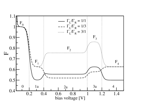
Figure 5: Fano factor vs. bias voltage for for the same parameters as in Fig. 3, namely $T=100{\rm K}$, $\epsilon_{\downarrow}=0.1{\rm eV}$,$\epsilon_{\uparrow}=0.2{\rm eV}$, $U=0.4{\rm eV}$, and $\Gamma_{\rm L}/\Gamma_{\rm R}=$ 1/1 (solid line), 1/3 (dashed line), and 3/1 (dotted line). The labels $0,1a,2a,3a,4$ refer to the cases listed in Table 2

For the regions in between, corresponding to the cases $2a$ and $3a$, the Fano factor is different. The expression for $F_{2}$ has been very recently derived in Ref. bagrets, , while $F_{3}$, corresponding to region $3a$, is, to the best of knowledge, a new result.

On similar grounds as for the current and the noise, we find that the expressions for the Fano factors $F_{2}$ and $F_{3}$ are not invariant under exchange of $\Gamma_{\rm L}$ and $\Gamma_{\rm R}$ alone, and also not invariant under reverse of the bias voltage alone. This is clearly seen in Fig. 5 in the very different plateau heights of the dotted and dashed curves, corresponding to exchange of $\Gamma_{\rm L}$ and $\Gamma_{\rm R}$. Furthermore, we see that all plateau heights lie between $1/2$ and $1$, and that the Fano factor, in general, is a nonmonotonic function of the bias voltage. We find that $F_{1}=F_{4}$ and $F_{3}\geq F_{2}$ always hold, whereas $F_{1}\geq F_{2}$ for $\Gamma_{\rm L}/\Gamma_{\rm R}\leq 1/\sqrt{2}$ and $F_{1}\geq F_{3}$ for $\Gamma_{\rm L}/\Gamma_{\rm R}\leq 1/2$ only.

As a consequence, the pattern of the plateau sequence, in particular the relative height of the plateaus $F_{2}$ and $F_{3}$ compared to $F_{1}=F_{4}$, indicates not only the presence of an interaction or charging energy, but also gives overcomplete information on the ratio $\Gamma_{\rm L}/\Gamma_{\rm R}$ of the coupling strengths. This could be used in experiments to determine these parameters in a consistent way. In an experiment observing more than one plateau, the overcompleteness would give narrow constraints (due to experimental uncertainty) on whether a single interacting level can explain the measured values. Of course, it is always possible to fit $n$ plateaus with $n$ noninteracting levels and different couplings per level, so an absolute decision on the presence of interactions is not possible without the additional application of a gate voltage. However, if a fit with an interacting level is feasible, the principle of parsimony should favor the model with fewer parameters.

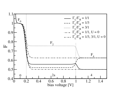
Figure 6: Fano factor vs. bias voltage in the absence of spin splitting. We chose $T=100{\rm K}$, $\epsilon_{\downarrow}=\epsilon_{\uparrow}=0.1{\rm eV}$, $U=0.4{\rm eV}$, and $\Gamma_{\rm L}/\Gamma_{\rm R}=$ 1/1 (solid line), 1/3 (dashed line), and 3/1 (dotted line). Also shown are the two cases for the corresponding noninteracting system ($U=0$).

In the absence of a spin splitting, $\epsilon_{\uparrow}=\epsilon_{\downarrow}$, the number of plateaus is reduced. An example for the Fano factor as a function of bias voltage is displayed in Fig. 6. The solid curve is for symmetric, and the dotted and dashed curves are for asymmetric coupling. Again, a nonmonotonic sequence of plateau heights, $F_{4}>F_{2}$, indicates the presence of Coulomb charging and $\Gamma_{\rm L}/\Gamma_{\rm R}<1/\sqrt{2}$. For comparison we remark that for both negligible spin splitting and zero charging energy ($U=0$), only the plateaus $F_{0}$ and $F_{4}$ appear, the plateau heights are invariant under reverse of bias, and no nonmonotonic behavior is seen, as also shown in Fig. 6.

Finally, we briefly comment on the steps connecting the plateaus of the Fano factor. In the present first-order approximation the steps are solely broadened by temperature. In addition, we observe that sometimes a peak in the Fano factor shows up. This happens, for example, at the step between $F_{1}$ and $F_{2}$ for $\Gamma_{\rm L}=\Gamma_{\rm R}$, as seen in Fig. 5. The peak height, $0.5625$, exceeds that of the adjacent plateaus, $0.5$ and $5/9$. These features can even appear in the regime of negligible Coulomb charging energy, as previously shown in Ref. haug, . However, we point out that the behavior at the steps is going to be strongly affected by second-order tunneling events, so-called cotunneling. For example, the current steps will show additional broadening due to the intrinsic linewidth $\Gamma$. On the other hand, the plateau values in regimes 1 - 4 will not be affected by second-order effects.

In summary, we presented a theory of transport through a molecule or quantum dot that allows for a systematic perturbation expansion of current and shot noise in the coupling strength between molecular orbital (dot level) and electrodes. We analyzed first-order transport in detail. In a complete overview, we derived analytic expressions for current, noise, and the Fano factor for all possible situations involving a single interacting level. In particular, we discussed how the sequence of Fano factor plateaus can provide information about the asymmetry ratio of the coupling strengths as well as the presence of Coulomb charging energy.

Acknowledgments. We enjoyed interesting and helpful discussions with A. Braggio, G. Johansson, H. Schoeller, H. Weber, and A. Zaikin, as well as financial support by the DFG via the Center for Functional Nanostructures and the Emmy-Noether program.

References

- (1) M. A. Reed, C. Zhou, C. J. Muller, T. P. Burgin, and J. M. Tour, Science 278, 252 (1997).
- (2) C. Kergueris, J. P. Bourgoin, S. Palacin, D. Esteve, C. Urbina, M. Magoga, and C. Joachim, Phys. Rev. B 59, 12505 (1999).
- (3) J. Reichert, R. Ochs, D. Beckmann, H. B. Weber, M. Mayor, and H. v. Löhneysen, Phys. Rev. Lett. 88, 176804 (2002).
- (4) M. Mayor, C. v. Hänisch, H. B. Weber, J. Reichert, and D. Beckmann, Angew. Chem. 114, 1228 (2002).
- (5) R. M. Metzger, B. Chen, U. Hopfner, M. V. Lakshmikantham, D. Vuillaume, T. Kawai, X. Wu, H. Tachibana, T. V. Hughes, H. Sakurai, J. W. Baldwin, C. Hosch, M. P. Cava, L. Brehmer, and G. J. Ashwell, J. Am. Chem. Soc. 119, 10455 (1997).
- (6) A. Vilan, A. Shanzer, and D. Cahen, Nature (London) 404, 166 (2000).
- (7) J. Chen and M. A. Reed, Chem. Phys. 281, 127 (2002).
- (8) V. A. Khlus, Zh. Eksp. Teor. Fiz. 93, 2179 (1987) [Sov. Phys. JETP 66, 1243 (1987) ].
- (9) G. B. Lesovik, Pis‘ma Zh. Eksp. Teor. Fiz. 49 (1989) 513 [JETP Lett. 49 (1989) 592].
- (10) Ya. M. Blanter and M. Büttiker, Phys. Rep. 336, 1 (2000).
- (11) M. H. Hettler, H. Schoeller, and W. Wenzel, Europhys. Lett. 57, 571 (2002); in Nano-Physics and Bio-Electronics: A New Odyssey, edited by T. Chakraborty, F. Peeters, and U. Sivan (Elsevier 2002).
- (12) M. H. Hettler, W. Wenzel, M. R. Wegewijs, and H. Schoeller, Phys. Rev. Lett. 90, 076805 (2003).
- (13) J. Park, A. N. Pasupathy, J. I. Goldsmith, C. Chang, Y. Yaish, J. R. Petta, M. Rinkoski, J. P. Sethna, H. D. Abruna, P. L. McEuen, and D. C. Ralph, Nature (London) 417, 722 (2002).
- (14) S. Hershfield, Phys. Rev. B 46, 7061 (1991).
- (15) Yu. V. Nazarov and J. J. R. Struben, Phys. Rev. B 53, 15466 (1996).
- (16) E. V. Sukhorukov, G. Burkard, and D. Loss, Phys. Rev. B 63, 125315 (2001).
- (17) D. A. Bagrets and Yu. V. Nazarov, Phys. Rev. B 67, 085316 (2003).
- (18) G. Kiesslich, A. Wacker, E. Schöll, A. Nauen, F. Hohls, and R. J. Haug, Phys. Status Solidi C 0, 1293 (2003).
- (19) J. König, H. Schoeller, and G. Schön, Phys. Rev. Lett. 76, 1715 (1996); J. König, J. Schmid, H. Schoeller, and G. Schön, Phys. Rev. B 54, 16820 (1996); H. Schoeller, in Mesoscopic Electron Transport, edited by L.L. Sohn, L.P. Kouwenhoven, and G. Schön (Kluwer, Dordrecht, 1997); J. König, Quantum Fluctuations in the Single-Electron Transistor (Shaker, Aachen, 1999).
- (20) A. N. Korotkov, Phys. Rev. B 49, 10381 (1993).