Vortex-unbinding and finite-size effects in Tl₂Ba₂CaCu₂O₈ thin films

Abstract

Current-voltage ($I$-$V$) characteristics of Tl₂Ba₂CaCu₂O₈ thin films in zero magnetic field are measured and analyzed with the conventional Kosterlitz-Thouless-Berezinskii (KTB) approach, dynamic scaling approach and finite-size scaling approach, respectively. It is found from these results that the $I$-$V$ relation is determined by the vortex-unbinding mechanism with the KTB dynamic critical exponent $z=2$. On the other hand, the evidence of finite-size effect is also found, which blurs the feature of a phase transition.

I Introduction

For two-dimensional (2D) systems in which the conventional long-range order is absent Mermin , the definition of topological order and Kosterlitz-Thouless-Berezinskii (KTB) transition Berezinskii ; Kosterlitz ; Kosterlitz1 has been proposed, with the latter characterized by a sudden change in the response of the system to the external perturbation. This type of transition was originally not considered to occur in superconductors Kosterlitz due to the dimensional restriction from the 2D penetration depth $\lambda_{\perp}$($\simeq\lambda^{2}/d$, with $\lambda$ the bulk penetration depth and $d$ the thickness of the film Pearl ), beyond which the logarithmic intra-pair binding interactions of vortices are saturated and free vortices will appear below the vortex-unbinding temperature. However, it was later argued that the KTB transition occurs in superconductors Halperin in a practical sense if $\lambda_{\perp}$ exceeds the system size, and this has been supported by experiments in dirty conventional superconductors Hebard with the enhanced $\lambda_{\perp}$.

For cuprate superconductors characterized by layered structure and high anisotropy, there have been early theoretical works about the KTB issue Rasolt . And the phase fluctuation has been argued to play an important role due to the low superfluid density Emery . This is supported by experiments including the high-frequency conductivity in underdoped Bi₂Sr₂CaCu₂O₈ (BSCCO) Corson , which revealed that the properties are dominated by the vortex-unbinding in the samples and that the short-time phase correlations persist above the superconducting transition temperature $T_{\rm c}$ and even up to the pseudogap temperature $T^{*}$, and the Nernst effect in underdoped La_2-xSr_xCuO₄ and Bi₂Sr_2-yLa_yCuO₆ Xu ; Wang reveals the existence of vortex-like excitation till the resolution limit (at temperatures 50-100 K above $T_{\rm c}$). The experiments probing the phase coherence have been considered much helpful in the research of KTB transition and high-$T_{\rm c}$ superconducting mechanism Millis .

As to the zero-field electrical transport characteristics, KTB theories have derived that Minnhagen ; Halperin , in the zero current ($I\rightarrow 0$) limit, the exponent $a$ of current-voltage ($I$-$V$) relation, $V=I^{a}$, will jump from 3 to 1 at the KTB transition temperature $T_{\rm KT}$, and the linear resistance $R_{\rm lin}$($\equiv\lim_{I\rightarrow 0}V/I$) is proportional to $\exp[-2\sqrt{b/(T/T_{\rm KT}-1)}]$, where $b$ is a non-universal constant. These features in the thermodynamic limit have been originally used in the determination of KTB transition, and is usually referred to as ‘conventional approach’.

Besides, the dynamic scaling approach proposed by Fisher, Fisher and Huse Fisher (FFH) has also been used in the study of KTB transition. In this ansatz, the data at finite currents are used in the scaling function, in which the dynamic critical exponent $z$, characterizing the relation between the relaxation time $\tau$ and the correlation length $\xi$ as $\tau=\xi^{z}$, equals 2 for a 2D superconductor in zero magnetic field. With the connection $a=1+z$ at the KTB transition temperature, this corresponds to $a=3$ in the conventional approach.

The experimental transport results of KTB transition in cuprates remain controversial. There have been reports of KTB transition in YBa₂Cu₃O_7-δ (YBCO) Matsuda , BSCCO Martin , and Tl₂Ba₂CaCu₂O₈ (TBCCO)Kim ; Wen systems. However, nanovolt-level current-voltage ($I$-$V$) measurements by Repaci et al.Repaci on single-unit-cell YBCO films show ohmic behavior far below the nominal KTB temperature. There are even results of $z\approx 6$, as given by Ammirata et al. Ammirata for the transport measurements of thin BSCCO crystal.

Holzer et al. Holzer simulated $I$-$V$ curves for 2D Josephson junction arrays, and argued that for the finite-size effect data, the scaling parameters $z$ and $T_{\rm KT}$ depends critically on the noise floor of the measuring system, and that the value $z\approx 6$ for a variety of 2D systems is related to the nature of data collection or the resolution of instrument, rather than characterizing some universality of physics.

Medvedyeva et al. Medvedyeva argued that the FFH dynamic scaling method is only appropriate for those phase transition with a finite correlation length $\xi$, thus is not compatible with a system undergoing a KTB transition with $\xi=\infty$ at temperatures below $T_{\rm KT}$. Instead they took the finite-size effect into account and argued that, for a 2D system with linear size $L$, the scaling behavior should be dependent on $L$ rather than $\xi$ at low temperatures for which $L<\xi(T)$, hence the electric field $E$ and the applied current density $J$ can be scaled as $E/JR_{\rm lin}=h(JLg_{L}(T))$ for small values of $J$, where $h(x)$ is the scaling function and $g_{L}(T)$ is the function that makes the $E/JR_{\rm lin}$-$JLg_{L}(T)$ curves collapse. Moreover, they performed the numerical simulations on 2D finite size ($L\times L$) systems with resistive-shunted-junction (RSJ) model, and re-analyzed the experimental data of Repaci et al.. Both numerical and experimental results suggest $z=2$. At the same time, an exponent $\alpha_{L}(T)$, which may depend on the system size $L$ and the temperature $T$, has been defined in the finite-size scaling scenario by $g_{L}(T)\equiv A_{L}R_{\rm lin}(T)^{-\alpha_{L}(T)}$, where $A_{L}$ is a universal constant for a given system with size $L$. Then it comes out that if $\alpha_{L}(T)$ is a constant ($\alpha_{L}(T)=\alpha$) for all the available data over a certain temperature region, the resistance will seem to vanish at the temperature for which $z(T)=1/\alpha$. For both 2D RSJ model and Repaci et al.’s data, it was found that $\alpha\approx 1/6$ in a limited temperature region by using the finite-size scaling approach, which amounts to $z\approx 6$. However, on the analogy of the results of 2D RSJ model, it was concluded that there is always a linear resistance at any temperatures for a finite-size system, and $\alpha\approx 1/6$ is only satisfied in a limited range, so the result $z\approx 6$ should not be considered as the symbol of a real transition.

In view of these controversies, we have carried out the research on Tl₂Ba₂CaCu₂O₈ thin films. The $R$-$T$ and $I$-$V$ characteristics was measured in zero magnetic field. This paper will begin the analyses with the conventional approach which focuses on the slope $a$ of the logarithmic $I$-$V$ curves in the $I\rightarrow 0$ limit, then the FFH dynamic scaling method will be used in analyzing the experimental data. Since the dynamic scaling method is argued to have some flexibility, the criteria of a real KTB transition proposed by Strachan et al.Strachan  have been used. Finally, we will follow the finite-size scaling procedures of Medvedyeva et al.. It is found that the experimental results are consistent with not only thermodynamic limit for which $z=2$, but also the exponent $\alpha\approx 1/2$, where $\alpha$ is the exponent defined by Medvedyeva et al.. On the other hand, the evidence of the finite-size effect is also found, suggesting a crossover rather than a real phase transition near the vortex-unbinding temperature $T_{\rm KT}$.

II Experiments

The Tl₂Ba₂CaCu₂O₈ films were prepared by a two-step procedure on (001) LaAlO₃ substrates. Details on the fabrication of the films have been published previously Yan . X-ray diffraction patterns (XRD) taken from the samples show that only (00$l$) peaks are observable, indicating a highly textured growth. The films with thickness of 150 nm were patterned lithographically into bridges with lateral dimensions of 33 $\mu$m $\times$ 500 $\mu$m.

$R$-$T$ and $I$-$V$ curves were measured using a standard four probe technique with a Keithley 182 nanovoltmeter and a Keithley 220 current source. A pulsed current is used for the resistance transition measurement, and the temperature of the sample holder was stabilized to better than 0.1 K during the measurement for each $I$-$V$ curve.

III Experimental results and analyses

The $R$-$T$ relation of the Tl₂Ba₂CaCu₂O₈ thin film in zero magnetic field is shown in Fig. 1. According to the logarithmic plot in the inset, there is $dT/d\ln R=0$ at a finite temperature, suggesting the existence of a zero-resistance state below it.

Figure 1: $R$-$T$ relation of a thin Tl₂Ba₂CaCu₂O₈ film in zero magnetic field. The inset displays $dT/d\ln R=0$ at a finite temperature, showing a zero-resistance transition.

The $I$-$V$ isotherms of the Tl₂Ba₂CaCu₂O₈ sample are plotted in Fig. 2. For our data, the determination of $a=3$ in the conventional approach is carried out at a common voltage with the current as small as possible, which is in the vicinity of $3\times 10^{-7}$ V. The broken line in Fig. 2 shows the condition $a=3$, therefore $T_{\rm KT}$ is determined as 103.8 K. It is interesting that the logarithmic $I$-$V$ curves show a positive curvature just above 103.8 K, indicating a finite linear resistivity above $T_{\rm KT}$.

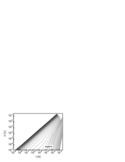
Figure 2: Logarithmic $I$-$V$ isotherms of the thin Tl₂Ba₂Ca- Cu₂O₈ film in zero magnetic field. The broken line indicates the slope $a=3$ at which the KTB transition occurs. The temperatures are from 95 K (the right side) to 116 K (the left side). The increasing step of the temperatures is 0.3 K at temperatures between 102 K and 109.5 K, otherwise it is 0.5 K. The transition temperature $T_{\rm KT}$ determined by this conventional approach is 103.8 K.

However, this conventional approach can be misleading Newrock in checking for $z=2$. For instance, it is difficult to determine the position of $a=3$, and the determination of $a(T)$ for a common voltage range (instead of a common current range) will introduce the effect of non-universal length scales. Therefore the dynamic scaling approach proposed by FFH Fisher is often used, in which the restriction of $I\rightarrow 0$ does not exist and data at finite currents are also used in the scaling. Thus we will apply this approach to our data.

For 2D superconductors, the dynamic scaling relation given by FFH is

$$V=I\xi^{-z}\chi_{\pm}(I\xi/T),$$ (1)

where $\chi_{+(-)}$ is the scaling function above (below) $T_{\rm KT}$, and $\xi$, with the original definition of correlation length in KTB theory, is not suitable for temperatures below $T_{\rm KT}$ because of its infinite value. It is then defined as the typical size of the vortex pairs below $T_{\rm KT}$ (for $\chi_{-}$)Newrock ; Ambegaokar . For convenience of scaling, Eq. (1) is often used as

$$\frac{I}{T}\bigg{(}\frac{I}{V}\bigg{)}^{1/z}=\epsilon_{\pm}(I\xi/T),$$ (2)

where $\epsilon_{\pm}(x)\equiv x/\chi_{\pm}^{1/z}(x)$. To proceed with the scaling in the form of Eq. (2), $\xi$ was assumed to be of KTB form $\xi_{\pm}(T)\propto\exp[\sqrt{b_{\pm}/|T/T_{\rm KT}-1|}]$, where the footnote $+(-)$ means at temperatures above (below) $T_{\rm KT}$, and $b$ is a non-universal constant. The FFH scaling results of the $I$-$V$ data of YBCO film measured by Repaci et al. Repaci suggest that $z=5.6\pm 0.3$ Medvedyeva . Following this approach, we show the scaling results of our $I$-$V$ data of Tl₂Ba₂CaCu₂O₈ film with $z=2$ and $z=5.6$ in Figure 3(a) and (b), respectively. The data are plotted in lines rather than points in order to expose any shortcomings in the scaling collapse as suggested by Holzer et al. Holzer . The upper (lower) branch of the plots corresponds to the temperatures below (above) $T_{\rm KT}$.

Figure 3: Dynamic scaling plots with scaling parameters (a) $z=2$ and (b) $z=5.6$. The correlation length $\xi$ is assumed to be of KTB form $\xi_{\pm}(T)\propto\exp[\sqrt{b_{\pm}/|T/T_{\rm KT}-1|}]$, where the footnote $+(-)$ means at temperatures above (below) $T_{\rm KT}$, and $b$ is a non-universal constant, thus $b_{+(-)}$ corresponds to the lower (upper) branch of the plots. The other scaling parameters are: (a) $T_{\rm KT}=103.8$ K, $b_{+}=0.21$, $b_{-}=3$; (b) $T_{\rm KT}=96$ K, $b_{+}=1.2$, $b_{-}=0.5$ (for the upper ($T<T_{\rm KT}$) branch the three short isotherms cannot get good collapse with any reasonable $b_{-}$ value).

For the high temperature ($T>T_{\rm KT}$) branch, the scaling collapse of data can be obtained with both $z=2$ and $z=5.6$. It shows that there is a crossover from $I^{1+1/z}/(TV^{1/z})\propto I\xi/T$ to $I^{1+1/z}/(TV^{1/z})=$ constant when $I$ increases. This corresponds to the crossover from $V\propto I$ to $V\propto I^{z+1}$ for each $I$-$V$ isotherm, which is shown obviously in Fig 2, especially for those isotherms near $T_{\rm KT}$. The crossover from linear to nonlinear $I$-$V$ relation is reflected in both Fig. 3(a) and (b), and Fig. 3(a) shows a much less nonlinear part than Fig. 3(b).

While for the low temperature ($T<T_{\rm KT}$) branch, a much better scaling collapse can be obtained with $z=2$ rather than $z=5.6$. As a matter of fact, for the $T<T_{\rm KT}$ branch of Fig. 3(b), a good scaling collapse is not available for $T_{\rm KT}$ and $b_{-}$ with any physically possible values. Moreover the $T_{\rm KT}$ for $z=5.6$ is much different from 103.8 K, the value obtained from the conventional approach.

Holzer et al.Holzer showed that for a finite-size system, the critical exponent $z$ derived from dynamic scaling becomes larger if the noise floor is lowered. This implies that the data with a fixed noise floor can be scaled with a $z$ value larger than the one characterizing a true phase transition, so there is some uncertainty if it is judged only from the dynamic scaling results Fig. 3(a) and (b).

Strachan et al. Strachan argued that the FFH scaling collapse alone is not a sufficient evidence of the phase transition, and proposed a criterion to determine the existence of a real KTB transition. That is, the logarithmic $I$-$V$ isotherms should show positive concavity above $T_{\rm KT}$, while show zero concavity at the same current level below the transition temperature. Furthermore, it can be distinguished from the finite-size-caused ohmic tail that, the current density $J_{\rm co}$, at which the $I$-$V$ relation crosses over from ohmic to non-ohmic behavior, should increase with temperature above $T_{\rm KT}$ for a true KTB transition, while decrease with temperature or be a constant for finite-size-caused unbinding.

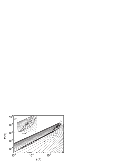
Figure 4: This Figure is used for two analysis procedures (so it suggests the similarity of the two): I. Strachan et al.’s criterion has been used where the crossover current $I_{\rm co}$ is determined by $V/IR_{\rm lin}=$ (a) 1.015, (b) 1.02, (c) 1.03, (d) 1.05. II. Direct determination of $z$ from the $I$-$V$ isotherms. The criteria are taken as $V/IR_{\rm lin}=$ (a) 1.015, (b) 1.02, (c) 1.03, (d) 1.05, and the determined $z$ value are (a) 1.67, (b) 2.19, (c) 3.48 and (d) 4.29, respectively. The temperatures at which the isotherms are dotted are from 105.9 to 110 K. Below 105.9 K there is no good $R_{\rm lin}$, and above 110 K the isotherms are too straight to reach the criteria value of $V/IR_{\rm lin}$. There is a distinct crossover for each $V_{\rm nl}$-$I_{\rm nl}$ curve at 107.1 K, which may be the temperature that $g_{L}(T)$ deviates obviously from $A_{L}R_{\rm lin}^{-\alpha}$ with $\alpha$ as a constant. The inset is an enlarged view of the fitted part.

This criterion has been used in Fig. 4, where the crossover current $I_{\rm co}$ is determined by $V/IR_{\rm lin}=$ 1.015, 1.02, 1.03 or 1.05 with $R_{\rm lin}$ the linear resistance. From 105.9 to 110 K, $I_{\rm co}$ increases with temperature. It is not available to see the temperatures between 103.8 and 105.9 K for the absence of the linear resistance, which may be caused by the limit of resolution.

At temperatures below 103.8 K, the logarithmic $I$-$V$ isotherms are straight (non-ohmic) at low currents, but tending toward ohmic at high currents, showing negative curvatures. This is similar to the $I$-$V$ simulations of Medvedyeva et al. Medvedyeva , which are interpreted Strachan as a possible result of the applicability of FFH scaling, the saturation of current-induced unbinding, or the reaching of bulk critical current of the sample, etc.

Medvedyeva et al. Medvedyeva also pointed out that dynamic scaling has much flexibility and can only be used in a system with the linear size $L\gg\xi$, so it is not compatible with a system undergoing a KTB transition because the correlation length $\xi=\infty$ at temperatures below $T_{\rm KT}$, and therefore only the scaling function $\chi_{+}$ above the KTB transition is justified. As to the low temperature phase, the finite size $L$ of the system serves as a cutoff in the length scale instead of $\xi$, and a finite-size scaling form

$$\frac{E}{JR_{\rm lin}}=h(JLg_{L}(T))$$ (3)

has been used for smaller values of $JLg_{L}(T)$, where $E$, $J$ and $L$ are the electric field, the applied current density and the linear size of the system, respectively, $R_{\rm lin}$ is the linear resistance, and $g_{L}(T)$ is a function of $T$ and $L$, which will have a finite value if $R_{\rm lin}$ is finite, or will diverge with a vanishing $R_{\rm lin}$. To proceed with their discussion about the finite-size scaling, $g_{L}(T)$ was defined as

$$g_{L}(T)=A_{L}R_{\rm lin}^{-\alpha_{L}(T)},$$ (4)

where $A_{L}$ is a universal constant which may depend on $L$. And it was claimed that if $\alpha_{L}(T)$ is a $T$-independent constant, Eq. (3) will be of the same form as dynamic scaling (an absolute correspondence requires $g_{L}(T)=A_{L}R_{\rm lin}^{-\alpha_{L}(T)}/T$, but here the unimportant denominator $T$ was neglected), in spite of the entirely incompatible theoretical ground. Furthermore, if all the available data are within the temperature region for which Eq. (4) is established, there will be a transition at $z(T)=1/\alpha$ which makes $g_{L}(T)\rightarrow\infty$ and hence corresponds to a vanishing resistance.

Since $V=LE$ and $I=LJ$ for a 2D $L\times L$ system Medvedyeva , Eq. (3) is equivalent to

$$\frac{V}{IR_{\rm lin}}=h(Ig_{L}(T)).$$ (5)

As mentioned by Medvedyeva et al., the slope $a(\equiv d\ln V/d\ln I)$ should be a constant $z(T)+1$ at small current for each isotherm below the KTB transition. For a finite-size system, however, it will cross over to 1 in the $I\rightarrow 0$ limit instead, resulting in the maxima in the plot. The maxima are controlled by variable $JL$ at low temperatures, while by variable $J\xi$ at higher temperatures above $T_{\rm KT}$. So there is also a crossover on the relevant current of each maximum, which occurs near the temperature at which $L\approx\xi$ and is not much higher than $T_{\rm KT}$. These two crossovers, on the value of the slope $a$ and on the position of the maxima, have been claimed as the symbols of finite-size effect. Moreover, by comparison of the RSJ simulation data with the conventional KTB theory, it was concluded that the slope values $a$ at the maxima are the same as the ones in the thermodynamic limit, so the maxima can be used to determine the KTB transition with the conventional criterion that $z=2$ or $a=3$.

Fig. 5 shows the slope $a\equiv d\ln V/d\ln I$ got from Fig. 2 versus $I$ in logarithmic scale. The data beyond the noise background have been removed. $T_{\rm KT}$ is 103.8 K, determined by the temperature of the $a$-$I$ curve which has the maximum of $a(=z+1)=3$. The result is consistent with that of previous approaches. Unlike the isotherms above $T_{\rm KT}$, there are no peaks appeared on the isotherms below $T_{\rm KT}$. When the temperature increases, the current at which the maxima appear decreases slightly at first, then increases rapidly (taking note of the logarithmic scale of $I$ in the plot), and the crossover occurs at the temperature of 105 K, which is somewhat higher than $T_{\rm KT}$. This agrees with the above picture of crossover on length scale ($L$-dominant to $\xi$-dominant) mentioned by Medvedyeva et al. from both simulation and the experimental results. A more detailed comparison with the work of Medvedyeva et al. suggests that in the $L$-dominant part of $a$-$I$ plot for Repaci’s YBCO data, the maxima appear at almost the same current, while for the 2D RSJ model, the maxima move toward the low current direction slightly with increasing temperature. Our data are more similar to the latter with more obvious decreasing.

Figure 5: The $I$-$V$ data plotted as $d\ln V/d\ln I$ against $I$ in logarithmic scale. The relevant temperatures decrease from the lower curves to higher ones. The broken line segments are used to connect the maxima which give estimates of $z(T)+1$. $T_{\rm KT}$ is determined by the temperature at which the maximum of the slope $d\ln V/d\ln I$ is 3. The result is consistent with the $T_{\rm KT}$ value got by the conventional approach that $T_{\rm KT}=103.8$ K. The crossover of the maxima occurs at 105 K, a temperature slightly higher than $T_{\rm KT}$.

The upturn of the curves at large currents may be caused by the heat effect hence it is not taken into account during the analyses.

Subsequently the question is whether the scaling given by Eq. (5) works. Fig. 6(a) shows the scaling collapse for our $I$-$V$ data. $V/IR_{\rm lin}$ is plotted against $Ig_{L}(T)$ and $g_{L}(T)$ is derived from the collapse of data. Because the linear resistance $R_{\rm lin}\equiv\lim_{I\rightarrow 0}d\ln V/d\ln I$ is required in the approach, which amounts to a requirement of a small current, the scaling is proceeded with the isotherms which can derive good linear resistance. The relevant temperatures are from 107.1 to 115.5 K which are above $T_{\rm KT}$ and in the regime where $\xi<L$. Nevertheless, the data show a good collapse for the finite-size scaling approach from a pragmatic point of view Medvedyeva . This connection of finite-size scaling with dynamic scaling implies the requirement that $\alpha_{L}(T)$ in Eq. (4) being a constant $\alpha$ is met.

For the temperatures lower than 107.1 K, including the region where the sample shows finite-size effect (at 105 K or temperatures lower, according to Fig. 5), the scaling collapses have not been obtained. This may be induced by the fact that the linear resistance $R_{\rm lin}$ and the voltage data at low enough currents, which are important elements in the finite-size scaling equation $V/IR_{\rm lin}=h(Ig_{L}(T))$, are not available.

To testify that $\alpha_{L}(T)$ is a constant and derive its value, the function of the form $A_{L}R_{\rm lin}^{-\alpha}/T$ should be used to fit $g_{L}(T)$ (in Eq. (4) Medvedyeva et al. neglected the unimportant denominator $T$ in $g_{L}(T)$, but here we keep it for better accuracy in fitting), where $R_{\rm lin}$ is the linear resistance determined from small current limit of the $I$-$V$ isotherms, $A_{L}$ and $\alpha$ are two fitting parameters. For convenience of fitting with smooth functions, we divide it into two steps. At first, the function $A^{\prime}_{L}\exp(\sqrt{b_{+}/(T/T_{\rm KT}-1)})/T$ is used for fitting, with $A^{\prime}_{L}$ and $b_{+}$ as two fitting parameters and regardless of the value of $\alpha$; secondly, linear fit the $\log R_{\rm lin}$-$\log[\exp(\sqrt{b_{+}/(T/T_{\rm KT}-1)})]$ relation and derive the slope, which corresponds to $-1/\alpha$. The above procedures come from the consideration that $R_{\rm lin}\propto\xi^{-z}$, $\xi\propto\exp(\sqrt{b_{+}/(T/T_{\rm KT}-1)})$ and $z=1/\alpha$ in the context of Medvedyeva et al.Medvedyeva . These two steps are shown in Fig. 6(b). The fitness shows that $g_{L}(T)$ is most likely to be represented by $\alpha=1/1.8$ ($z=1.8$), which is much closer to $z=2$ rather than $z=5.6$. At lower temperatures there is a visible deviation from the fit, which may be caused by finite-size effect.

Figure 6: (a) Determination of the existence of the scaling in the form of Eq. 5 for our $I$-$V$ data. $V/IR_{\rm lin}$ is plotted against $Ig_{L}(T)$, and $g_{L}(T)$ is derived from the collapse of data. The relevant temperatures are from 107.1 to 115.5 K, which corresponds to the $\xi<L$ regime above $T_{\rm KT}$. (b) The function $g_{L}(T)$ plotted versus $T$. The filled circles give the values of $g_{L}(T)$ determined from scaling collapse of $I$-$V$ data in (a). The fitting curve shows that $g_{L}(T)$ can be represented by $A^{\prime}_{L}\exp(\sqrt{b_{+}/(T/T_{\rm KT}-1)})/T$ with $A^{\prime}_{L}=23.4$ and $b_{+}=0.09$. The inset shows the linear resistance $R_{\rm lin}$ versus $\exp(\sqrt{b_{+}/(T/T_{\rm KT}-1)})$ plotted in $\log_{10}$-$\log_{10}$ scale. The slope of the fitting curve is $-1.8$, which suggest that $\alpha=1/1.8$ and $z=1.8$, which is much closer to the result $z=2$ rather than $z=5.6$.

According to Medvedyeva et al.Medvedyeva , the above results suggest that, if going down from a high temperature, a resistive transition will occur at some lower $T$ outside the region where Eq. (4) holds (with $\alpha=1/1.8$). That should correspond to the KTB transition ($z=2$).

Because the $I$-$V$ data can be scaled with Eq. (5), the linear part at small current corresponds to $V/IR_{\rm lin}=1$. And if $V/IR_{\rm lin}=c$ is taken as the criterion of the onset of the nonlinear relation on the $I$-$V$ isotherms, where $c$ is a constant, we will have

$$\frac{V_{\rm nl}}{I_{\rm nl}R_{\rm lin}}=h(I_{\rm nl}A_{L}R_{\rm lin}^{-\alpha_{L}(T)})=c,$$ (6)

where $h$ is the scaling function defined in Eq. (5), and ($I_{\rm nl}$, $V_{\rm nl}$) denotes the onset point on the $I$-$V$ isotherm, thus we have

$$\ln V_{\rm nl}=\Big{[}1+\frac{1}{\alpha_{L}(T)}\Big{]}\ln I_{\rm nl}+\Big{[}\ln c-\frac{1}{\alpha_{L}(T)}\ln\frac{c^{\prime}}{A_{L}}\Big{]},$$ (7)

where $c^{\prime}$ is the constant which satisfies $h(c^{\prime})=c$. Therefore if $\alpha$ is a constant within a temperature region, the logarithmic $V_{\rm nl}$-$I_{\rm nl}$ curve should be a straight line with the slope$=(1+1/\alpha)$ at these temperatures. So $\alpha$ can be determined directly from the slope of $V_{\rm nl}$-$I_{\rm nl}$ curve. This is exactly what Medvedyeva et al. did in Fig. 13 of Ref. Medvedyeva, .

Fig. 4 shows the $V_{\rm nl}$-$I_{\rm nl}$ curves with various criteria that $V/IR_{\rm lin}=c=1.015,1.02,1.03,1.05$, respectively. The relevant temperatures are from 105.9 to 110 K. There is a distinct crossover for each $V_{\rm nl}$-$I_{\rm nl}$ curve at 107.1 K, which is approximately the temperature that $g_{L}(T)$ begins to deviate obviously from $A_{L}R_{\rm lin}^{-\alpha}$ (see Fig. 6(b)) with a constant $\alpha$ value. As mentioned above, direct determination of $\alpha$ (or $z$) from the slope of $V_{\rm nl}$-$I_{\rm nl}$ curves only makes sense when $\alpha$ is a constant, thus the linear fit of $V_{\rm nl}$-$I_{\rm nl}$ curves should be carried out above 107.1 K, as shown by the dash lines. The results should be more reliable as the parameter $c$ decreases because the scaling function Eq. (5) is satisfied at currents not very high Medvedyeva . And the small $c$ results show that $z\approx 2$.

Fig. 7 shows the temperature dependence of linear resistance. The data obey Kosterlitz relation ($R_{\rm lin}\propto\exp(\sqrt{b_{+}/(T/T_{\rm KT}-1)})$) above 107.1 K, but deviate from the linear relation below 107.1 K. This may be interpreted as the crossover to finite-size effect. The directly measured $R$-$T$ data with a finite current drop more sharply than $R_{\rm lin}$ do.

Figure 7: Temperature dependence of the linear resistance. The dotted line is derived from the low current limit of Fig. 2, with the relevant temperatures from 104.7 to 116 K. The dashed line is from $R$-$T$ measurement taken at a finite current which is plotted in Fig. 1. The inset shows the logarithmic linear resistance $R_{\rm lin}$ versus $\sqrt{b_{+}/(T/T_{\rm KT}-1)}$, with a wider temperature range (105 to 116 K) than that of the inset of Fig. 6(b).

Since the above analyses suggest that the finite-size effect takes place in the $I$-$V$ data, the scaling collapse in Fig. 3 which is not so perfect can be attributed to that the data showing finite-size effect were scaled together with the data in the thermal dynamic limit by dynamic scaling method. So for the data at temperatures above $T_{\rm KT}$, if we remove those data showing finite-size effect and only consider the data at higher temperatures where $\xi_{+}\ll L$, the scaling collapse should be better. This is exhibited in Fig. 8 with the relevant scaling parameter $b_{+}$ changed. It shows that both $z=2$ and $z=5.6$ can give good collapse, which also suggest that some criterion is needed to eliminate the uncertainty.

Figure 8: Re-scaling of $I$-$V$ data with FFH method at higher temperatures where $\xi\ll L$ and all the data influenced by the finite-size effect are removed, including the data at temperatures slightly above that corresponding to $\xi\sim L$ (about 105 K), which still have some effect of finite size and are not collapsed well. The temperatures of the shown data are from 107.1 to 116 K, and the scaling parameters are: (a) $T_{\rm KT}=103.8$ K, $b_{+}=0.07$, $z=2$; (b) $T_{\rm KT}=96$ K, $b_{+}=0.12$, $z=5.6$.

A pure KTB transition, in the thermodynamic limit, requires Newrock $L\to\infty$ and $\lambda_{\perp}\gg L$. For the TBCCO sample with intrinsically high anisotropy, the estimated value of $\lambda_{\perp}(\sim\lambda^{2}/d)$ is about 60 $\mu$m with $\lambda=1500$ Å and $d=3.8$ Å, and the lateral sample size $L=33$ $\mu$m, thus the sample size $L$ is not much larger compared with the size of vortex pairs and $\lambda_{\perp}$ is not much greater than $L$, especially at zero temperature. Therefore the evidence of finite-size effect can be attributed to the finite cut-off length scale, which is $L$ rather than $\lambda_{\perp}$ for our data near the critical temperature.

IV Concluding Remarks

We have performed the conventional approach, FFH dynamic scaling approach and finite-size scaling approach proposed by Medvedyeva et al. on the data of thin Tl₂Ba₂CaCu₂O₈ films in zero magnetic field. The data in the small current limit together with those of finite values are studied. The results from all these methods are consistent with each other that the $I$-$V$ characteristics are dominated by the vortex-unbinding with the nominal transition temperature $T_{\rm KT}=103.8$ K, and the dynamic scaling exponent $z=2$ hence the $I$-$V$ exponent $a=3$ ($a\equiv d\ln V/d\ln I$).

Besides, the evidence of finite-size effect is also found, that the maxima of slope $a$ of logarithmic $I$-$V$ isotherms cross over from $L$-dependent to $\xi$-dependent with the crossover temperature at 105 K, slightly above $T_{\rm KT}$. The finite-size-caused free vortices will lead to the absence of a phase transition in a strict sense, and will turn the phase transition into a crossover behavior Newrock . However, the finite-size effect in our experiments is not so remarkable that, even at the voltage measuring limit the $I$-$V$ isotherms are not showing a linear resistivity. Medvedyeva et al. Medvedyeva gave an explanation for the $I$-$V$ data of Repaci et al. which show $z\approx 6$. The transition has been called a “ghost” transition because it is only a finite-size effect and does not occur in the thermodynamic ($L\gg\xi$) limit. In our case, however, the transition at the temperature below $\alpha=1/1.8$ expected by the finite-size scaling should correspond to the vortex-unbinding transition with $z=2$, behaving more likely as the thermodynamic limit rather than a “ghost” transition. This can be interpreted by the high experimental temperature near $T_{\rm c}$ so that the size of our sample is not in the finite-size limit as that in the simulation work of Medvedyeva et al., therefore it is sufficient to bring a finite-size effect in the KTB transition but does not markedly change the $z=2$ result.

- (1) N. D. Mermin, Phys. Rev. 176, 250 (1968). N. D. Mermin and H. Wagner, Phys. Rev. Lett. 22, 1133 (1966). P. C. Hohenberg, Phys. Rev. 158, 383 (1967).
- (2) V. L. Berezinskii, Sov. Phys. JETP 34, 610 (1972).
- (3) J. M. Kosterlitz and D. J. Thouless, J. Phys. C 6, 1181 (1973).
- (4) J. M. Kosterlitz and D. R. Nelson, Phys. Rev. Lett. 39, 1201 (1977).
- (5) J. Pearl, Appl. Phys. Lett. 5, 65 (1964).
- (6) B. I. Halperin and D. R. Nelson, J. Low Temp. Phys. 36, 599 (1979).
- (7) A. F. Hebard and A. T. Fiory, Phys. Rev. Lett. 50, 1603 (1983). P. A. Bancel and K. E. Gray, Phys. Rev. Lett. 46, 148 (1981).
- (8) M. Rasolt, T. Edis, and Z. Tesanovic, Phys. Rev. Lett. 66, 2927 (1991).
- (9) V. J. Emery and S. A. Kivelson, Nature 374, 434 (1995).
- (10) J. Corson, R. Mallozzi, J. Orenstein, J. N. Eckstein, and I. Bozovic, Nature 398, 221 (1999).
- (11) Z. A. Xu, N. P. Ong, Y. Wang, T. Kakeshita, and S. Uchida, Nature 406, 486 (2000).
- (12) Y. Wang, Z. A. Xu, T. Kakeshita, S. Uchida, S. Ono, Yoichi Ando, and N. P. Ong, Phys. Rev. B 64, 224519 (2001).
- (13) A. J. Millis, Nature 398, 193 (1999).
- (14) P. Minnhagen, Rev. Mod. Phys. 59, 1001 (1987).
- (15) D. S. Fisher, M. P. A. Fisher, and D. A. Huse, Phys. Rev. B 43, 130 (1991).
- (16) Y. Matsuda and S. Komiyama, Phys. Rev. B 48, 10498 (1993).
- (17) S. Martin, A. T. Fiory, R. M. Fleming, G. P. Espinosa, and A. S. Cooper, Phys. Rev. Lett. 62, 677 (1989).
- (18) D. H. Kim, A. M. Goldman, J. H. Kang, and R. T. Kampwirth, Phys. Rev. B 40, 8834 (1989).
- (19) H. H. Wen, P. Ziemann, H. A. Radovan and S. L. Yan, Europhys. Lett. 42(3), 319 (1998).
- (20) J. M. Repaci, C. Kwon, Q. Li, X. Jiang, T. Venkatessan, R. E. Glover, C. J. Lobb, and R. S. Newrock, Phys. Rev. B 54, R9674 (1996).
- (21) S. M. Ammirata, M. Friesen, S. W. Pierson, LeRoy A. Gorham, Jeffrey C. Hunnicutt, M. L. Trawick, and C. D. Keener, Physica C 313, 225 (1999).
- (22) J. Holzer, R. S. Newrock, C. J. Lobb, T. Aouaroun, and S. T. Herbert, Phys. Rev. B 63, 184508 (2001).
- (23) K. Medvedyeva, B. J. Kim, and P. Minnhagen, Phys. Rev. B 62, 14531 (2000).
- (24) D. R. Strachan, C. J. Lobb, and R. S. Newrock, unpublished.
- (25) S. L. Yan, L. Fang, Q. X. Song, J. Yan, Y. P. Zhu, J. H. Chen, and S. B. Zhang, Appl. Phys. Lett. 63, 1845 (1993).
- (26) R. S. Newrock, C. J. Lobb, U. Geigenmller, and M. Octavio, Solid Stat. Phys. 54, 263 (2000).
- (27) V. U. Ambegaokar, B. I. Halperin, D. R. Nelson, and E. D. Siggia, Phys. Rev. Lett. 40, 783 (1978). V. U. Ambegaokar, B. I. Halperin, D. R. Nelson, and E. D. Siggia, Phys. Rev. B 21, 1806 (1980).