Current Characteristics of the Single-Electron Transistor at the Degeneracy Point

Abstract

The linear and nonlinear transport properties of the single-electron transistor at the degeneracy point are investigated for the case of weak single-mode tunnel junctions. Two opposing scenarios are considered, distinguished by whether or not electrons can propagate coherently between the two tunnel junctions. Each of these two scenarios corresponds to the realization of a different multichannel Kondo effect — the two-channel Kondo effect in the case where coherent propagation is allowed, and the four-channel Kondo effect in the absence of coherent propagation. A detailed analysis of the linear and nonlinear conductance is presented for each of these scenarios, within a generalized noncrossing approximation for the nonequilibrium multichannel Kondo Hamiltonian. A zero-bias anomaly is shown to develop with decreasing temperature, characterized by the anomalous power laws of the multichannel Kondo effect. A scaling function of the differential conductance with $V/T$ ($V$ being the applied voltage bias, $T$ the temperature) is proposed as a distinctive experimental signature for each of these two scenarios. In the absence of coherent propagation between the leads, and for asymmetric couplings to the two leads, a crossover from four-channel to two-channel behavior is manifested in a vanishing zero-temperature conductance, and in a nonmonotonic voltage dependence of the differential conductance for small asymmetries.

]

I Introduction

The single-electron transistor — a small metallic or semiconducting quantum box connected to two separate leads — is among the basic elements of mesoscopic devices. Due to the finite energy barrier for charging the box with a single electron, the so-called Coulomb blockade, [1, 2] charge inside the box is nearly quantized at low temperatures for weak tunneling between the box and the leads. As a result, transport through the box is strongly suppressed unless the two lowest lying charge configurations in the box are tuned to be degenerate. As a function of gate voltage, the conductance thus shows a sequence of narrow peaks, each corresponding to the crossing of the ground state from $n$ to $n+1$ excess electrons inside the box.

At the degeneracy points, the system is subject to strong charge fluctuations. The corresponding low-energy physics is governed by the non-Fermi-liquid fixed point of the multichannel Kondo effect, [3, 4, 5] where the two degenerate charge configurations in the box play the role of the impurity spin. Which multichannel Kondo effect is realized depends on microscopic details such as the number of transverse modes in the junctions, and the nature of electron transport inside the box. Two opposing scenarios were considered to date for the single-electron transistor, distinguished by whether or not electrons can propagate coherently between the two tunnel junctions. Focusing on wide tunnel junctions, König et al. [6] considered the case where electrons can propagate coherently between the two leads (see also Refs. [7] and [8]). Extending the work Grabert [9] to nonequilibrium transport, these authors analyzed in detail all second-order contributions to the current in the dimensionless tunneling conductance, obtaining good agreement with experiment. [10] However, based on perturbation theory, this approach breaks down near the degeneracy points, where transport is governed at low temperature by the strong electronic correlations of the multichannel Kondo effect.

An alternative scenario was considered by Furusaki and Matveev, [11] and later by Zaránd et al. [12] and Le Hur and Seelig. [13] Noting that elastic cotunneling is strongly suppressed at temperatures above the level spacing, [14] these authors omitted altogether coherent electron transport between the leads, by coupling each lead to independent conduction-electron modes within the box. For symmetric single-mode junctions, the resulting low-temperature physics is governed at the degeneracy point by the four-channel Kondo effect, [11] in contrast to the two-channel Kondo effect that takes place when electrons can propagate coherently between the leads. Any asymmetry in the coupling to the two leads drives the system away from the four-channel fixed point to a two-channel fixed point, where one lead is decoupled from the box. Consequently, the zero-temperature conductance vanishes, as shown by Furusaki and Matveev in the limit of both a large asymmetry and strong tunneling to one lead [11] (i.e., a nearly open tunneling mode). A quantitative description of the temperature and asymmetry dependence of the conductance in this case remains lacking.

Despite considerable efforts, [6, 7, 8, 11, 12, 13] the understanding of the low-temperature transport at the degeneracy points is far from complete for either scenario. For weak single-mode tunnel junctions, there is no quantitative theory for the temperature dependence of the conductance in the Kondo regime, while the nonequilibrium differential conductance is practically unexplored in this regime for either scenario. [15] The goal of this paper is to provide a detailed analysis of the linear and nonlinear transport at resonance, for weak single-mode tunnel junctions. Both scenarios where electrons either can or cannot propagate coherently between the two junctions are considered. Our aim is to provide a host of signatures that can be used to experimentally discern the two pictures, and to detect which multichannel Kondo effect is realized in actual systems. [16]

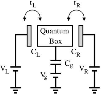
FIG. 1.: Schematic description of the physical system. A quantum box is coupled capacitively to a gate, and connected by weak tunneling ($t_{L}$ and $t_{R}$) to two metallic leads: a left lead and right lead. The charge inside the box is controlled by varying the gate voltage $V_{g}$, which fixes the electrostatic potential within the box. A drain-source voltage bias $V=V_{R}-V_{L}$ is applied across the transistor, which drives a current through the device.

To this end, we employ the noncrossing approximation [17] (NCA). The NCA is a self-consistent perturbation theory about the atomic limit. Originally designed to study dilute magnetic alloys, this approach was successfully applied to the out-of-equilibrium Kondo effect both for the single-channel [18, 19, 20] and two-channel [21] Anderson impurity model. Recently, the NCA was generalized to the multichannel Kondo spin Hamiltonian with arbitrary spin-exchange and potential-scattering couplings. [22] Similar to the NCA formulation of the multichannel Anderson model, [23] the Kondo-NCA (KNCA) correctly describes the low-energy physics of the multichannel Kondo model, reproducing the exact non-Fermi-liquid power laws and logarithms of the multichannel Kondo effect. This should be contrasted with the single-channel case, where the NCA (and KNCA) fails to describe the Fermi-liquid fixed point. [17] Here we extend the KNCA approach to the nonequilibrium case, and apply it to the single-electron transistor.

Using the KNCA, we find that a zero-bias anomaly develops in the current characteristics of the single-electron transistor, featuring the anomalous power laws of the corresponding multichannel Kondo effect. The latter power laws are manifest in the temperature and voltage dependences of the low-temperature, low-bias differential conductance. Similar to the case of two-channel Kondo scattering off nonmagnetic two-level tunneling systems, [21, 24] these power laws are best revealed in a scaling plot of the differential conductance versus $eV/k_{B}T$, with $V$ being the applied voltage bias. Such scaling plots are proposed as a distinct experimental signature of the appropriate multichannel Kondo effect. In the absence of electron propagation between the two leads, a crossover from four-channel to two-channel behavior is found in the differential conductance for asymmetric couplings, in accordance with the picture of Furusaki and Matveev. [11]

The remainder of the paper is organized as follows. In sec. II we present the single-electron transistor, and discuss the two alternative models under consideration. The nonequilibrium KNCA is then formulated in sec. III, followed by the derivation of the current in sec. IV. Our results for the linear and nonlinear transport are presented in sec. V, and discuss in sec. VI.

II The single-electron transistor

A Basic model

The physical system under consideration is shown schematically in Fig. 1. A metallic island, or quantum box, is connected by narrow point contacts to two separate leads, a left lead ($L$) and a right lead ($R$). A drain-source voltage bias is applied across the device, which sets a chemical-potential difference between the leads: $\mu_{L}-\mu_{R}=eV$. Here $-e$ is the electron charge. Modeling each lead by $N$ noninteracting one-dimensional conduction modes, the Hamiltonian of the two independent leads reads

$${\cal H}_{leads}=\sum_{\alpha=L,R}\sum_{n=1}^{N}\sum_{k,\sigma}(\epsilon_{\alpha kn}+\mu_{\alpha})c^{\dagger}_{\alpha kn\sigma}c_{\alpha kn\sigma},$$ (1)

where $c^{\dagger}_{\alpha kn\sigma}$ creates a conduction electron with wave number $k$ and spin projection $\sigma$ in the $n$th mode of lead $\alpha$, and $\epsilon_{\alpha kn}$ are the corresponding single-particle energies, measured relative to the chemical potential on that lead.

For the quantum box, one has to consider also its charging energy. Setting the Fermi energy of the box as our reference energy for the single-particle levels inside the box, the excess number of electrons on the metallic island is described by the operator

$$\hat{N}_{B}=\sum_{m=1}^{M}\sum_{q,\sigma}\left[c^{\dagger}_{Bqm\sigma}c_{Bqm\sigma}-\theta(-\epsilon_{Bqm})\right].$$ (2)

Here, similar to our notation for the leads, $c^{\dagger}_{Bqm\sigma}$ creates an electron with wave number $q$ and spin projection $\sigma$ in the $m$th mode of the box ($M$ independent conductance modes are taken within the box), and $\epsilon_{Bqm}$ are the corresponding single-particle levels. The latter levels are assumed to be sufficiently dense such that a continuum-limit description can be used. The Hamiltonian of the isolated box is thus given by

$${\cal H}_{box}=\sum_{m=1}^{M}\sum_{q,\sigma}\epsilon_{Bqm}c^{\dagger}_{Bqm\sigma}c_{Bqm\sigma}+E_{C}\left(\hat{N}_{B}-N_{C}\right)^{2},$$ (3)

where $E_{C}$ is the charging energy of the box, and $N_{C}$ is the classical number of excess electrons inside the box. These two quantities are related to the capacitances of the gate and of the left and right junctions through $E_{C}=e^{2}/2(C_{g}+C_{L}+C_{R})$ and $N_{C}=(C_{g}V_{g}+C_{L}V_{L}+C_{R}V_{R})/e$, where $V_{g}$, $V_{L}$, and $V_{R}$ are the voltages applied to the gate and to the left and right leads, respectively (see Fig. 1).

The quantum box is coupled to the leads by weak tunneling, described by the tunneling Hamiltonian

$${\cal H}_{tunnel}=\sum_{\alpha=L,R}\sum_{n,m}\sum_{k,q,\sigma}t^{\alpha}_{nm}\left\{c^{\dagger}_{\alpha kn\sigma}c_{Bqm\sigma}+{\rm H.c.}\right\}.$$ (4)

For simplicity, both the $k$ and $q$ dependences of the tunneling matrix elements $t^{L}_{nm}$ and $t^{R}_{nm}$ have been neglected in Eq. (4). The full Hamiltonian of the system reads ${\cal H}={\cal H}_{leads}+{\cal H}_{box}+{\cal H}_{tunnel}$.

B Mapping onto the multichannel Kondo problem

Our objective is a detailed quantitative description of the linear and nonlinear transport at resonance, when two neighboring charge configurations are degenerate within the box. To this end, let us focus on the vicinity of a particular degeneracy point, $N_{C}=n+\frac{1}{2}$ with $n$ an integer, separating the $\hat{N}_{B}=n$ and $\hat{N}_{B}=n+1$ charge configurations.

As emphasized by Matveev, [3, 4] the low-temperature, low-bias physics is governed at resonance by the intermediate-coupling fixed point of the multichannel Kondo effect. To formulate the connection between the two problems, we proceed along the lines laid out by Matveev. [3] Labeling the deviation from the degeneracy point by $\delta N=N_{C}-n-\frac{1}{2}$, we concentrate on $|\delta N|\ll 1$ and $e|V|,k_{B}T\ll e^{2}/C_{B}$, such that all charge configurations in the box other than $\hat{N}_{B}=n$ and $\hat{N}_{B}=n+1$ are energetically inaccessible. One can formally remove all higher energy charge configurations in the box by means of two projection operators, $P_{n}$ and $P_{n+1}$, which project onto the $\hat{N}_{B}=n$ and $\hat{N}_{B}=n+1$ subspaces, respectively. Alternatively, one can carry out the projection onto the low-energy subspace by introducing a spin-$\frac{1}{2}$ isospin operator $\vec{S}$, and identifying

$$P_{n+1}-P_{n} \longleftrightarrow 2S_{z},$$ (5)

$$P_{n}c_{Bqm\sigma}P_{n+1} \longleftrightarrow c_{Bqm\sigma}S^{-},$$ (6)

$$P_{n+1}c^{\dagger}_{Bqm\sigma}P_{n} \longleftrightarrow c^{\dagger}_{Bqm\sigma}S^{+}.$$ (7)

Omitting an $E_{C}$-dependent reference energy, the resulting low-energy Hamiltonian reads

$${\cal H}_{\rm eff} = \sum_{\alpha=L,R}\sum_{k,n,\sigma}(\epsilon_{\alpha kn}+\mu_{\alpha})c^{\dagger}_{\alpha kn\sigma}c_{\alpha kn\sigma}$$ (8)

$$+ \sum_{q,m,\sigma}\epsilon_{Bqm}c^{\dagger}_{Bqm\sigma}c_{Bqm\sigma}-2E_{C}\delta NS_{z}$$ (9)

$$+ \sum_{\alpha=L,R}\sum_{k,q,n,m,\sigma}\left\{t^{\alpha}_{nm}c^{\dagger}_{\alpha kn\sigma}c_{Bqm\sigma}S^{-}+{\rm H.c.}\right\}.$$ (10)

Strictly speaking, Eqs. (5)–(10) are subject to the constraint $\hat{N}_{B}-S_{z}=n+1/2$, reflecting the fact that the isospin $\vec{S}$ and the conduction-electron operators $c^{\dagger}_{Bqm\sigma}$ are not independent degrees of freedom. However, since the isospin dynamics in the Hamiltonian of Eq. (10) is not sensitive to the precise number of conduction electrons inside the quantum box, this constraint can be conveniently relaxed. We therefore regard hereafter the isospin $\vec{S}$ and the $c^{\dagger}_{Bqm\sigma}$ operators as independent.

The Hamiltonian of Eq. (10) has the form of a planner multichannel Kondo Hamiltonian. Here $h=2E_{C}\delta N$ plays the role of a magnetic field, while the equivalence of the two spin orientations guarantees the existence of at least two identical conduction-electron channels. The total number of independent conduction-electron channels depends, however, on the microscopic details of the $t_{nm}^{\alpha}$ tunneling matrix elements. In this paper we consider two particular scenarios, corresponding to the two- and four-channel planner Kondo Hamiltonian.

C Coherent propagation versus no coherent propagation between the two junctions

For sufficiently narrow point contacts, only a single mode weakly couples each lead to the quantum box. Focusing on this case, we consider two different scenarios: one by which both leads couple to the same single mode within the box, and the other whereby each lead is coupled to a different mode within the box.

The former scenario is just a single-mode version of the model of König et al., [6] whereby electrons can propagate coherently between the two leads. Its corresponding low-energy effective Hamiltonian is obtained by setting $N=M=1$ in Eqs. (1)–(4), thus omitting the mode indices $n$ and $m$. The resulting Hamiltonian takes the form

$${\cal H}_{\rm eff} = \sum_{\alpha=L,R}\sum_{k,\sigma}(\epsilon_{\alpha k}+\mu_{\alpha})c^{\dagger}_{\alpha k\sigma}c_{\alpha k\sigma}+\sum_{q,\sigma}\epsilon_{Bq}c^{\dagger}_{Bq\sigma}c_{Bq\sigma}$$ (11)

$$+ \sum_{\alpha=L,R}\sum_{k,q,\sigma}t_{\alpha}\left\{c^{\dagger}_{\alpha k\sigma}c_{Bq\sigma}S^{-}+{\rm H.c.}\right\}-hS_{z},$$ (12)

where $t^{L}_{nm}\to t_{L}$ and $t^{R}_{nm}\to t_{R}$ (both taken to be real) are the tunneling matrix elements for the left and right junctions, respectively.

The second scenario is a straightforward adaptation to weak single-mode tunnel junctions of the model introduced by Furusaki and Matveev, [11] and later used by Zaránd et al. [12] and by Le Hur and Seelig. [13] In this model, electron propagation between the two leads is excluded from the outset, accounting thereby for the strong suppression of elastic cotunneling at temperatures above the level spacing. [14] The corresponding low-energy effective Hamiltonian is obtained from Eqs. (1)–(4) by setting $N=1$ and $M=2$, and taking $t^{L}_{1m}\to t_{L}\delta_{m,1}$ and $t^{R}_{1m}\to t_{R}\delta_{m,2}$. Converting for convenience from the channel labels $m=1$ and $m=2$ within the box to $\alpha=L$ and $\alpha=R$, respectively, the resulting Hamiltonian is given by

$${\cal H}_{\rm eff} = \sum_{\alpha=L,R}\sum_{k,\sigma}(\epsilon_{\alpha k}+\mu_{\alpha})c^{\dagger}_{\alpha k\sigma}c_{\alpha k\sigma}$$ (13)

$$+ \sum_{\alpha=L,R}\sum_{q,\sigma}\epsilon_{Bq\alpha}c^{\dagger}_{Bq\alpha\sigma}c_{Bq\alpha\sigma}-hS_{z}$$ (14)

$$+ \sum_{\alpha=L,R}\sum_{k,q,\sigma}t_{\alpha}\left\{c^{\dagger}_{\alpha k\sigma}c_{Bq\alpha\sigma}S^{-}+{\rm H.c.}\right\}.$$ (15)

As in Eq. (12), the effective magnetic field $h$ is equal to $2E_{C}\delta N$.

1 Coherent propagation between the leads

The Hamiltonian of Eq. (12) is equivalent in equilibrium to the planner two-channel Kondo Hamiltonian in an applied magnetic field. This is best seen by first converting to a constant-energy-shell representation of the conduction-electron creation and annihilation operators in each of the two leads and the quantum box, and then constructing generalized “bonding” and “anti-bonding” combinations of the two leads. Upon doing so the “anti-bonding” band decouples from the isospin $\vec{S}$, while the “bonding” band plays the role of the single lead in Matveev’s original mapping onto the planner two-channel Kondo Hamiltonian. [3] At the degeneracy point, the capacitance of the single-electron transistor diverges logarithmically with decreasing temperature according to $C\propto(1/T_{K})\log(T_{K}/T)$, where $T_{K}$ is the two-channel Kondo temperature: [25]

$$k_{B}T_{K}=\left(D\sqrt{g_{L}+g_{R}}\right)\exp\left[-\frac{\pi}{4\sqrt{g_{L}+g_{R}}}\right].$$ (16)

Here $D\sim 2E_{C}$ is the effective conduction-electron bandwidth,

$$g_{\alpha}=\rho_{\alpha}(0)\rho_{B}(0)t_{\alpha}^{2}$$ (17)

($\alpha=L,R$) are the dimensionless tunneling conductances for the left and right junctions, and

$$\rho_{\gamma}(\epsilon)=\sum_{k}\delta(\epsilon-\epsilon_{\gamma k})$$ (18)

are the underlying density of states ($\gamma=L,R$, or $B$). Throughout this paper we use the notation by which the argument of $\rho_{\gamma}(\epsilon)$ is measured relative to the corresponding chemical potential, i.e., $\mu_{L}$ and $\mu_{R}$ for $\gamma=L$ and $R$, respectively, and $\mu_{B}=0$ for $\gamma=B$.

Away from equilibrium, it is still possible to construct “bonding” and “anti-bonding” combinations of the left and right leads, yet one can no longer dismiss the “anti-bonding” degrees of freedom as irrelevant. While the latter degrees of freedom remain decoupled from the isospin $\vec{S}$ on the level of the Hamiltonian, they do couple to $\vec{S}$ through the effective density matrix, which assigns different chemical potentials to the right and left leads. Hence both the “bonding” and “anti-bonding” combinations must be retained when computing the current for a finite bias.

2 No coherent propagation between the leads

Contrary to the Hamiltonian of Eq. (12), the Hamiltonian of Eq. (15) corresponds in equilibrium to the planner four-channel Kondo Hamiltonian with channel anisotropy. Specifically, there are two distinct pairs of equivalent channels, one pair for each tunnel junction. A channel-isotropic four-channel Kondo Hamiltonian is recovered only for equal tunneling conductances for the left and right junctions, $g_{L}=g_{R}$. The latter conductances are given by

$$g_{\alpha}=\rho_{\alpha}(0)\rho_{B\alpha}(0)t_{\alpha}^{2}$$ (19)

($\alpha=L,R$), which differ from the expressions of Eq. (17) only in the separate density of states for the left and right modes within the quantum box:

$$\rho_{B\alpha}(\epsilon)=\sum_{k}\delta(\epsilon-\epsilon_{Bk\alpha}).$$ (20)

For $g_{L}=g_{R}=g$, the low-energy physics of the transistor is governed by the non-Fermi-liquid fixed point of the four-channel Kondo effect. The corresponding Kondo temperature is given by [26]

$$k_{B}T_{K}=(Dg)\exp\left[-\frac{\pi}{4\sqrt{g}}\right],$$ (21)

where $D\sim 2E_{C}$. Note that the exponent of Eq. (21) differs by a factor of $\sqrt{2}$ from that of Eq. (16) under the same condition that $g_{L}=g_{R}=g$. Any asymmetry in the left and right tunneling conductances, $g_{L}\neq g_{R}$, drives the system to a two-channel fixed point with one of the leads effectively decoupled from the box.

III Noncrossing approximation

To obtain a reliable quantitative theory for the low-temperature transport at resonance for each of the models of Eqs. (12) and (15), we resort to a recent adaptation of the noncrossing approximation (NCA) to the Kondo spin Hamiltonian with arbitrary spin-exchange and potential-scattering couplings. [22] In this section, we formulate the Kondo-NCA (KNCA) for each of the models of Eqs. (12) and (15), generalizing the KNCA to nonequilibrium.

A Slave-fermion representation

To handle the isospin ${\vec{S}}$, which we refer to hereafter as the impurity spin, we employ Abrikosov’s slave-fermion representation. [27] In this representation, one assigns a pseudo fermion to each impurity spin state according to

$$f_{+}^{\dagger}\left|0\right\rangle \longleftrightarrow \left|S_{z}=+1/2\right\rangle,$$ (22)

$$f_{-}^{\dagger}\left|0\right\rangle \longleftrightarrow |S_{z}=-1/2\rangle.$$ (23)

This assignment corresponds to the replacement of the impurity spin operator by the bilinear pseudo-fermion operator

$$\vec{S}\longleftrightarrow\frac{1}{2}\sum_{\gamma\delta}f^{\dagger}_{\gamma}\vec{\sigma}_{\gamma\delta}f_{\delta},$$ (24)

where $\vec{\sigma}$ are the Pauli matrices. The physical subspace corresponds to the constraint $\hat{N}_{f}=\sum_{\gamma}f^{\dagger}_{\gamma}f_{\gamma}=1$, which represents the fact that we are working within an enlarged Hilbert space. This constraint distinguishes the pseudo fermions from ordinary fermions.

The advantage of the slave-fermion representation stems from the ability to use standard diagrammatic many-body techniques to calculate physical observables. The difficulty lies in implementing the constraint, which necessitates the introduction of a fictitious “chemical potential” $\lambda$ for the pseudo fermions. The latter is taken to minus infinity at the end of the calculation, as described below. For concreteness, let us focus in the following on the case where coherent propagation is allowed between the two junctions, i.e., the Hamiltonian of Eq. (12). The necessary modifications for the model of Eq. (15) are detailed in Appendix A.

In conventional perturbation theory for a nonequilibrium problem, one starts with an unperturbed system in equilibrium. All processes that drive the system out of equilibrium are then switched on adiabatically at some initial time $t_{0}$. For the problem at hand, one starts with two decoupled leads, each with its own chemical potential. The unperturbed Hamiltonian ${\cal H}_{0}$ thus lacks the exchange term, and is given by

$${\cal H}_{0} = \sum_{\alpha=L,R}\sum_{k,\sigma}(\epsilon_{\alpha k}+\mu_{\alpha})c^{\dagger}_{\alpha k\sigma}c_{\alpha k\sigma}$$ (25)

$$+ \sum_{q,\sigma}\epsilon_{Bq}c^{\dagger}_{Bq\sigma}c_{Bq\sigma}+\sum_{\gamma=\pm}(\epsilon_{\gamma}-\lambda)f^{\dagger}_{\gamma}f_{\gamma}.$$ (26)

Here $\epsilon_{\gamma}$ is equal to $-\gamma\frac{1}{2}h$, while $\lambda$ is a fictitious chemical potential for the pseudo particles. Note that ${\cal H}_{0}$ is bilinear and diagonal in the single-particle operators $c^{\dagger}_{\alpha k\sigma}$ and $f^{\dagger}_{\gamma}$, which makes it a suitable starting point for diagrammatic calculations. The initial density matrix of the system is also diagonal in the above single-particle operators, and has the form

$$\hat{\rho}_{0}=\frac{e^{-\beta({\cal H}_{0}-\mu_{L}N_{L}-\mu_{R}N_{R})}}{{\rm Tr}\left\{e^{-\beta({\cal H}_{0}-\mu_{L}N_{L}-\mu_{R}N_{R})}\right\}}.$$ (27)

Due to the chemical potential $\lambda$ that was added to ${\cal H}_{0}$, the statistical weight of the $\hat{N}_{f}=m$ subspace has an extra factor of $e^{\beta\lambda m}$ in Eq. (27). This allows one to project out the $\hat{N}_{f}=1$, physical subspace. Specifically, the average of any physical observable $\hat{O}$ can be expressed as

$$\langle\hat{O}\rangle_{\rm phys}=\frac{1}{Z_{\rm imp}}\lim_{\lambda\rightarrow-\infty}e^{-\beta\lambda}\langle\hat{O}\hat{N}_{f}\rangle_{\lambda},$$ (28)

where

$$Z_{\rm imp}=\lim_{\lambda\rightarrow-\infty}e^{-\beta\lambda}\langle{\hat{N}}_{f}\rangle_{\lambda}.$$ (29)

Here subscripts $\lambda$ denote averages with respect to the enlarged Hilbert space. Since the $\hat{N}_{f}=0$ subspace does not contribute to the averages of Eqs. (28) and (29) (other than through the normalization of $\hat{\rho}_{0}$), then the leading-order terms in $e^{\beta\lambda}$ come from the $\hat{N}_{f}=1$, physical subspace. The latter terms are the only ones to survive the $\lambda\to-\infty$ limit. Note that, in practice, one can drop the $\hat{N}_{f}$ operator from the average of Eq. (28) for those physical operators $\hat{O}$ that give zero when acting on the $\hat{N}_{f}=0$ subspace, which greatly simplifies the calculations. We also note that $Z_{\rm imp}$ corresponds in equilibrium to the “impurity contribution” to the partition function (see, e.g., Ref. [17]).

At $t_{0}$, the tunneling terms are switched on adiabatically, and the system evolves according to the full Hamiltonian: ${\cal H}_{0}+{\cal H}_{tun}$ with

$${\cal H}_{tun}=\sum_{\alpha=L,R}\sum_{k,q,\sigma}t_{\alpha}\left\{c^{\dagger}_{\alpha k\sigma}c_{Bq\sigma}f^{\dagger}_{-}f_{+}+{\rm H.c.}\right\}.$$ (30)

After all transients have decayed, a new nonequilibrium steady-state is reached, characterized by time-independent averages of physical observables such as the current operator. Within the enlarged Hilbert space, the steady-state average of such an operator ${\hat{O}}$ at time $t=0$ is given by

$$\langle\hat{O}\rangle_{\lambda}=\lim_{t_{0}\to-\infty}{\rm Tr}\left\{\hat{\rho}_{0}{\hat{U}}^{\dagger}(0,t_{0}){\hat{O}}{\hat{U}}(0,t_{0})\right\},$$ (31)

where ${\hat{U}}$ is the time-evolution operator corresponding to the full Hamiltonian. Projection onto the physical subspace is carried out according to Eq. (28).

B Noncrossing approximation

The key ingredients for the calculation of physical observables are the pseudo-fermion Green functions. These include the retarded and advanced Green functions,

$$G^{r(\lambda)}_{\gamma}(t,t^{\prime}) = -i\theta(t-t^{\prime})\left<\left\{f_{\gamma}(t),f^{\dagger}_{\gamma}(t^{\prime})\right\}\right>_{\lambda},$$ (32)

$$G^{a(\lambda)}_{\gamma}(t,t^{\prime}) = i\theta(t^{\prime}-t)\left<\left\{f_{\gamma}(t),f^{\dagger}_{\gamma}(t^{\prime})\right\}\right>_{\lambda},$$ (33)

along with the lesser and greater Green functions,

FIG. 2.: Diagrammatic representation of the KNCA approximation for the pseudo-fermion self-energies, for the Hamiltonian of Eq. (12). Within the KNCA, the pseudo-fermion self-energies, Fig. (a), are approximated by a bubble with one bare conduction-electron propagator (full line) and one ladder propagator (dotted-dashed line). The latter propagator is defined in Fig. (b). Full circles denote tunneling vertices. The ladder propagators are constructed from particle-hole bubbles, Fig. (c), with one bare conduction-electron propagator and one fully dressed pseudo-fermion propagator (dashed line). There are two different bubbles: $P^{(\lambda)}_{-}$, in which $\gamma=-$ and $\alpha=B$, and $P^{(\lambda)}_{+}$, in which $\gamma=+$ and $\alpha$ is summed over $L$ and $R$. The same convention for $\gamma$ and $\alpha$ applies to the self-energy bubble of Fig. (a). Note that we include the matrix elements of the two edge vertices and a factor of $\rho_{B}(0)/g$ in our definition of $P^{(\lambda)}_{+}$, while $P^{(\lambda)}_{-}$ is defined without the matrix elements of the edge vertices, yet with an extra factor of $1/\rho_{B}(0)$. Only particle-hole bubbles are included within the KNCA, while all other noncrossing diagrams (e.g., the particle-particle bubbles) are omitted.

$$G^{<(\lambda)}_{\gamma}(t,t^{\prime}) = \langle f^{\dagger}_{\gamma}(t^{\prime})f_{\gamma}(t)\rangle_{\lambda},$$ (34)

$$G^{>(\lambda)}_{\gamma}(t,t^{\prime}) = \langle f_{\gamma}(t)f^{\dagger}_{\gamma}(t^{\prime})\rangle_{\lambda}.$$ (35)

Here curly brackets denote the anticommutator, and $\gamma=\pm$. Once steady state is reached, the above Green functions regain time-translational invariance, and are solely dependent on the time difference $\Delta t=t-t^{\prime}$. It is therefore advantageous to switch over to the energy domain, by introducing the Fourier transforms with respect to $\Delta t/\hbar$. In equilibrium, the lesser Green function is simply equal to the spectral part of the retarded Green function times $2\pi f(\epsilon)$, where $f(\epsilon)$ is the Fermi-Dirac distribution function. Away from equilibrium, when the effective distribution function is not known, both the retarded and lesser Green functions are explicitly needed in order to compute physical observables.

In practice, the pseudo-fermion Green functions enter the calculation of physical observables in their projected forms, which read

$$G^{r}_{\gamma}(\epsilon) = \lim_{\lambda\rightarrow-\infty}G^{r(\lambda)}_{\gamma}(\epsilon-\lambda),$$ (36)

$$G^{a}_{\gamma}(\epsilon) = \lim_{\lambda\rightarrow-\infty}G^{a(\lambda)}_{\gamma}(\epsilon-\lambda),$$ (37)

$$G^{<}_{\gamma}(\epsilon) = \lim_{\lambda\rightarrow-\infty}e^{-\beta\lambda}G^{<(\lambda)}_{\gamma}(\epsilon-\lambda),$$ (38)

$$G^{>}_{\gamma}(\epsilon) = \lim_{\lambda\rightarrow-\infty}G^{>(\lambda)}_{\gamma}(\epsilon-\lambda).$$ (39)

These projections are analogous to the ones used in equilibrium, when $G^{<}$ coincides with the negative-frequency, or “defect”, spectral function. [17] Note that, unlike $G^{>}$ and $G^{r}$, the lesser Green function $G^{<}$ has no contribution from the $\hat{N}_{f}=0$ subspace. Rather, its leading-order term comes from the $\hat{N}_{f}=1$ subspace, which decays to zero as $e^{\beta\lambda}$. The extra $e^{-\beta\lambda}$ exponent in Eq. (38) is responsible for canceling this decay to zero when the limit $\lambda\rightarrow-\infty$ is implemented.

The projected Green functions have standard forms in terms of the projected self-energies. Specifically, $G^{r,a}_{\gamma}(\epsilon)$ and $G^{<,>}_{\gamma}(\epsilon)$ are equal to

$$G^{r,a}_{\gamma}(\epsilon) = \frac{1}{\epsilon-\epsilon_{\gamma}-\Sigma_{\gamma}^{r,a}(\epsilon)},$$ (40)

$$G^{<,>}_{\gamma}(\epsilon) = \Sigma^{<,>}_{\gamma}(\epsilon)\left|G^{r}_{\gamma}(\epsilon)\right|^{2},$$ (41)

where $\Sigma_{\gamma}^{r,a}(\epsilon)$ and $\Sigma^{<,>}_{\gamma}(\epsilon)$ are obtained from their unprojected counterparts according to the projection rules of Eqs. (36)–(39). The KNCA [22] consists of a particular set of diagrams for the pseudo-fermion self-energies, depicted in Fig. 2. Figure 2(c) shows the building block for the NCA self-energy diagrams of Fig. 2(a). It consists of a particle-hole bubble, with one fully dressed pseudo-fermion line and one bare conduction-electron line. The KNCA self-energy features a ladder of such bubble diagrams, Fig. 2(b), with vertices inserted in between. Each ladder has an odd number of bubbles, as the incoming and outgoing pseudo-fermion lines share the same isospin label. For the Hamiltonian of Eq. (12), the physical spin is conserved along the ladder, whereas both the physical spin and the lead index (i.e., $\alpha=L,R$) are conserved for the Hamiltonian of Eq. (15).

Focusing on the Hamiltonian of Eq. (12), there are two separate ladders, $D^{(\lambda)}_{\pm}$, labeled by the index of the outgoing and incoming pseudo-fermion lines. Projecting $D^{(\lambda)}_{\pm}$ according to the rules laid out in Eqs. (36)–(39), one obtains

$$D^{r}_{\pm}(\epsilon)=\frac{gP^{r}_{\mp}(\epsilon)}{1-gP^{r}_{+}(\epsilon)P^{r}_{-}(\epsilon)},$$ (42)

$$D^{<}_{\pm}(\epsilon)=\frac{gP^{<}_{\mp}(\epsilon)+g^{2}P^{<}_{\pm}(\epsilon)\left|P^{r}_{\mp}(\epsilon)\right|^{2}}{\left|1-gP^{r}_{+}(\epsilon)P^{r}_{-}(\epsilon)\right|^{2}},$$ (43)

where $g_{L}$ and $g_{R}$ are the dimensionless tunneling conductances for the left and right junction, defined in Eq. (17), $g=g_{L}+g_{R}$ is the sum of the two dimensionless conductances, and

$$P^{r}_{+}(\epsilon) = -\!\!\sum_{\alpha=L,R}\frac{g_{\alpha}}{g}\int_{-\infty}^{\infty}G^{r}_{+}(\epsilon^{\prime})f(\epsilon^{\prime}\!-\!\epsilon\!-\!\mu_{\alpha})$$ (45)

$$\;\;\;\;\;\;\;\;\;\;\;\;\;\;\;\;\;\;\;\;\;\;\;\;\;\times\,\nu_{\alpha}(\epsilon^{\prime}\!-\!\epsilon\!-\!\mu_{\alpha})d\epsilon^{\prime},$$

$$P^{<}_{+}(\epsilon) = -\!\!\sum_{\alpha=L,R}\frac{g_{\alpha}}{g}\int_{-\infty}^{\infty}G^{<}_{+}(\epsilon^{\prime})f(-\epsilon^{\prime}\!+\!\epsilon\!+\!\mu_{\alpha})$$ (47)

$$\;\;\;\;\;\;\;\;\;\;\;\;\;\;\;\;\;\;\;\;\;\;\;\;\;\times\,\nu_{\alpha}(\epsilon^{\prime}\!-\!\epsilon\!-\!\mu_{\alpha})d\epsilon^{\prime},$$

$$P^{r}_{-}(\epsilon) = -\!\int_{-\infty}^{\infty}G^{r}_{-}(\epsilon^{\prime})f(\epsilon^{\prime}\!-\!\epsilon)\nu_{B}(\epsilon^{\prime}\!-\!\epsilon)d\epsilon^{\prime},$$ (48)

$$P^{<}_{-}(\epsilon) = -\!\int_{-\infty}^{\infty}G^{<}_{-}(\epsilon^{\prime})f(-\epsilon^{\prime}\!+\!\epsilon)\nu_{B}(\epsilon^{\prime}\!-\!\epsilon)d\epsilon^{\prime}.$$ (49)

Here $\nu_{\gamma}(\epsilon)=\rho_{\gamma}(\epsilon)/\rho_{\gamma}(0)$ with $\gamma=L,R$, or $B$ is the reduced density of states.

In Eqs. (42) and (43) we adopted the convention by which the $D_{-}$ ladder includes the matrix elements of the two end-point vertices, and is multiplied by $\rho_{B}(0)$. The $D_{+}$ ladder does not include the matrix elements of the two end-point vertices, but is multiplied by $g/\rho_{B}(0)$. We further restricted attention to the case of a zero physical magnetic field (not to be confused with $h=2E_{C}\delta N$), in which case all dependences on the physical spin index $\sigma$ drop. With these notations the KNCA self-energies take the form

$$\Sigma^{r}_{+}(\epsilon) = -2\!\sum_{\alpha=L,R}\frac{g_{\alpha}}{g}\int_{-\infty}^{\infty}D^{r}_{+}(\epsilon^{\prime})f(-\epsilon\!+\!\epsilon^{\prime}\!+\!\mu_{\alpha})$$ (51)

$$\;\;\;\;\;\;\;\;\;\;\;\;\;\;\;\;\;\;\;\;\;\;\;\;\;\times\,\nu_{\alpha}(\epsilon\!-\!\epsilon^{\prime}\!-\!\mu_{\alpha})d\epsilon^{\prime},$$

$$\Sigma^{<}_{+}(\epsilon) = -2\!\sum_{\alpha=L,R}\frac{g_{\alpha}}{g}\int_{-\infty}^{\infty}D^{<}_{+}(\epsilon^{\prime})f(\epsilon\!-\!\epsilon^{\prime}\!-\!\mu_{\alpha})$$ (53)

$$\;\;\;\;\;\;\;\;\;\;\;\;\;\;\;\;\;\;\;\;\;\;\;\;\;\times\,\nu_{\alpha}(\epsilon\!-\!\epsilon^{\prime}\!-\!\mu_{\alpha})d\epsilon^{\prime},$$

$$\Sigma^{r}_{-}(\epsilon) = -2\!\int_{-\infty}^{\infty}D^{r}_{-}(\epsilon^{\prime})f(-\epsilon\!+\!\epsilon^{\prime})\nu_{B}(\epsilon\!-\!\epsilon^{\prime})d\epsilon^{\prime},$$ (54)

$$\Sigma^{<}_{-}(\epsilon) = -2\!\int_{-\infty}^{\infty}D^{<}_{-}(\epsilon^{\prime})f(\epsilon\!-\!\epsilon^{\prime})\nu_{B}(\epsilon\!-\!\epsilon^{\prime})d\epsilon^{\prime},$$ (55)

where an extra factor of two comes from summation over the two equivalent spin orientations.

Equations (42)–(55) represent the complete summation of the KNCA class of diagrams for the pseudo-fermion self-energies, in the case where coherent propagation is allowed between the two leads [i.e., the Hamiltonian of Eq. (12)]. For $g\nu_{B}(\epsilon)=g_{L}\nu_{L}(\epsilon)+g_{R}\nu_{R}(\epsilon)$, [28] these equations properly reduce in equilibrium to those of Ref. [22] for the planner two-channel Kondo Hamiltonian. [29] The adaptation of Eqs. (42)–(55) to the Hamiltonian of Eq. (15) is specified in Appendix A.

IV Formulation of the Current

Our next goal is to formulate the current in terms of the pseudo-fermion Green functions introduced in the previous section. We begin our discussion with the model of Eq. (12).

A Coherent propagation between the two junctions

The operator $\hat{I}_{\alpha}$, describing the electrical current flowing into lead $\alpha$, is given by the time derivative of the charge operator for that lead, $\hat{Q}_{\alpha}$. Within the slave-fermion representation of the Hamiltonian of Eq. (12) one obtains

$$\hat{I}_{\alpha}=i\frac{e}{\hbar}t_{\alpha}\sum_{k,k^{\prime},\sigma}\left\{c^{\dagger}_{\alpha k\sigma}c_{Bk^{\prime}\sigma}f^{\dagger}_{-}f_{+}-{\rm H.c.}\right\}.$$ (56)

Applying the projection procedure of Eq. (28), the time-averaged current $I_{\alpha}(V)$ reads

$$I_{\alpha}(V)=-2\frac{e}{\hbar}t_{\alpha}\sum_{\sigma}{\rm Im}\left\{{\cal G}^{<}_{\alpha\sigma}(t,t)\right\},$$ (57)

where ${\cal G}^{<}_{\alpha\sigma}(t,t^{\prime})$ is equal to

$${\cal G}^{<}_{\alpha\sigma}(t,t^{\prime})=\frac{1}{Z_{\rm imp}}\lim_{\lambda\to-\infty}e^{-\beta\lambda}\sum_{k,k^{\prime}}\left\langle c^{\dagger}_{\alpha k^{\prime}\sigma}(t^{\prime})\hat{F}_{k\sigma}(t)\right\rangle_{\lambda}$$ (58)

with

$$\hat{F}_{k\sigma}(t)=c_{Bk\sigma}(t)f^{\dagger}_{-}(t)f_{+}(t).$$ (59)

In steady state, ${\cal G}^{<}_{\alpha\sigma}(t,t^{\prime})$ depends solely on the time difference $\Delta t=t-t^{\prime}$. Switching over to the energy domain and applying standard perturbation theory one obtains the exact relation

$${\cal G}^{<}_{\alpha\sigma}(\epsilon)=t_{\alpha}\left[G^{r}_{\rm imp}(\epsilon)\Gamma_{\alpha}^{<}(\epsilon\!-\!\mu_{\alpha})+G^{<}_{\rm imp}(\epsilon)\Gamma_{\alpha}^{a}(\epsilon\!-\!\mu_{\alpha})\right],$$ (60)

where $G_{\rm imp}^{<}(\epsilon)$ is the Fourier transform of the response function

$$G_{\rm imp}^{<}(t,t^{\prime})=\frac{1}{Z_{\rm imp}}\lim_{\lambda\to-\infty}e^{-\beta\lambda}\sum_{k,k^{\prime}}\left\langle\hat{F}^{\dagger}_{k^{\prime}\sigma}(t^{\prime})\hat{F}_{k\sigma}(t)\right\rangle_{\lambda},$$ (61)

$G_{\rm imp}^{r}(\epsilon)$ is its retarded counterpart, and $\Gamma^{<}_{\alpha}(\epsilon)$ and $\Gamma^{r}_{\alpha}(\epsilon)$ are equal to

$$\Gamma^{<}_{\alpha}(\epsilon)=2\pi\rho_{\alpha}(\epsilon)f(\epsilon),$$ (62)

$$\Gamma^{a}_{\alpha}(\epsilon)=\int_{-\infty}^{\infty}\frac{\rho_{\alpha}(\epsilon^{\prime})}{\epsilon\!-\!\epsilon^{\prime}\!-\!i\delta}d\epsilon^{\prime}.$$ (63)

Physically, $T_{\alpha\alpha}(\epsilon)=t_{\alpha}^{2}G_{\rm imp}^{r}(\epsilon)$ is the conduction-electron $T$-matrix for scattering from lead $\alpha$ to lead $\alpha$. Hence $G_{\rm imp}$ is analogous to the dressed impurity Green function in the Anderson impurity model. Indeed, inserting Eq. (60) into Eq. (57) yields

$$I_{\alpha}(V)=\frac{2eg_{\alpha}}{\hbar\rho_{B}(0)}\int_{-\infty}^{\infty} \left[2\pi A_{\rm imp}(\epsilon)f(\epsilon-\mu_{\alpha})-G^{<}_{\rm imp}(\epsilon)\right]$$ (65)

$$\times\,\nu_{\alpha}(\epsilon-\mu_{\alpha})d\epsilon,$$

which has the same structure as the expression for the current through an Anderson impurity. [30] Here $A_{\rm imp}(\epsilon)=-(1/\pi){\rm Im}\{G_{\rm imp}^{r}(\epsilon)\}$ is the spectral part of $G_{\rm imp}^{r}$.

FIG. 3.: The KNCA diagram for $G_{\rm imp}$. Within the KNCA, $G_{\rm imp}$ reduces to a simple bubble, with one fully dressed $f_{+}$ pseudo-fermion propagator (dashed line), and one $D_{+}$ ladder propagator (dotted-dashed line).

The energy integration in Eq. (65) is restricted in practice to an interval corresponding to the chemical-potential difference between the leads, broadened by the temperature. To the extent that one can neglect the energy dependence of $\rho_{\alpha}(\epsilon)$ on that scale, it is possible to eliminate $G_{\rm imp}^{<}$ from the expression for the current by using the identity $I_{L}=-I_{R}=(g_{R}I_{L}-g_{L}I_{R})/g$, to obtain

$$I_{L}(V)=\frac{2e}{h}\int_{-\infty}^{\infty}{\cal T}_{\rm eff}(\epsilon)\left[f(\epsilon-\mu_{L})-f(\epsilon-\mu_{R})\right]d\epsilon$$ (66)

with

$${\cal T}_{\rm eff}(\epsilon)=\frac{4\pi^{2}g_{L}g_{R}}{\rho_{B}(0)g}A_{\rm imp}(\epsilon).$$ (67)

Equation (66) is exact in the wide-band limit, when the energy dependence of $\rho_{\alpha}(\epsilon)$ can be neglected. It has the familiar form of an integral of an effective transmission coefficient ${\cal T}_{\rm eff}(\epsilon)$ times the difference of two Fermi functions. Similar to the case of tunneling through an Anderson impurity, ${\cal T}_{\rm eff}(\epsilon)$ depends strongly on the temperature and bias at low energies. Our main task is to evaluate this effective transmission coefficient, which requires knowledge of $G^{r}_{\rm imp}(\epsilon)$ and $G^{<}_{\rm imp}(\epsilon)$. We calculate the latter functions using the NCA class of diagrams.

Figure 3 shows the KNCA diagram for $G_{\rm imp}$. Similar to the standard NCA formulation of the impurity Green function for the Anderson impurity model, [17] $G_{\rm imp}$ is given by a simple bubble diagram, which consists of one fully dressed $f_{+}$ pseudo-fermion propagator and one $D_{+}$ ladder propagator. The resulting KNCA expressions for $G^{r}_{\rm imp}(\epsilon)$ and $G^{<}_{\rm imp}(\epsilon)$ read

$$G^{r}_{\rm imp}(\epsilon) = \frac{\rho_{B}(0)}{2\pi gZ_{\rm imp}}\int_{-\infty}^{\infty}\left[G^{<}_{+}(\epsilon^{\prime})D^{a}_{+}(\epsilon^{\prime}-\epsilon)\right.$$ (69)

$$\;\;\;\;\;\;\;\;\;\;\;\;\;\;\;\;\;\;\;\;\;\;\;\left.-G^{r}_{+}(\epsilon+\epsilon^{\prime})D^{<}_{+}(\epsilon^{\prime})\right]d\epsilon^{\prime},$$

$$G^{<}_{\rm imp}(\epsilon)=\frac{\rho_{B}(0)}{\pi gZ_{\rm imp}}\int_{-\infty}^{\infty}G^{<}_{+}(\epsilon+\epsilon^{\prime}){\rm Im}\left\{D^{r}_{+}(\epsilon^{\prime})\right\}d\epsilon^{\prime},$$ (70)

where

$$Z_{\rm imp}=\int_{-\infty}^{\infty}\left[G_{+}^{<}(\epsilon)+G_{-}^{<}(\epsilon)\right]\frac{d\epsilon}{2\pi}\ .$$ (71)

Hence $G^{r}_{\rm imp}(\epsilon)$ and $G^{<}_{\rm imp}(\epsilon)$ reduce within the KNCA to convolutions of the $\gamma=+$ pseudo-fermion Green function and the $D_{+}$ ladder.

B No coherent propagation between the two junctions

Formulation of the current for the Hamiltonian of Eq. (15) follows the same basic steps presented in the previous subsection for the Hamiltonian of Eq. (12). The sole difference in Eqs. (56)–(59) enters through the $c_{Bk^{\prime}\sigma}$ operators, which acquire an additional lead index. The latter index carries over to $\hat{F}_{k\sigma}$ and $G_{\rm imp}^{<}(t,t^{\prime})$, whose definitions are modified according to

$$\hat{F}_{\alpha k\sigma}(t)=c_{Bk\alpha\sigma}(t)f^{\dagger}_{-}(t)f_{+}(t),$$ (72)

$$G_{{\rm imp},\alpha}^{<}(t,t^{\prime})=\frac{1}{Z_{\rm imp}}\lim_{\lambda\to-\infty}e^{-\beta\lambda}\sum_{k,k^{\prime}}\!\left\langle\!\hat{F}^{\dagger}_{\alpha k^{\prime}\sigma}(t^{\prime})\hat{F}_{\alpha k\sigma}(t)\right\rangle_{\lambda}\!.$$ (73)

Contrary to Eq. (65) for the Hamiltonian of Eq. (12), each of the expressions for $I_{L}(V)$ and $I_{R}(V)$ involve then a different $G_{{\rm imp},\alpha}$ function:

$$I_{\alpha}(V)=\frac{2eg_{\alpha}}{\hbar\rho_{B\alpha}(0)}\int_{-\infty}^{\infty}\! \left[2\pi A_{{\rm imp},\alpha}(\epsilon)f(\epsilon\!-\!\mu_{\alpha})-G^{<}_{{\rm imp},\alpha}(\epsilon)\right]$$ (75)

$$\times\,\nu_{\alpha}(\epsilon-\mu_{\alpha})d\epsilon.$$

Here $g_{\alpha}$ are the dimensionless tunneling conductances of Eq. (19), and $A_{{\rm imp},\alpha}(\epsilon)$ is the spectral part of $G_{{\rm imp},\alpha}^{r}$.

In general, $G_{{\rm imp},L}$ and $G_{{\rm imp},R}$ are two distinct functions, with no simple relation. As a result, one can no longer exploit current conservation to eliminate $G^{<}_{{\rm imp},\alpha}$ from the expression for the current, as was done in Eq. (66). Hence, there is no simple analog to the effective transmission coefficient of Eq. (67) when no coherent propagation is allowed between the two leads. This is to be expected, as electrons do not truly propagate between the two leads in this case.

As before, $G_{{\rm imp},L}(\epsilon)$ and $G_{{\rm imp},R}(\epsilon)$ are still given within the KNCA by the bubble diagram of Fig. 3, which features, however, a different ladder for $\alpha=L$ and $\alpha=R$. Explicitly, one has

$$G^{r}_{{\rm imp},\alpha}(\epsilon) = \frac{\rho_{B\alpha}(0)}{2\pi g_{\alpha}Z_{\rm imp}}\int_{-\infty}^{\infty}\left[G^{<}_{+}(\epsilon^{\prime})D^{a}_{\alpha+}(\epsilon^{\prime}-\epsilon)\right.$$ (77)

$$\;\;\;\;\;\;\;\;\;\;\;\;\;\;\;\;\;\;\;\;\;\left.-G^{r}_{+}(\epsilon+\epsilon^{\prime})D^{<}_{\alpha+}(\epsilon^{\prime})\right]d\epsilon^{\prime},$$

$$G^{<}_{{\rm imp},\alpha}(\epsilon)=\frac{\rho_{B\alpha}(0)}{\pi g_{\alpha}Z_{\rm imp}}\int_{-\infty}^{\infty}G^{<}_{+}(\epsilon+\epsilon^{\prime}){\rm Im}\left\{D^{r}_{\alpha+}(\epsilon^{\prime})\right\}d\epsilon^{\prime}.$$ (78)

In the following section, we present our numerical results for the differential conductance as obtained from Eqs. (65) and (75) using the KNCA.

V Results

We have computed the differential conductance for each of the models of Eqs. (12) and (15), by first solving the KNCA equations for the pseudo-fermion Green functions and ladders, and then evaluating the current using Eqs. (65) and (75), respectively. The differential conductance $G(T,V)=dI/dV$ was obtained by numerically differentiating the current with respect to $V$, without resorting to the wide-band limit leading to Eq. (66). The most difficult step in the above procedure is solution of the KNCA equations, which requires simultaneous solution of the retarded and lesser pseudo-fermion and ladder functions. This was achieved by repeated iterations of the KNCA equations until convergence is reached. As is always the case with numerical solutions of NCA-type equations, the key to high-precision numerics lies in a well-designed grid of mesh points that scatter points more densely near the threshold and peaks of the relevant functions. To this end, we have used a combination of linear and logarithmic grids. As a critical test for the precision of our numerical code, we have checked in all our runs that the pseudo-fermion spectral functions fulfilled the spectral sum rule to within one part in one thousand ($0.1$%). Extreme precision was required at very low temperatures and bias, when $k_{B}T$ and $|eV|$ were both much smaller than the corresponding Kondo temperature $k_{B}T_{K}$.

Throughout this paper we focus our attention on the degeneracy point, $h=0$, and set $\mu_{L}=-\mu_{R}=eV/2$. [31] We further use a semi-circular conduction-electron density of states with half width $D$ for the leads and the quantum box: $\rho_{\alpha}(\epsilon)=\rho_{\gamma}(0)\sqrt{1-(\epsilon/D)^{2}}$. Here $\gamma$ is equal to $L,R$ or $B$ for the Hamiltonian of Eq. (12), and $L,R,BL$ or $BR$ for the Hamiltonian of Eq. (15). Note that we restrict ourselves for simplicity to a single joint bandwidth $D$ for the box and the leads. Although this need not be the case in real systems, the precise details of the band cut-offs should not affect the low-energy physics of interest here. [32]

A Coherent propagation between the two junctions

We begin our discussion with the case where coherent propagation is allowed between the leads, i.e., the Hamiltonian of Eq. (12). As discussed above, the latter Hamiltonian reduces in equilibrium to the planner two-channel Kondo model with $\rho_{0}J_{\perp}=2\sqrt{g}$. Thus, the low-energy physics of the model is governed by the corresponding Kondo temperature $T_{K}$, which we extract by fitting the slope of the $\ln(T)$ diverging term in the isospin susceptibility

$$\chi_{\rm isospin}=\left.\frac{\partial\langle S_{z}\rangle}{\partial h}\right|_{h=0}$$ (79)

to the Bethe ansatz expression [33]

$$\chi_{\rm isospin}(T)\sim\frac{1}{20k_{B}T_{K}}\ln(T_{K}/T).$$ (80)

For $g=g_{L}+g_{R}=0.04$, which corresponds to $\rho_{0}J_{\perp}=0.4$ in the planner two-channel Kondo representation, we obtain $k_{B}T_{K}/D=3.85\times 10^{-3}$.

As discussed at length in Ref. [22], the KNCA estimate of $T_{K}$ deviates from the correct value of Eq. (16). However, as shown by comparison with the exact Bethe ansatz solution, [22, 34] the KNCA gives surprisingly accurate results for the temperature and field dependence of the magnetic susceptibility in the isotropic two-channel model, when $T$ and $\mu_{B}g_{J}H$ are rescaled with the extracted Kondo temperature. We expect a similar level of accuracy to hold for the nonequilibrium current in each of the models under consideration.

FIG. 4.: Temperature dependence of the zero-bias conductance, for the model of Eq. (12) with different values of $g_{L}=g_{R}=g/2$. The corresponding Kondo temperatures are equal to $k_{B}T_{K}/D=8.4\times 10^{-6},1.25\times 10^{-4},7.25\times 10^{-4}$, and $3.85\times 10^{-3}$ for $g=0.01,0.017,0.026$, and $0.04$, respectively. With decreasing temperature, the conductance monotonically increases according a universal curve (full line). Below $T_{K}$, the conductance crosses over to a $\sqrt{T}$ temperature dependence, in accordance with the expected power-law behavior of the two-channel Kondo effect. This is demonstrated in the inset, where a log-log plot of $[G(0,0)-G(0,T)]/B$ versus $T/T_{K}$ is shown and compared to $\sqrt{T/T_{K}}$ (dashed line). Here $G(0,0)$ and $B$ were obtained separately for each curve from a fit to the $\sqrt{T}$ temperature dependence of Eq. (81). All values of $G(0,0)$ and $B$ so obtained fall within the range $G(0,0)h/e^{2}=1.225\pm 0.005$ and $Bh/e^{2}=0.68\pm 0.015$. The extracted values for $G(0,0)h/e^{2}$ all fall within 1% from the exact zero-temperature KNCA value of $\pi^{2}/8$.

1 Symmetric coupling

Figure 4 shows the temperature dependence of the zero-bias conductance for different values of $g_{L}=g_{R}$. As expected of Kondo-assisted tunneling, the conductance is enhanced with decreasing temperature according to a universal curve. Although $T_{K}$ is varied by nearly three orders of magnitude, all curves collapse onto a single line. Slight deviations from universality are seen above $T/T_{K}\approx 10$ for the larger couplings, which may be due to the asymmetric line shape of the imaginary part of the conduction-electron $T$-matrix within the KNCA (see, e.g., Fig. 12 of Ref. [22]). The latter asymmetry is enhanced at high energies as the coupling is increased.

For over a decade of temperature around $T_{K}$, the enhancement in $G(0,T)$ is approximately logarithmic in temperature. Below $T_{K}$, the conductance crosses over to a $\sqrt{T}$ temperature dependence. As demonstrated in the inset of Fig. 4, the low-temperature conductance can be successfully fit to the form

$$G(0,T)=G(0,0)-B\sqrt{\frac{T}{T_{K}}}$$ (81)

with $G(0,0)h/e^{2}=1.225\pm 0.005$ and $Bh/e^{2}=0.68\pm 0.015$. Such a square-root temperature dependence of the conductance is expected of the two-channel Kondo effect. It stems from the square-root energy dependence of the imaginary part of the zero-temperature, zero-bias conduction-electron $T$-matrix, [5, 35] or $A_{\rm imp}(\epsilon)$ in this context. A similar square-root temperature dependence of the conductance was also found for tunneling through a two-channel Anderson impurity, [21] and measured for zero-bias anomalies in ballistic metallic point contacts. [36] Note that the extracted zero-temperature conductance corresponds to a mostly open channel ($61\%$ of the full conductance), and falls within 1% from the exact zero-temperature KNCA value of $G(0,0)h/e^{2}=\pi^{2}/8$. The latter figure is obtained by taking the zero-temperature limit of Eqs. (42)–(55) and (69) and performing a Müller-Hartmann type of analysis, [37] reproducing the results of Cox and Ruckenstein for the NCA treatment of the multichannel Anderson model. [23]

It should be emphasized that the above enhancement of the zero-bias conductance for single-mode junctions differs markedly from the case of wide tunnel junctions considered by Schoeller and Schön. [7] Omitting inter-mode mixing, these authors found that $G(0,T)$ vanishes as $1/\ln(T)$ at low temperatures, in accordance with the vanishing-coupling fixed point of the infinite-channel Kondo Hamiltonian. However, as recently shown by Zaránd et al., [12] for realistic junctions with inter-mode mixing there exists an exponentially small crossover temperature $T^{\ast}$, below which two-channel Kondo behavior prevails even for wide junctions. Hence our results should also apply to wide tunnel junctions at sufficiently low temperatures, provided electrons can propagate coherently between the two leads.

FIG. 5.: The differential conductance $G(V,T)=dI/dV$ versus voltage bias, for the model of Eq. (12) with $g_{L}=g_{R}=0.02$ and different temperatures. The corresponding Kondo temperature is equal to $k_{B}T_{K}/D=3.85\times 10^{-3}$. With decreasing temperature, a zero-bias anomaly develops in $G(V,T)$. For $T<T_{K}$, the anomaly acquires a $\sqrt{V}$ voltage dependence, which is rounded off for voltages on the scale of the temperature. For $T=0$, a sharp cusp is left in $G(V,0)$ at zero bias.

Figure 5 shows the differential conductance for the symmetric coupling $g_{L}=g_{R}=0.02$ and different temperatures. With decreasing temperature, a zero-bias anomaly develops in $G(V,T)$, the height of which is plotted in Fig. 4. For $T<T_{K}$, the anomaly acquires a $\sqrt{V}$ voltage dependence, which is rounded off for voltages on the scale of the temperature. For $T\ll T_{K}$, one is left with a sharp cusp in $G(V,T)$ at zero bias. Similar to the $\sqrt{T}$ temperature dependence of the conductance, also the $\sqrt{V}$ voltage dependence of the differential conductance stems from the anomalous square-root energy dependence of the imaginary part of the conduction-electron $T$-matrix in the two-channel Kondo effect.

FIG. 6.: The function $H=[G(0,T)-G(V,T)]/AT^{1/2}$ versus $(eV/k_{B}T)^{1/2}$, for the model of Eq. (12) with symmetric coupling. Here $g_{L}=g_{R}=0.02$, while $A$ is extracted from the leading square-root temperature dependence of the conductance: $G(0,T)=G(0,0)-A\sqrt{T}$. For $T\ll T_{K}$, all curves collapse onto a single scaling curve. Deviations from scaling are seen for $T$ as low as $0.3T_{K}$. At higher temperatures the curves fan out, signaling departure from the scaling regime of the two-channel Kondo effect. The dashed line shows for comparison the corresponding scaling curve for a noninteracting tunnel junction with a square-root energy-dependent transmission coefficient (see text).

Perhaps the most distinctive signature of the two-channel Kondo effect, though, lies in the scaling form of the differential conductance with $eV/k_{B}T$. Following Ralph et al., [24] we plotted in Fig. 6 the scaling function

$$H(V,T)=\frac{G(0,T)-G(V,T)}{A\sqrt{T}}$$ (82)

versus $x=(eV/k_{B}T)^{1/2}$, where $A$ is extracted from the leading temperature dependence of the conductance: $G(0,T)=G(0,0)-A\sqrt{T}$ [i.e., $A$ is related to $B$ of Eq. (81) through $A=B/\sqrt{T_{K}}$]. For $T\ll T_{K}$, all curves collapse onto a single scaling curve, indicating that $H(V,T)$ reduces to a function of the single scaling variable $eV/k_{B}T$. The resulting scaling curve features two qualitatively different regimes: $x\lesssim 1$ and $x\gg 1$. For $x\lesssim 1$, the temperature cuts off the two-channel Kondo effect. Hence $H(x)$ is proportional to $x^{4}$, corresponding to a quadratic voltage dependence of the differential conductance. By contrast, for $x\gg 1$ the voltage bias serves as the cut-off energy, and $H(x)$ depends linearly on $x$. The crossover between these two regimes takes place for $x\sim 1$. With increasing $T$ there are deviations from scaling. These are significant for $T$ as low as $0.3T_{K}$. At higher temperatures the curves fan out, signaling departure from the scaling regime of the two-channel Kondo effect.

Note that the scaling curve of Fig. 6 is quite similar to the one computed for tunneling through a two-channel Anderson impurity, [21] and the one measured for zero-bias anomalies in ballistic metallic point contacts. [24] While not unexpected, this resemblance of scaling curves is by no means obvious, since the voltage bias couples differently to the impurity within the two-channel Anderson model of Hettler et al. [21] and the Hamiltonian of Eq. (12). In Ref. [21], the spin-up and spin-down conduction-electron sectors undergo the same chemical-potential splitting, as the bias couples to the two spin sectors in an identical manner. By contrast, only the lead electrons (the isospin-up sector) experience a chemical-potential splitting within the Hamiltonian of Eq. (12), which breaks the equivalence of the two isospin sectors. As indicated by Fig. 6, this qualitative difference in the coupling to the voltage bias has only a moderate effect on the scaling curve, which is more shallow in Fig. 6 than in Ref. [21].

That the shape of the scaling curve depends only moderately on the microscopic details of the system can be understood from comparison to a simple toy model, consisting of a noninteracting tunnel junction with a square-root energy-dependent transmission coefficient: ${\cal T}(\epsilon)={\cal T}_{0}-{\cal T}_{1}|\epsilon|^{1/2}$. In this case one can compute the scaling function of Eq. (82) exactly to obtain [38]

$$H(V,T)=\frac{F(eV/k_{B}T)}{F(0)}-1,$$ (83)

with

$$F(y)=\int_{-\infty}^{\infty}\frac{e^{x}}{(1+e^{x})^{2}}\sqrt{|x-y|}\ dx.$$ (84)

Note that Eqs. (83) and (84) are independent of both ${\cal T}_{0}$ and ${\cal T}_{1}$. As seen in Fig. 6, the scaling curve of Eq. (83) has the same general structure as that of the Hamiltonian of Eq. (12), despite the fact that the noninteracting model does not account for the strong temperature and voltage dependence of the effective transmission coefficient of Eq. (67). Thus, while the precise shape of the scaling curve does depend on the microscopic details of the system at hand, its general structure appears to be dictated by the square-root energy dependence of the imaginary part of the conduction-electron $T$-matrix at zero temperature and zero bias.

FIG. 7.: The differential conductance $G(V,T)=dI/dV$ versus voltage bias, for the model of Eq. (12) with different ratios of the couplings to the right and left leads, $x=g_{R}/(g_{R}+g_{L})$. Here $g=0.04$ is kept fixed in all curves as to maintain the same Kondo temperature $k_{B}T_{K}/D=3.85\times 10^{-3}$. The temperature is equal to $T/T_{K}=0.1$, while $G_{\rm sym}=1.01e^{2}/h$ is the conductance for symmetric coupling at $T/T_{K}=0.1$. In going from up to down, $x$ takes the values $x=0.5,0.64,0.69,0.8$, and $0.94$. With increasing asymmetry, $G(V,T)$ is reduced. Reduction of the zero-bias conductance is according to the standard formula $4x(1-x)$ [left inset: circles are the computed KNCA conductances, the dashed curve marks the parabola $4x(1-x)$]. As a function of bias, an asymmetry develops in the differential conductance. This asymmetry is an artifact of the KNCA. It is emphasized in the right inset, where the scaling function $[G(0,T)-G(V,T)]/AT^{1/2}$, with $A$ extracted separately for each curve, is plotted versus $eV/K_{B}T$.

2 Asymmetric coupling

Thus far we have focused on symmetric coupling to the right and left leads. Below we consider the effect of an asymmetry in the coupling to the two leads. Specifically, we vary $x=g_{R}/(g_{L}+g_{R})$ while keeping $g=g_{L}+g_{R}$ fixed, as to maintain the same Kondo temperature $T_{K}$. Our results are summarized in Fig. 7.

The most notable effect of asymmetric coupling is the reduction in the differential conductance with increasing asymmetry. As expected, the zero-bias conductance varies with $x$ according to $4x(1-x)$, which stems from the fact that, in equilibrium, $A_{\rm imp}(\epsilon)$ in Eq. (67) depends solely on the sum $g=g_{L}+g_{R}$, and not on the individual $g_{\alpha}$’s. This effect is well captured by the KNCA (Fig. 7, left inset), which serves yet as another check for our numerical procedure.

However, the KNCA produces an artificial asymmetry in the voltage dependence of the differential conductance. To see this we note that for a symmetric density of states, $\rho_{\alpha}(\epsilon)=\rho_{\alpha}(-\epsilon)$, the particle-hole transformation $c\rightarrow c^{\dagger}$, $(S_{x},S_{y},S_{z})\rightarrow(-S_{x},S_{y},-S_{z})$ converts $V$ to $-V$ in both the Hamiltonian of Eq. (12) and the initial density matrix of Eq. (27). [39] Since the current operator of Eq. (56) is antisymmetric under this transformation, one has the identity $I_{\alpha}(V)=-I_{\alpha}(-V)$. Hence the differential conductance is a symmetric function of the bias, regardless of whether $g_{L}$ and $g_{R}$ are equal or not.

It is easy to verify that the KNCA equations preserve this symmetry of the differential conductance in the case of symmetric coupling to the two leads. This stems from the fact that, within the KNCA, the voltage bias enters the effective transmission coefficient of Eq. (67) only through the $\Sigma_{+}$ and $P_{+}$ bubbles of Figs. 2(a) and 2(c), respectively. Since the two leads enter $\Sigma_{+}$ and $P_{+}$ with equal weights for $g_{R}=g_{L}$, and since inverting the sign of $V$ simply corresponds to interchanging the roles of the two leads, then the resulting bubbles, and thus ${\cal T}_{\rm eff}(\epsilon)$, remain unchanged upon flipping the sign of $V$. This is no longer the case for asymmetric coupling, when the two leads enter each of $\Sigma_{+}$ and $P_{+}$ with different weights. Indeed, as seen in Fig. 7, for $g_{R}\neq g_{L}$ the KNCA differential conductance acquires an asymmetry that increases with increasing $x$. Note that similar (though more pronounced) asymmetries in the differential conductance were obtained within the NCA for tunneling through a two-channel Anderson impurity, [21] where $G(V,T)=G(-V,T)$ is not guaranteed by symmetry.

FIG. 8.: Schematic renormalization-group (RG) flow diagram for the Hamiltonian of Eq. (15) in equilibrium. Depending on the ratio of $g_{L}$ to $g_{R}$, the system flows to one of three fixed points. For symmetric coupling, $g_{L}=g_{R}$, the system flows to the four-channel fixed point denoted by A. For any asymmetry in the couplings, the system flows to one of two two-channel fixed points (B or C), at which the initially weaker $g_{\alpha}$ vanishes, while the initially stronger coupling renormalizes to the intermediate-coupling fixed-point value of the two-channel Kondo effect. Thus, the box is strongly coupled to one lead, but effectively decoupled from the other lead. The unstable weak-coupling fixed point is denoted by D.

B No coherent propagation between the two junctions

We proceed with the case where no coherent propagation is allowed between the leads, i.e., the Hamiltonian of Eq. (15). For general couplings, this Hamiltonian reduces in equilibrium to the planner four-channel Kondo model with channel anisotropy. Specifically, within this mapping one has $\rho_{0}J^{L}_{\perp}=2\sqrt{g_{L}}$ for the two channels associated with the left junction, and $\rho_{0}J^{R}_{\perp}=2\sqrt{g_{R}}$ for the two channels associated with the right junction. Only for $g_{L}=g_{R}$ is an isotropic planner four-channel Kondo model recovered, which shows the qualitative difference between symmetric and asymmetric couplings. For symmetric coupling, the model flows in equilibrium to the four-channel Kondo fixed point, while for any asymmetry it flows to a two-channel Kondo fixed point where one lead — that with the weaker bare $g_{\alpha}$ — is effectively decoupled. This renormalization-group (RG) flow diagram of the model is illustrated in Fig. 8. As emphasized by Furusaki and Matveev, [11] the resulting conductance identically vanishes at $T=0$ for any $g_{L}\neq g_{R}$.

FIG. 9.: Temperature dependence of the zero-bias conductance, $G(V=0,T)$, for the model of Eq. (15) with $g_{L}=g_{R}=0.017$. Here $k_{B}T_{0}/D=4.7\times 10^{-5}$ is a characteristic energy scale of order the Kondo temperature. Similar to the two-channel case of Eq. (12), the conductance monotonically increases with decreasing temperature, crossing over from an approximate logarithmic temperature dependence at intermediate temperatures to a $T^{1/3}$ behavior at low temperatures. The latter behavior is demonstrated in the inset, where a log-log plot of $[G(0,0)-G(0,T)]/B$ versus $T/T_{0}$ is shown (open circles) and compared to $(T/T_{0})^{1/3}$ (dashed line). Here $G(0,0)=0.547e^{2}/h$ and $B=0.195e^{2}/h$ were extracted from a fit to the $T^{1/3}$ temperature dependence of Eq. (85).

From the discussion above it is clear that, unlike in the case of the Hamiltonian of Eq. (12), there is no single energy scale that governs the low-temperature, low-bias transport properties of the system for all ratios of $g_{L}$ to $g_{R}$. If for symmetric coupling, $g_{L}=g_{R}=g$, transport is governed at low energies by the four-channel Kondo temperature of Eq. (21), for asymmetric coupling there is a new crossover scale for the onset of two-channel behavior. Below we explore both regimes.

1 Symmetric coupling

Figure 9 shows the temperature dependence of the zero-bias conductance, for $g_{L}=g_{R}=0.017$. In the absence of a precise procedure for extracting the KNCA Kondo temperature in the four-channel case, we use the scale $k_{B}T_{0}=4.7\times 10^{-5}D$ as a rough estimate of $T_{K}$. This estimate builds upon the fact that the KNCA four-channel Kondo temperature is proportional to $\exp[-2/\rho_{0}J_{\perp}]$ rather than $\exp[-\pi/2\rho_{0}J_{\perp}]$, [22] which translates to $T_{K}^{(KNCA)}\propto\exp[-1/\sqrt{g}]$ in the notation of Eq. (21). We expect $T_{0}$ and the actual KNCA Kondo temperature to be related by a factor of order unity.

FIG. 10.: The differential conductance $G(V,T)=dI/dV$ versus voltage bias, for the model of Eq. (15) with $g_{L}=g_{R}=0.017$ and different temperatures. Here $k_{B}T_{0}/D$ is equal to $4.7\times 10^{-5}$. Similar to the case of the Hamiltonian of Eq. (12), a zero-bias anomaly develops in $G(V,T)$ with decreasing temperature. At low temperature, the anomaly acquires a $V^{1/3}$ voltage dependence, in accordance with the onset of the four-channel Kondo effect.

In accordance with the onset of the four-channel Kondo effect, the conductance is enhanced with decreasing temperature, approaching the zero-temperature value of $G(0,0)=0.547e^{2}/h$. Somewhat below $T_{0}$, the conductance crosses over from an approximate logarithmic temperature dependence to a $T^{1/3}$ power-law form. The latter behavior is demonstrated in the inset to Fig. 9, where the low-$T$ conductance is successfully fitted to

$$G(0,T)=G(0,0)-B\left(\frac{T}{T_{K}}\right)^{1/3}$$ (85)

with $G(0,0)=0.547e^{2}/h$ and $B=0.195e^{2}/h$.

FIG. 11.: The function $H=[G(0,T)-G(V,T)]/AT^{1/3}$ versus $(eV/k_{B}T)^{1/3}$, for the model of Eq. (15) with $g_{L}=g_{R}=0.017$. Here $A$ is extracted from the leading $T^{1/3}$ temperature dependence of the conductance: $G(0,T)=G(0,0)-AT^{1/3}$. For $T\ll T_{0}$, all curves converge to a single scaling curve. However, pronounced deviations from scaling persist down to much lower temperatures than for the Hamiltonian of Eq. (12) (compare with Fig. 6). The dashed line shows for comparison the corresponding scaling curve for a noninteracting tunnel junction with an $|\epsilon|^{1/3}$ energy-dependent transmission coefficient.

The anomalous $T^{1/3}$ temperature dependence of the conductance at low $T$ is again a manifestation of the $|\epsilon|^{1/3}$ energy dependence of the imaginary part of the zero-temperature conduction-electron $T$-matrix in the four-channel Kondo effect. [5, 35] The same power law also characterizes the voltage dependence of the zero-bias anomaly in the differential conductance, which is plotted in Fig. 10.

Similar to the model of Eq. (12), the differential conductance for the model of Eq. (15) also displays scaling with $V/T$, but with a different power law. Specifically, Fig. 11 shows a plot of the scaling function

$$H(V,T)=\frac{G(0,T)-G(V,T)}{AT^{1/3}}$$ (86)

versus $x=(eV/k_{B}T)^{1/3}$, where $A$ is extracted from the leading $T^{1/3}$ temperature dependence of the conductance: $G(0,T)=G(0,0)-AT^{1/3}$ [i.e., $A$ is related to $B$ of Eq. (85) through $A=B/T_{K}^{1/3}$]. For $T\ll T_{0}$, all lines converge to a single scaling curve, indicating that $H(V,T)$ indeed reduces to a function of the single scaling variable $eV/k_{B}T$. However, the approach to scaling with decreasing $T$, as well as the fanning out of the curves with increasing $T$, is notably slower than for the Hamiltonian of Eq. (12) (compare with Fig. 6). The slower approach to scaling is consistent with the fact that the sub-leading energy dependence of the imaginary part of the $T=0$ conduction-electron $T$-matrix, which breaks scaling, is stronger for the four-channel Kondo effect [5, 35] (of order $|\epsilon|^{2/3}$). The slower fanning out at higher $T$ stems from the weaker $T^{1/3}$ temperature dependence of the denominator in Eq. (86), as compared to $\sqrt{T}$ in Eq. (82). Thus, scaling with $V/T$ is a sharper diagnostic for the two-channel Kondo effect that develops for the Hamiltonian of Eq. (12) than it is for the four-channel Kondo effect that develops for the Hamiltonian of Eq. (15) with $g_{L}=g_{R}$.

As in the case of the Hamiltonian of Eq. (12), the general shape of the scaling curve of Eq. (86) is largely dictated by the $|\epsilon|^{1/3}$ energy dependence of the imaginary part of the zero-temperature, zero-bias conduction-electron $T$-matrix, $T_{\alpha\alpha}(\epsilon)=t_{\alpha}^{2}G_{{\rm imp},\alpha}^{r}(\epsilon)$. To see this, we plotted for comparison in Fig. 11 the corresponding scaling function for a simple toy model, consisting of a noninteracting tunnel junction with an $|\epsilon|^{1/3}$ energy-dependent transmission coefficient: ${\cal T}(\epsilon)={\cal T}_{0}-{\cal T}_{1}|\epsilon|^{1/3}$. The exact scaling curve for this toy model remains given by Eq. (83), but with a slightly modified $F$ function: [38]

$$F(y)=\int_{-\infty}^{\infty}\frac{e^{x}}{(1+e^{x})^{2}}|x-y|^{1/3}dx.$$ (87)

Clearly, the noninteracting model lacks the complicated temperature and voltage dependences of $G_{{\rm imp},\alpha}^{r}$ and $G_{{\rm imp},\alpha}^{<}$ in Eq. (75). Nevertheless, the scaling curve of Eqs. (83) and (87) is quite similar to that of the Hamiltonian of Eq. (15) with $g_{L}=g_{R}$, as seen in Fig. 11. Hence the overall shape of the scaling curve for the Hamiltonian of Eq. (15) is largely dictated by the $|\epsilon|^{1/3}$ energy dependence of $A_{{\rm imp},\alpha}(\epsilon)$ at zero bias and zero temperature.

FIG. 12.: The differential conductance $G(V,T)=dI/dV$ versus voltage bias, for the model of Eq. (15) with different $x=g_{R}/(g_{R}+g_{L})$. Here $g_{R}=0.04$ and $T/T_{\rm 2ch}=0.01$ are fixed in all curves. As a reference energy, we use the two-channel Kondo temperature obtained for sole coupling to the right lead with $g_{R}=0.04$: $k_{B}T_{\rm 2ch}/D=3.85\times 10^{-3}$. With increasing $x$, there is a reduction of the overall differential-conductance signal, similar to the one seen in Fig. 7. A qualitatively different behavior is found near zero bias, where the peak for symmetric coupling ($x=0.5$) first splits with increasing $x$, leaving only a broadened dip for $x=0.8$. For $x=0.53$, the initial enhancement of the differential conductance with decreasing $V$ is associated with an initial flow towards the four-channel fixed point (point A in Fig. 8). The dip at $V=0$ signals an eventual flow towards the two-channel fixed point where the left is lead decoupled (point C in Fig. 8). At zero temperature, the conductance vanishes for all $x>0.5$.

FIG. 13.: Temperature dependence of the differential conductance $G(V,T)=dI/dV$, for the model of Eq. (15) with $g_{R}/(g_{R}+g_{L})=0.8$. Here $g_{L}=0.01$ and $g_{R}=0.04$. $k_{B}T_{\rm 2ch}/D=3.85\times 10^{-3}$ is the two-channel Kondo temperature obtained for sole coupling to the right lead with $g_{R}=0.04$. With decreasing temperature, a sharp dip develops in the differential conductance at $V=0$. Specifically, $G(0,T)$ is reduced by a factor of $25$ in going from $T/T_{\rm 2ch}=3$ down to $T/T_{\rm 2ch}=0.01$, consistent with the flow to the two-channel fixed point where the left lead is decoupled from the box. Inset: an enlarged image of the dip at low bias.

2 Asymmetric coupling

As discussed above, one expects the zero-temperature conductance to vanish for any asymmetry in the coupling to the left and right leads. In the limit of both a large asymmetry and strong tunneling to one lead (i.e., a nearly open channel), this was indeed shown to be the case by Furusaki and Matveev. [11] For general couplings, one expects the system to initially flow towards the four-channel fixed point denoted by A in Fig. 8, before curving towards one of the two-channel fixed points, either B or C in Fig. 8. Depending on the degree of asymmetry, this flow may result in a nonmonotonic temperature and voltage dependence of the differential conductance. Below we explore this scenario within the KNCA.

Figure 12 shows the evolution of the differential conductance with increasing $x=g_{R}/(g_{R}+g_{L})$. Here we have fixed the coupling to the right lead at $g_{R}=0.04$, and varied $g_{L}$ from $g_{L}/g_{R}=1$ down to $g_{L}/g_{R}=0.25$. As a reference energy, we use the two-channel Kondo temperature corresponding to sole coupling to the right lead, which is the only relevant low-energy scale for $g_{R}\gg g_{L}$. For $g_{R}=0.04$ and $g_{L}=0$, this two-channel Kondo temperature is equal to $k_{B}T_{\rm 2ch}/D=3.85\times 10^{-3}$. All curves presented were computed for $T/T_{\rm 2ch}=0.01$. An important point to notice is that the KNCA respects the symmetry $G(V,T)=G(-V,T)$ for the Hamiltonian of Eq. (15) with $g_{L}\neq g_{R}$, in contrast to the Hamiltonian of Eq. (12). This is evident from the symmetric differential-conductance curves of Fig. 12.

The obvious effect of increasing $x$ in Fig. 12 is to reduce the overall differential-conductance signal. This is to be expected, and is also seen in Fig. 7 for the Hamiltonian of Eq. (12). A more dramatic effect takes place near zero bias. Here the peak that forms for symmetric coupling ($x=0.5$) first splits with increasing $x$, leaving only a broadened dip for the larger values of $x$ in Fig. 12. In particular, for $x$ close to but larger than $0.5$ (exemplified by $x=0.53$), a nonmonotonic voltage dependence of the differential conductance is seen near zero bias. This behavior is consistent with the notion of an initial flow towards the four-channel fixed point, before departing towards the two-channel fixed point with the left lead decoupled. For larger asymmetries (i.e., larger $x$), the system no longer flows close to the four-channel fixed point, leaving only a monotonic dip in $G(V,T)$.

The emergence of a new low-energy scale for asymmetric coupling is clearly seen in Fig. 12. For symmetric coupling, $x=0.5$, the four-channel Kondo temperature $T_{\rm 4ch}$ is the only relevant low-energy scale. For small asymmetries, represented by $x=0.53$, a new low-energy scale $T_{\rm dip}\ll T_{\rm 4ch}$ emerges, corresponding to half the width of the zero-temperature dip that opens in $G(V,T)$. The new scale $T_{\rm dip}$ steadily grows with increasing asymmetry, saturating at $T_{\rm dip}\sim T_{\rm 2ch}$ for large asymmetries (see, e.g., $x=0.8$ in Figs. 12 and 13). In this limit, no traces are left of the somewhat smaller four-channel Kondo temperature $T_{\rm 4ch}$. Due to the small temperatures involved we are unable to systematically study the evolution of $T_{\rm dip}$ for small asymmetries. Nevertheless, by going to lower temperatures we can estimate that $T_{\rm dip}$ for $x=0.58$ is at least ten-fold smaller than for $x=0.8$.

FIG. 14.: Temperature dependence of the conductance, for the model of Eq. (15) with $g_{L}=0.01$ and $g_{R}=0.04$. The conductance monotonically decreases with decreasing temperature, approaching zero for $T\to 0$. Below $T/T_{\rm 2ch}\sim 0.01$, the conductance vanishes linearly with $T$, and is well approximated by $G(0,T)h/e^{2}\approx 0.77T/T_{\rm 2ch}$ (dashed line). Note that the linear temperature dependence only sets in at a temperature much lower than the characteristic width of the dip in the differential conductance (compare with Fig. 13).

Figure 12 was obtained for a finite temperature. At zero temperature, the conductance should vanish for all $x\neq 0.5$. Although we are unable to directly access the zero-temperature limit, we can confirm this scenario by studying the temperature dependence of the differential conductance. Figures 13 and 14 show our results for $x=0.8$. For such a large asymmetry, we are able to go down to temperatures much smaller than $T_{\rm dip}$. Upon going from $T/T_{\rm 2ch}=10$ down to $T/T_{\rm 2ch}=5\times 10^{-4}$, a $500$-fold reduction is seen in the conductance. The latter continues to drop steeply even for $T/T_{\rm 2ch}$ as low as $0.001$, in accord with a vanishing $T=0$ conductance. At low temperatures, $G(0,T)$ vanishes linearly with $T$, in agreement with previous predictions. [11, 12] However, the linear-in-$T$ regime is restricted to extremely low temperatures. While $T_{\rm dip}$ is of the order of $T_{\rm 2ch}$, the linear temperature dependence of the conductance only sets in at $T/T_{\rm 2ch}\sim 0.01$, i.e., two orders of magnitude below $T_{\rm dip}$. Hence the linear-in-$T$ regime is unlikely to be accessible experimentally, for weak single-mode junctions.

VI Discussion

In this paper, we studied the linear and nonlinear transport properties of a single-electron transistor at the degeneracy point. Focusing on weak single-mode junctions, two opposing scenarios were considered: one by which electrons can propagate coherently between the two leads, and the other whereby no electron propagation is allowed between the leads. In the former scenario, both leads are assumed to couple to the same mode within the box. This amounts to a single-mode version of the model used by König et al. [6] to describe wide tunnel junctions. In the second scenario, introduced by Furusaki and Matveev, [11] each lead is coupled to a separate mode within the box. At the degeneracy point, each of these models corresponds to a different planner multichannel Kondo Hamiltonian — the two-channel Kondo Hamiltonian in the case where electrons can propagate coherently between the leads, and the four-channel Kondo Hamiltonian with channel anisotropy in the case where electron propagation is excluded.

Generalizing the noncrossing approximation to these two particular nonequilibrium Kondo-type Hamiltonians, distinct signatures of the multichannel Kondo effect are seen in the differential conductance. Primarily, for symmetric coupling, a zero-bias anomaly develops with decreasing temperature, with a zero-temperature conductance of order unity. Specifically, within the KNCA we obtain $G(0,0)=1.225e^{2}/h$ and $G(0,0)=0.547e^{2}/h$, respectively, for the case where electrons either can or cannot propagate coherently between the leads. As a function of temperature, the conductance crosses over from a characteristic $\ln(T)$ temperature dependence at intermediate $T$ to a power-law dependence: $G(0,T)=G(0,0)-AT^{\eta}$. Here $\eta$ is the anomalous power law of the leading energy dependence of the imaginary part of the zero-temperature conduction-electron $T$-matrix in the appropriate multichannel Kondo effect: $\eta=1/2$ for the two-channel Kondo effect, and $\eta=1/3$ for the four-channel Kondo effect. [5, 35] The same anomalous power law also characterizes the low-temperature differential conductance, which varies as $G(V,T)=G(0,T)-DV^{\eta}$ for $k_{B}T<eV\ll k_{B}T_{K}$.

Scaling of the differential conductance with $eV/k_{B}T$ is perhaps the clearest fingerprint of the multichannel Kondo effect that develops. [21, 24] As shown in Figs. 6 and 11, the function

$$H(V,T)=\frac{G(0,T)-G(V,T)}{AT^{\eta}}$$ (88)

with $k_{B}T,eV\ll k_{B}T_{K}$ reduces to a function of the single scaling variable $x=(eV/k_{B}T)^{\eta}$. For $|x|<1$, $H(x)$ is proportional to $x^{2/\eta}$, reflecting the quadratic voltage dependence of $G(V,T)$ for $eV<k_{B}T$. By contrast, $H(x)$ is linear in $|x|$ for $|x|>1$, which follows from the $V^{\eta}$ voltage dependence of $G(V,T)$ for $eV>k_{B}T$. The crossover between these two markedly different regimes takes place for $|x|\sim 1$, i.e., when $eV\sim k_{B}T$.

As shown in the text, the shape of the resulting scaling curves can be largely understood within a simple toy model, consisting of a noninteracting tunnel junction with an $|\epsilon|^{\eta}$ energy-dependent transmission coefficient: ${\cal T}(\epsilon)={\cal T}_{0}-{\cal T}_{1}|\epsilon|^{\eta}$. Although this simplified model lacks the the nontrivial voltage and temperature dependences of the conduction-electron $T$-matrix for the two Kondo problems of interest, it does reproduce the general structure of the two scaling curves. Hence the latter structures are largely dictated by the $|\epsilon|^{\eta}$ energy dependence of the imaginary part of the conduction-electron $T$-matrix at zero temperature and zero bias. We note, however, that scaling with $eV/k_{B}T$ is a sharper diagnostic for the two-channel Kondo effect that develops in the presence of coherent electron propagation, as compared to the four-channel Kondo effect that develops for the Hamiltonian of Eq. (15) with symmetric coupling.

The scaling curve of Fig. 6 is quite similar to the one obtained for tunneling through a two-channel Anderson impurity, [21] where a different coupling of the impurity to the voltage bias was considered. In the two-channel Anderson model of Hettler et al., [21] both the spin-up and the spin-down conduction electrons undergo the same chemical-potential splitting. By contrast, only the lead electrons (the isospin-up sector) experience a chemical-potential splitting within the Hamiltonian of Eq. (12), which breaks the equivalence of the two isospin sectors. Despite this qualitative difference between the two models, the resulting scaling curves look qualitatively the same, reinforcing the moderate dependence of the shape of the scaling curve on the microscopic details of the model.

A clear distinction between the two scenarios under consideration is revealed when the coupling to the two leads is asymmetric. For the Hamiltonian of Eq. (12), the main effect of an asymmetry in the coupling is to reduce the zero-temperature conductance by the conventional factor of $4g_{L}g_{R}/(g_{L}+g_{R})^{2}$. By contrast, for the Hamiltonian of Eq. (15), the zero-temperature conductance vanishes for any asymmetry in the couplings. As first argued by Furusaki and Matveev, [11] this unexpected result stems from the fact that the Hamiltonian of Eq. (15) flows for any asymmetry to a two-channel Kondo fixed point where one lead is decoupled from the box. Depending on the degree of asymmetry, one can obtain then nonmonotonic differential-conductance curves, as seen in Fig. 12 for $x=0.53$. The nonmonotonicity reflects an initial flow towards the four-channel fixed point, before curving towards the eventual two-channel fixed point where one lead is decoupled (see Fig. 8 for schematic RG trajectories). For large asymmetries, the system never flows close to the four-channel fixed point, leaving only a dip in the low-bias differential conductance. In accordance with previous predictions, [11, 12] the zero-bias conductance vanishes linearly with $T$. However, as seen in Fig. 14, the linear-in-$T$ regime is restricted to extremely low temperatures, and is unlikely to be accessible experimentally for weak single-mode junctions.

Throughout our discussion we have tactfully assumed that the level spacing inside the box is sufficiently small for a continuum-limit description to be used. Indeed, there are two prerequisites for observing a fully developed Kondo effect: (i) the charging energy $E_{C}$ must be sufficiently large for an experimentally accessible Kondo temperature to emerge, and (ii) the level spacing must be sufficiently small as not to cut off the multichannel Kondo effect. As emphasized by Zaránd et al., [12] it is difficult to simultaneously fulfill these two conditions in present-day semiconductor devices (although some signatures of the two-channel Kondo effect were recently observed in the charging of a semiconductor quantum box [16]). It is our hope that the host of signatures provided by this paper will assist in discerning the two scenarios proposed in the literature, once these experimental difficulties are overcome.

A KNCA equations in the absence of coherent propagation between the leads

Equations (42)–(55) were derived for the Hamiltonian of Eq. (12). In this appendix, we specify the corresponding KNCA equations for the Hamiltonian of Eq. (15).

The main modification to the KNCA equations for the Hamiltonian of Eq. (15) comes from the ladder propagators $D^{(\lambda)}_{\pm}$, which carry an additional lead index $\alpha=L,R$. Indeed, contrary to the Hamiltonian of Eq. (12), both the spin and lead indices are conserved along each ladder for the Hamiltonian of Eq. (15). In the absence of an applied magnetic field, when the two spin orientations are equivalent, the resulting ladders are independent of the spin index, but do depend on the lead index.

The adaptation of Eqs. (42)–(49) to the Hamiltonian of Eq. (15) reads

$$D^{r}_{\alpha\pm}(\epsilon)=\frac{g_{\alpha}P^{r}_{\alpha\mp}(\epsilon)}{1-g_{\alpha}P^{r}_{\alpha+}(\epsilon)P^{r}_{\alpha-}(\epsilon)},$$ (A1)

$$D^{<}_{\alpha\pm}(\epsilon)=\frac{g_{\alpha}P^{<}_{\alpha\mp}(\epsilon)+g_{\alpha}^{2}P^{<}_{\alpha\pm}(\epsilon)\left|P^{r}_{\alpha\mp}(\epsilon)\right|^{2}}{\left|1-g_{\alpha}P^{r}_{\alpha+}(\epsilon)P^{r}_{\alpha-}(\epsilon)\right|^{2}}\ ,$$ (A2)

where $g_{L}$ and $g_{R}$ are the dimensionless tunneling conductances for the left and right junction, defined in Eq. (19), and

$$P^{r}_{\alpha+}(\epsilon) = -\int_{-\infty}^{\infty}G^{r}_{+}(\epsilon^{\prime})f(\epsilon^{\prime}-\epsilon-\mu_{\alpha})$$ (A4)

$$\;\;\;\;\;\;\;\;\;\;\;\times\,\nu_{\alpha}(\epsilon^{\prime}-\epsilon-\mu_{\alpha})d\epsilon^{\prime},$$

$$P^{<}_{\alpha+}(\epsilon) = -\int_{-\infty}^{\infty}G^{<}_{+}(\epsilon^{\prime})f(-\epsilon^{\prime}+\epsilon+\mu_{\alpha})$$ (A6)

$$\;\;\;\;\;\;\;\;\;\;\;\times\,\nu_{\alpha}(\epsilon^{\prime}-\epsilon-\mu_{\alpha})d\epsilon^{\prime},$$

$$P^{r}_{\alpha-}(\epsilon) = -\int_{-\infty}^{\infty}G^{r}_{-}(\epsilon^{\prime})f(\epsilon^{\prime}-\epsilon)\nu_{B\alpha}(\epsilon^{\prime}-\epsilon)d\epsilon^{\prime},$$ (A7)

$$P^{<}_{\alpha-}(\epsilon) = -\int_{-\infty}^{\infty}G^{<}_{-}(\epsilon^{\prime})f(-\epsilon^{\prime}+\epsilon)\nu_{B\alpha}(\epsilon^{\prime}-\epsilon)d\epsilon^{\prime}.$$ (A8)

Here we have included the matrix elements of the two end-point vertices within the $D_{\alpha\pm}$ ladders, and multiplied $D_{\alpha+}$ and $D_{\alpha-}$ by $\rho_{\alpha}(0)$ and $\rho_{B\alpha}(0)$, respectively. $\nu_{\alpha}(\epsilon)=\rho_{\alpha}(\epsilon)/\rho_{\alpha}(0)$ and $\nu_{B\alpha}(\epsilon)=\rho_{B\alpha}(\epsilon)/\rho_{B\alpha}(0)$ with $\alpha=L,R$ are the reduced density of states in the leads and in the box. The resulting pseudo-fermion self-energies acquire the form

$$\Sigma^{r}_{+}(\epsilon) = -2\sum_{\alpha=L,R}\int_{-\infty}^{\infty}D^{r}_{\alpha+}(\epsilon^{\prime})f(-\epsilon+\epsilon^{\prime}+\mu_{\alpha})$$ (A10)

$$\;\;\;\;\;\;\;\;\;\;\;\;\;\;\;\;\;\;\;\;\;\;\;\times\,\nu_{\alpha}(\epsilon-\epsilon^{\prime}-\mu_{\alpha})d\epsilon^{\prime},$$

$$\Sigma^{<}_{+}(\epsilon) = -2\sum_{\alpha=L,R}\int_{-\infty}^{\infty}D^{<}_{\alpha+}(\epsilon^{\prime})f(\epsilon-\epsilon^{\prime}-\mu_{\alpha})$$ (A12)

$$\;\;\;\;\;\;\;\;\;\;\;\;\;\;\;\;\;\;\;\;\;\;\;\times\,\nu_{\alpha}(\epsilon-\epsilon^{\prime}-\mu_{\alpha})d\epsilon^{\prime},$$

$$\Sigma^{r}_{-}(\epsilon) = -2\sum_{\alpha=L,R}\int_{-\infty}^{\infty}D^{r}_{\alpha-}(\epsilon^{\prime})f(-\epsilon+\epsilon^{\prime})$$ (A14)

$$\;\;\;\;\;\;\;\;\;\;\;\;\;\;\;\;\;\;\;\;\;\;\;\times\,\nu_{B\alpha}(\epsilon-\epsilon^{\prime})d\epsilon^{\prime},$$

$$\Sigma^{<}_{-}(\epsilon) = -2\sum_{\alpha=L,R}\int_{-\infty}^{\infty}D^{<}_{\alpha-}(\epsilon^{\prime})f(\epsilon-\epsilon^{\prime})$$ (A16)

$$\;\;\;\;\;\;\;\;\;\;\;\;\;\;\;\;\;\;\;\;\;\;\;\times\,\nu_{B\alpha}(\epsilon-\epsilon^{\prime})d\epsilon^{\prime},$$

where the extra factor of two comes from summation over the two equivalent spin orientations.

Equations (A1)–(A16) are the complete summation of the KNCA class of diagrams for the pseudo-fermion self-energies, in the case where no coherent propagation is allowed between the leads [i.e., the Hamiltonian of Eq. (15)]. They are analogous to Eqs. (42)–(55) for the Hamiltonian of Eq. (12).

REFERENCES

• [1] D.Β V.Β Averin and K.Β K.Β Likharev, in Mesoscopic Phenomena in Solids, edited by B.Β Altshuler, P.Β A.Β Lee, and R.Β A.Β Webb (Elsevier, Amsterdam, 1991).
• [2] Single Charge Tunneling, Vol. 294 of NATO Advanced Study Institute, Series B: Physics, edited by H.Β Grabert and M.Β H.Β Devoret (Plenum Press, New York, 1992).
• [3] K.Β A.Β Matveev, Zh.Β Eksp.Β Teor.Β Fiz.Β 99, 1598 (1991) [Sov.Β Phys.Β JETP 72, 892 (1991)].
• [4] K.Β A.Β Matveev, Phys.Β Rev.Β B 51, 1743 (1995).
• [5] For a comprehensive review of the multichannel Kondo effect, see D.Β L.Β Cox and A.Β Zawadowski, Adv.Β Phys.Β 47, 599 (1998).
• [6] J.Β KΓΆnig, H.Β Schoeller, and G.Β SchΓΆn, Phys.Β Rev.Β Lett.Β 78, 4482 (1997); J.Β KΓΆnig, H.Β Schoeller, and G.Β SchΓΆn, Phys.Β Rev.Β B 58, 7882 (1998).
• [7] H.Β Schoeller and G.Β SchΓΆn, Phys.Β Rev.Β B 50, 18436 (1994).
• [8] D.Β S.Β Golubev, J.Β KΓΆnig, H.Β Schoeller, G.Β SchΓΆn, and A.Β D.Β Zaikin, Phys.Β Rev.Β B 56, 15782 (1997).
• [9] H.Β Grabert, Phys.Β Rev.Β B 50, 17364 (1994).
• [10] P.Β Joyez, V.Β Bouchiat, D.Β Esteve, C.Β Urbina, and M.Β H.Β Devoret, Phys.Β Rev.Β Lett.Β 79, 1349 (1997).
• [11] A.Β Furusaki and K.Β A.Β Matveev, Phys.Β Rev.Β Lett.Β 75, 709 (1995); A.Β Furusaki and K.Β A.Β Matveev, Phys.Β Rev.Β B 52, 16676 (1995).
• [12] G.Β ZarΓ‘nd, G.Β ZimΓ‘nyi, and F.Β Wilhelm, Phys.Β Rev.Β B 62, 8137 (2000).
• [13] K.Β Le Hur and G.Β Seelig, Phys.Β Rev.Β B 65, 165338 (2002).
• [14] D.Β V.Β Averin and Yu.Β V.Β Nazarov, Phys.Β Rev.Β Lett.Β 65, 2446 (1990).
• [15] The nonlinear differential conductance of the single-electron transistor was considered, for example, in Ref.Β [6], for the case where electrons can propagate coherently between the two leads. However, neither of the approximations used (low-order perturbation theory or the resonant-tunneling approximation) adequately describes the Kondo regime for weak single-mode tunnel junctions.
• [16] Some signatures of the two-channel Kondo effect were recently observed in the capacitance line shape of a single-electron transistor with a semiconductor quantum box; See D.Β Berman, N.Β B.Β Zhitenev, R.Β C.Β Ashoori, and M.Β Shayegan, Phys.Β Rev.Β Lett.Β 82, 161 (1999).
• [17] For a comprehensive review of the NCA, see N.Β E.Β Bickers, Rev.Β Mod.Β Phys.Β 59, 845 (1987).
• [18] N.Β S.Β Wingreen and Y.Β Meir, Phys.Β Rev.Β B 49, 11040 (1994).
• [19] M.Β H.Β Hettler and H.Β Schoeller, Phys.Β Rev.Β Lett.Β 74, 4907 (1995).
• [20] P.Β Nordlander, N.Β S.Β Wingreen, Y.Β Meir and D.Β C.Β Langreth, Phys.Β Rev.Β B 61, 2146 (2000); M.Β Plihal, D.Β C.Β Langreth and P.Β Nordlander, Phys.Β Rev.Β B 61, 13341 (2000).
• [21] M.Β H.Β Hettler, J.Β Kroha and S.Β Hershfield, Phys.Β Rev.Β Lett.Β 73, 1967 (1994); M.Β H.Β Hettler, J.Β Kroha and S.Β Hershfield, Phys.Β Rev.Β B 58 5649 (1998).
• [22] E.Β Lebanon, A.Β Schiller and V.Β Zevin, Phys.Β Rev.Β B 64, 245338 (2001).
• [23] D.Β L.Β Cox and A.Β E.Β Ruckenstein, Phys.Β Rev.Β Lett.Β 71, 1613 (1993).
• [24] D.Β C.Β Ralph, A.Β W.Β W.Β Ludwig, J.Β von Delft and R.Β A.Β Buhrman, Phys.Β Rev.Β Lett.Β 72, 1064 (1994).
• [25] EquationΒ (16) for $T_{K}$ is obtained from Eq.Β (63) of Ref.Β [3] by setting $N=2$ for the two-channel case, and substituting $\sqrt{g_{L}+g_{R}}$ for $\nu J_{0}$. The latter correspondence follows from the construction of the appropriate β€œbonding” and β€œanti-bonding” combinations referred to in the main text.
• [26] EquationΒ (21) for $T_{K}$ is obtained from Eq.Β (63) of Ref.Β [3] by setting $N=4$ for the four-channel case, and substituting $\sqrt{g}$ for $\nu J_{0}$.
• [27] A.Β A.Β Abrikosov, Physics 2, 5 (1965).
• [28] Within the two-channel Kondo representation, the requirement that $g\nu_{B}(\epsilon)=g_{L}\nu_{L}(\epsilon)+g_{R}\nu_{R}(\epsilon)$ amounts to the conventional condition that the two isospin orientations share the same conduction-electron density of states. If g​νB​(Ο΅)β‰ gL​νL​(Ο΅)+gR​νR​(Ο΅)𝑔subscript𝜈𝐡italic-Ο΅subscript𝑔𝐿subscript𝜈𝐿italic-Ο΅subscript𝑔𝑅subscriptπœˆπ‘…italic-Ο΅g\nu_{B}(\epsilon)\neq g_{L}\nu_{L}(\epsilon)+g_{R}\nu_{R}(\epsilon) then the two conduction-electron density of states have different functional forms, which has the effect of generating an effective magnetic field. This in turn translates to a shift in the position of the degeneracy point for the Coulomb blockade.
• [29] Explicitly, $D_{+}^{r}(\epsilon)=D_{-}^{r}(\epsilon)$ and $P_{+}^{r}(\epsilon)=P_{-}^{r}(\epsilon)$ correspond in this case to $-\rho_{0}\Delta(\epsilon+i\delta)/2$ and Π​(Ο΅+i​δ)/ρ0Ξ italic-ϡ𝑖𝛿subscript𝜌0\Pi(\epsilon+i\delta)/\rho_{0} of Ref.Β [22].
• [30] Y.Β Meir and N.Β S.Β Wingreen, Phys.Β Rev.Β Lett.Β 68, 2512 (1992).
• [31] The general case where ΞΌL+ΞΌRβ‰ 0subscriptπœ‡πΏsubscriptπœ‡π‘…0\mu_{L}+\mu_{R}\neq 0 is equivalent to setting $\mu_{L}=-\mu_{R}=eV/2$ and $h\to h-(\mu_{L}+\mu_{R})/2$ [i.e., uniformly shifting $\mu_{L},\mu_{R}$, and $h$ by $(\mu_{L}+\mu_{R})/2$].
• [32] Details of the band cut-offs will affect the location of the degeneracy point, as well as the value of the Kondo temperature $T_{K}$.
• [33] P.Β D.Β Sacramento and P.Β Schlottmann, Phys.Β Lett.Β A 142, 245 (1989).
• [34] P.Β D.Β Sacramento and P.Β Schlottmann, Phys.Β Rev.Β B 43, 1329 (1991).
• [35] I.Β Affleck and A.Β W.Β W.Β Ludwig, Nuc.Β Phys.Β B360, 641 (1991).
• [36] D.Β C.Β Ralph and R.Β A.Β Buhrman, Phys.Β Rev.Β Lett.Β 69, 2118 (1992).
• [37] E.Β MΓΌller-Hartmann, Z.Β Phys. B 57, 281 (1984).
• [38] As in the interacting models of Eqs.Β (12) and (15), we take the chemical potentials in the leads to be $\pm eV/2$.
• [39] Here we made use of the fact that $\mu_{L}=-\mu_{R}=eV/2$ and $h=0$. For nonzero $h$, the transformation also converts $h$ to $-h$.