Off Equilibrium Study of the Fluctuation-Dissipation Relation in the Easy-Axis Heisenberg Antiferromagnet on the Kagome Lattice

Abstract

Violation of the fluctuation-dissipation theorem (FDT) in a frustrated Heisenberg model on the Kagome lattice is investigated using Monte Carlo simulations. The model exhibits glassy behaviour at low temperatures accompanied by very slow dynamics. Both the spin-spin autocorrelation function and the response to an external magnetic field are studied. Clear evidence of a constant value of the fluctuation dissipation ratio and long range memory effects are observed for the first time in this model. The breakdown of the FDT in the glassy phase follows the predictions of the mean field theory for spin glasses with one-step replica symmetry breaking.

Glassy systems are characterized by long relaxation times which increase at low temperatures and eventually exceed experimental observation times. At higher temperatures, the systems are ergodic and true equilibrium can be reached. However, below the glass transition temperature, $T_{g}$, the systems can become trapped in metastable states and often display strong non-equilibrium effects such as aging. The term aging refers to the fact that both static and dynamic properties depend on the time interval after which the system has been quenched into some non-equilibrium state. Structural glasses Gotze and Sjogren (1992) and spin glasses Bouchaud et al. (1998) exhibit these features and are essentially out of equilibrium on experimental time scales. In the case of spin systems, this behaviour is usually found in sytems with some type of quenched disorder. The disorder often imposes severe restrictions on the spin rearrangements and the evolution towards equilibrium requires many degrees of freedom to act cooperatively. The complexity of the phase space can lead to the violation of the fluctuation dissipation theorem (FDT) below a characteristic temperature.

In the last decade off equilibrium approaches have been used quite succesfully to describe systems which show a very slow dynamics Crisanti and Ritort (2002). A typical example is the zero-field cooling Lundgren et al. (1983) experiment, in which a sample is cooled in zero magnetic field to a low temperature at time $t=0$. After a waiting time $t_{w}$ a small magnetic field is applied and subsequently the time evolution of the magnetization is recorded. It is often observed that the relaxation of the magnetization becomes slower as the waiting time $t_{w}$ is increased. The system never reaches thermodynamic equilibrium and, consequently, time translational invariance (TTI) and the fluctuation dissipation theorem are no longer valid. However, the system is in a quasi-equilibrium state for time scales which are much longer than microscopic time scales but shorter than the relaxtional time scale of the slowly relaxing degrees of freedom. In this glassy regime a generalized form of the FDT has been proposed Cugliandolo and Kurchan (1993, 1994),

$$R(t+t_{w},t_{w})=\frac{X(t+t_{w},t_{w})}{T}\frac{\partial C(t+t_{w},t_{w})}{\partial t_{w}}$$ (1)

where $C(t+t_{w},t_{w})$ is a double time correlation function and $R(t+t_{w},t_{w})$ with $t>0$ is the associated conjugate response function. In this relation, $T$ is the heat bath temperature and the function $X(t+t_{w},t_{w})$ is called the fluctuation dissipation ratio (FDR) and is a measure of the departure from equilibrium. In the equilibrium regime, $X$ is equal to unity and the usual FDT is recovered. In the out of equilibrium regime, $X$ is generally less than unity. For large values of $t$ and $t_{w}$, it has been hypothesized Baldassari et al. (1995) that $X$ becomes a function of time only through the correlation function $C$ and a Quasi-FDT (QFDT) relation is obtained,

$$R(t+t_{w},t_{w})=\frac{X(C)}{T}\frac{\partial C(t+t_{w},t_{w})}{\partial t_{w}}$$ (2)

An important property of this function $X(C)$ is that it provides indirect information on the structure of the phase space. The ratio $T_{eff}(C)=\frac{T}{X(C)}$ has been interpreted Cugliandolo et al. (1997) as an effective temperature which is generally larger than the heat bath temperature $T$. This effective temperature has been used to classify glassy systems into three main groups: in models with a single pure state such as a pure ferromagnet Barrat (1998) and random Ising systems Parisi et al. (1999 and references therein), $T_{eff}(C)$ is infinite since $X=0$ ; in models of structural glasses Nicodemi and Coniglio (1997); Ricci-Tersenghi et al. (2000), Lennard-Jones glasses Parisi (1997); Barrat and Kob (1999) and $p$-spin models in $d=3$ Alvarez et al. (1996), $T_{eff}(C)>T$ is finite; in systems with full replica symmetry breaking as in several finite dimensional spin glasses Franz and Rieger (1995); Marinari et al. (1998); Parisi et al. (1998) and mean field (MF) models for spin glasses Takayama et al. (1997), $T_{eff}(C)$ is a nontrivial function of $C$.

Geometrically frustrated antiferromagnets can also exhibit glassy behaviour and other novel kinds of low temperature magnetic states Fazekas and Anderson (1974); Ramirez (1994); Zhitomirsky (2002) which are quite different from those observed in conventional magnets. Recently we have performed a numerical study of the two dimensional easy-axis Heisenberg antiferromagnet on the Kagome lattice Bekhechi and Southern (2003) by computing its static and dynamic properties. The magnetization indicates a finite $T_{c}$ but Monte Carlo snapshots of the individual spins below this temperature do not indicate any long ranged spatial order. Rather, the individual spins appear to be in a frozen state similar to a glass. The three spins on each elementary triangle form a distorted $120^{0}$ planar state with a net magnetization in the $z$-direction but there is no sublattice order. We extracted the critical temperature and the critical exponents associated with the magnetization, the susceptibility and the correlation length. We also studied the two-time spin-spin correlation function at high and low temperatures. We have found that non-exponential relaxation sets in at a temperature $T^{*}>T_{c}$. The relaxation time increases according to a power law and diverges at a temperature $T_{g}<T_{c}$ where a transition to a glassy phase is located. Below $T_{g}$, we have found clear evidence for the presence of aging effects in the autocorrelation function from off-equilibrium dynamics. The aging effects obey the same scaling laws that are observed in spin glasses and polymers.

In this letter we report the first observation of the violation of the FDT in this low dimensional geometrically frustrated system without disorder. We determine both the FDR and the effective temperature $T_{eff}(C)$. Our results for $X(C)$ indicate that the system behaves like a generalized mean field model of glasses in which there is a one step replica symmetry breaking. In the aging regime, $X(C)$ has an approximate linear dependence on the temperature.

The Hamiltonian describing the model is,

$$H=J\sum_{i<j}(S_{i}^{x}S_{j}^{x}+S_{i}^{y}S_{j}^{y}+AS_{i}^{z}S_{j}^{z})$$ (3)

where $(S_{i}^{\alpha},\alpha=x,y,z)$ represents a classical three component spin of unit magnitude located at each site $i$ of a Kagome lattice. The number of sites $N=3L^{2}$ where $L$ is the linear size of the lattice and the exchange interactions are restricted to nearest-neighbour pairs of sites. The parameter $A$ describes the strength of the exchange anisotropy. In the following we restrict our consideration to the value $A=2$ which corresponds to the easy axis case.

In order to study the non-equilibrium properties of this easy axis frustrated system, we calculate the spin-spin autocorrelation function

$$C(t+t_{w},t_{w})=\frac{1}{N}\sum_{i}<S_{i}^{z}(t+t_{w})S_{i}^{z}(t_{w})>$$ (4)

where $<...>$ means an average over thermal histories and $t_{w}$ is the waiting time measured from some quenching time $t_{o}=0$. A second quantity of interest is the associated response function to an external magnetic field $h_{i}(t)$ applied at $t_{w}$,

$$M(t+t_{w},t_{w})=\int_{t_{w}}^{t+t_{w}}R(t+t_{w},s)h(s)ds.$$ (5)

The off equilibrium susceptibility $\chi(t+t_{w},t_{w})$ can obtained by dividing by the field magnitude and the QFDT relation (2) allows us to write for long times $(t,t_{w}\rightarrow\infty)$

$$T\chi(t+t_{w},t_{w})=\frac{T}{h}M(t+t_{w},t_{w})=\int_{C(t+t_{w},t_{w})}^{C_{0}}X(C)dC.$$ (6)

If the FDT is satisfied ($X(C)=1$), then we obtain the linear relation $T\chi(t+t_{w},t_{w})=C_{0}-C(t+t_{w},t_{w})$. A departure from this straight line in a $T\chi$ vs $C$ parametric plot indicates a violation of the FDT and yields information about the function $X(C)$. In Ising systems, the upper limit $C_{0}$ in (6) is unity but in this Heisenberg system the value depends on both $T$ and the value of the easy axis anisotropy $A$. At $T=0$ it is given by $C_{0}=\frac{(A+1)^{2}+2A^{2}}{3(A+1)^{2}}$ but must be determined numerically at finite $T$.

Figure 1: Correlation function, $C(t+t_{w},t_{w})$ ( upper curves), and the integrated response function, $T\chi(t+t_{w},t_{w})$, (lower curves) at $T=0.04$ and $h^{z}=0.01$ for waiting times $t_{w}=100,5000$

For each Monte Carlo run, the system is initialized in a random initial configuration corresponding to a quenching from infinite temperature to the temperature $T$. We then allow the system to evolve for a time $t_{w}$ and we then make a second copy of the system. Using the original copy we compute $C(t+t_{w},t_{w})$ as a function of the observation time $t>0$, for different values of $t_{w}$ and $T$. In the second copy we apply a perturbation in the form of random small magnetic field $h(i)=h^{z}\epsilon_{i}$ in order to avoid favoring one of the different phases Barrat and Kob (1999). The $\epsilon_{i}$ are taken from a bimodal distribution $(\epsilon_{i}=\pm 1)$ and the strength of the field $h^{z}$ is taken to be small (typically between $h^{z}$=0.002 to 0.01) to ensure linear response. We compute the staggered magnetization in this second copy

$$M(t+t_{w},t_{w})=\frac{1}{N}\sum_{i}\overline{<S_{i}^{z}(t+t_{w})\epsilon_{i}>},$$ (7)

whose conjugate field has magnitude $h^{z}$ and where the overline means an average over the random variables $\epsilon_{i}$.

Figure 2: The integrated response vs the correlation function at $T=0.04$ for waiting times $t_{w}=100,500,1000,5000$ and field strength $h^{z}=0.01$ with $L=60$. The straight line corresponds to $T\chi=0.617-C$.

Typical data for the integrated response and the correlation function are shown in Fig. 1 where both functions exhibit a stationary part for at short times $t<<t_{w}$ and an aging part for $t>>t_{w}$. In Fig.2 , a parametric plot of the integrated response versus autocorrelation function is shown for $T=0.04$ obtained with a perturbing field magnitude $h^{z}=0.01$, for waiting times $t_{w}=100,500,1000$ and $5000$ Monte Carlo steps (mcs). It is clearly seen that for short times ($t<<t_{w}$) TTI and FDT hold and the straight line has a slope of $-1$. For larger times ($t>>t_{w}$) a departure from the FDT line is observed indicating that the system has fallen out of equilibrium. A closer look at the data in the aging regime shows that , while the spin-spin autocorrelation function, $C(t+t_{w},t_{w})$ is decaying to zero as $t\rightarrow\infty$, the associated response function $M(t+t_{w},t_{w})$ keeps growing for all waiting times $t_{w}$ and its value depends on $t_{w}$. These features are reflected in a nontrivial function $X(C)$ . Similar curves have been obtained in previous studies of several glassy systems Ricci-Tersenghi et al. (2000); Parisi (1997); Barrat and Kob (1999); Alvarez et al. (1996) such as $p$-spin models and structural glasses.

Figure 3: The integrated response vs the correlation function at $T=0.055$ for various sizes $L$, waiting times $t_{w}$ and field strengths $h^{z}$. The value of $C_{0}=.614$ and the two solid lines interesect at $C=q_{EA}=.55$ with slopes $-1$ and $-0.78$ .

The curves in Fig. 2 show a strong dependence on $t_{w}$, indicating that we are far from the asymptotic regime. This dependence on $t_{w}$ could possibly be explained by the fact that we are using waiting times that are too small Barrat and Kob (1999). Indeed, by performing simulations at a slightly higher temperature $T=0.055$ we see in Fig.3 that the curves clearly indicate: (i) two well separated time scales, (ii) no dependence of the FDR on $t_{w}$ in the aging regime, and (iii) no finite size effects. The presence of two time scales indicates that the system falls out of equilibrium at the point where the two straight lines intersect. If we identify this point with the $t_{w}\rightarrow\infty$ limit of the two-time autocorrelation function, then the FDR $X(C)$ can be described Alvarez et al. (1996) in the two regions as follows

$$T\chi(C)=\left\{\begin{array}[]{ll}C_{0}-C,&\mbox{$C\geq q_{EA}$}\\ X[q_{EA}-C]+[C_{0}-q_{EA}],&\mbox{$C\leq q_{EA}$}\end{array}\right.$$ (8)

where $q_{EA}$ is the value of $C$ at the crossing point and plays a role similar to that of the Edwards-Anderson order parameter in the mean field theory of spin glasses Franz et al. (1998). Fitting the data in the out of equilibrium regime to the straight line of eqn(8), will give us both the FDR $X(C)$ and $q_{EA}$.

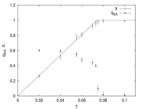
Figure 4: The quantities X and $q_{EA}$ for $t_{w}=2000$ as functions of the temperature. The straight line is the prediction of the approximation $X(T)=T/T_{eff}$.

The values of $X(C)$ and $q_{EA}$ obtained from this procedure are displayed in Fig. 4 as a function of $T$ using the data for $t_{w}=2000$ and $L=60$. We can see that at high temperatures $X$ is equal to $1$ and the usual FDT holds, whereas for $T<T_{eff}$ our results are well approximated by the straight line $X(T)=T/T_{eff}$ with $T_{eff}=0.074\pm 0.001$ . As the temperature increases the intersection point $q_{EA}$ decreases to zero with a sharp drop at $T_{eff}$ for this lattice size $L=60$. Our previous results Bekhechi and Southern (2003) for this model indicated a glass transition at a slightly lower temperature $T_{g}=0.071\pm 0.002$ where the relaxation time diverged. One would expect that $T_{eff}>T_{g}$ for systems with finite values of $L$ and $t_{w}$ and that it will approach $T_{g}$ for larger system sizes and longer waiting times. An extension of the present work to larger values of both $L$ and $t_{w}$ will also help to determine whether $q_{EA}$ approaches zero continuously or discontinuously at the glass transition.

In summary, we have shown that the fluctuation-dissipation ratio can be computed in this disorder free Kagome easy axis antiferromagnet. Several nontrivial features predicted by the mean field theory spin glasses are also present in this model. Namely, long-ranged memory effects and a constant FDR $X(C)$. These features correspond to a phase space structure similar to that of spin systems undergoing a one step replica symmetry breaking. The temperature dependence of the FDR $X(T)$ varies linearly with temperature $X(T)=T/T_{eff}$ as observed in binary mixtures of soft spheres Parisi (1997) and Lennard-Jones glasses Leonardo et al. (2000). All of our results are consistent with the existence of a glassy state at low temperatures in this geometrically frustrated model. The ideas developed for mean field descriptions of glassy systems seem to have an application far beyond the original models. Further experimental studies of these low dimensional frustrated magnets could provide some insight into the behaviour of glassy materials.