Inferring Pattern and Disorder in
Close-Packed Structures from X-ray Diffraction Studies, Part II:
Structure and Intrinsic Computation in Zinc Sulphide

Abstract

In the previous paper of this series [D. P. Varn, G. S. Canright, and J. P. Crutchfield, Physical Review B, submitted] we detailed a procedure—$\epsilon$-machine spectral reconstruction—to discover and analyze patterns and disorder in close-packed structures as revealed in x-ray diffraction spectra. We argued that this computational mechanics approach is more general than the current alternative theory, the fault model, and that it provides a unique characterization of the disorder present. We demonstrated the efficacy of computational mechanics on four prototype spectra, finding that it was able to recover a statistical description of the underlying modular-layer stacking using $\epsilon$-machine representations. Here we use this procedure to analyze structure and disorder in four previously published zinc sulphide diffraction spectra. We selected zinc sulphide not only for the theoretical interest this material has attracted in an effort to develop an understanding of polytypism, but also because it displays solid-state phase transitions and experimental data is available. With the first spectrum we find qualitative agreement with earlier fault-model analyses, although the reconstructed $\epsilon$-machine detects structures not previously observed. In the second spectrum, the results cannot be expressed in terms of weak faulting and so no direct comparison between the fault model and the reconstructed $\epsilon$-machine is possible. Nonetheless, we show that the $\epsilon$-machine gives substantially better experimental agreement and a number of structural insights. In the third spectrum, the fault model fails completely due to the high degree of disorder present, while the reconstructed $\epsilon$-machine reproduces the experimental spectrum well. In the fourth spectrum, we again find good quantitative agreement with experiment but find that the $\epsilon$-machine has difficulty reproducing the shape of several Bragg-like peaks. We discuss the reasons for this. Using the $\epsilon$-machines reconstructed for each spectrum, we calculate a number of physical parameters—such as, stacking energies, configurational entropies, and hexagonality—and several quantities—including statistical complexity and excess entropy—that describe the intrinsic computational properties of the stacking structures.

I Introduction

In the first paper Varn et al. (2003) of this two-part series we presented a novel technique for the discovery and description of planar disorder in close-packed structures (CPSs): $\epsilon$-machine spectral reconstruction theory ($\epsilon$MSR or “emissary”). We showed that the technique allows one to build the unique, minimal, and optimal model (an $\epsilon$-machine) of a material’s stacking structure from diffraction spectra. In this sequel we demonstrate the technique using diffraction spectra for disordered, polytypic zinc sulphide. Since the discovery of polytypism in mineral ZnS crystals by Frondel and Palache Frondel and Palache (1948, 1950) in 1948, much theoretical and experimental effort has been expended to understand this phenomenon. (See, for example, Steinberger, Steinberger (1983) Mardix, Mardix (1986) and Sebastian and Krishna. Sebastian and Krishna (1994)) ZnS is an attractive system to study for a number of reasons:

(i) Simplicity of the unit cell and stacking rules. While many materials are known to be polytypic, Trigunayat (1991); Sebastian and Krishna (1994) the constituent modular layers Varn and Canright (2001) (MLs) can have a complicated structure and complex stacking rules. Brindley (1980); J. B. Thompson (1983); Varn and Canright (2001) For instance, in ideal micas there are more than a dozen atoms in a unit cell, and there are six ways two MLs can be stacked. Kaolins and cronstedtites present even more complexity. Varn and Canright (2001) In contrast, ZnS is simple in the extreme: its basis is composed of but two atoms—a zinc and a sulphur. Sebastian and Krishna (1994) They are arranged in a double close-packed hexagonal net, with one species displaced relative to the other by a quarter body diagonal (as measured by the conventional unit cubic cell) along the stacking direction. Shaw and Heine (1990) We take this double close-packed layer to be a ML. Varn and Canright (2001) The stacking of MLs proceeds as for all CPSs; namely, there are three absolute orientations each ML can occupy—call them $A$, $B$, and $C$—with the familiar stacking constraint that no two adjacent MLs have the same orientation. Varn and Canright (2001)

(ii) Complex polytypism. ZnS is one of the most polytypic substances known with over 185 identified crystalline structures. Mardix (1986); Trigunayat (1991); Sebastian and Krishna (1994) Of these, only about a dozen fairly short-period polytypes (up to 21 MLs) are common in mineral ZnS, with the remainder found in synthetic crystals. Some of the crystal structures have repeat distances that extend over 100 MLs. Also, many structures show considerable planar disorder. The wide diversity of structural complexity remains one of the central mysteries of polytypism.

(iii) Solid-state transformations. It is believed that there are only two stable phases of ZnS, the low-temperature modification being the $\beta$-ZnS or sphalerite (3C not (a)) and the high-temperature modification wurtzite (2H) or $\alpha$-ZnS. Sebastian and Krishna (1994) The former transforms enantiotropically into the latter at 1024 C. The plethora of structures suggests that most of them are not in equilibrium but rather structures that are trapped in a local minimum of the free energy and lack the necessary activation energy to explore all of configuration space. It is possible to observe these structures by annealing and then arresting the transformation upon quenching. One can then study the various intermediate stages of the transformation.

(iv) Availability. Polytypes of ZnS, both ordered and disordered, are easily manufactured in the laboratory by a variety of methods. Sebastian and Krishna (1994) One of the more common is growth from the vapor phase above temperatures of about 1100 C. Crystals can also be grown from melt at high pressures, by use of chemical transport and hydrothermally. The distribution of polytypes observed depends on the method used.

Nearly a dozen theories have been proposed to explain polytypism, among them being the ANNNI model, Price and Yeomens (1984); Yeomans (1988) Jagodzinski’s disorder theory, Jagodzinski (1954) and Frank’s screw dislocation theory. Frank (1951) (For a complete discussion, see for example, Verma and Krishna, Verma and Krisha (1966) Trigunayat, Trigunayat (1991) and Sebastian and Krishna. Sebastian and Krishna (1994)) We will have little to say here about the mechanisms that produce various polytype structures. Instead, our focus will be on describing the disordered structures so commonly seen. We feel that an adequate description of the disordered structures—which so far has been lacking—is warranted before one can evaluate models that explain the formation of disorder and structures and, especially, the solid-state phase transitions that lead to them.

Previous descriptions of planar disorder in single crystals of ZnS fall into one of two categories: the fault model (FM) Varn et al. (2002, 2003) and Jagodzinski’s disorder model (DM). Jagodzinski (1949a, b, c); Frey et al. (1986) Applications of the FM include Roth’s Roth (1960) study of faulting induced in hexagonal crystals grown from the vapor phase upon annealing. Roth extracted correlation information from the diffraction spectra by Fourier analysis and then derived analytical expressions relating how correlation functions decayed with both increasing separation between MLs and as a function of the fault probability. He considered both randomly distributed growth and deformation faults and found that for weakly disordered specimens deformation faulting gave the best agreement with experiment.

Significant applications of the FM to planar disorder in ZnS have been carried out by Sebastian, Krishna, and coworkers. They studied the 2H-to-3C solid-state transformation in vapor-grown ZnS crystals after annealing between temperatures of 300 to 650 C. Sebastian et al. (1982) By analyzing and comparing the profiles of the integer-$l$ reflections not (b) to those of the half-integer-$l$ reflections for weakly faulted crystals, they found that the disorder was largely due to the random insertion of deformation faults. They attributed slight discrepancies between the observed and calculated profiles to the so-called nonrandom insertion of faults. Sebastian and Krishna Sebastian and Krishna (1984) later studied the disordered stacking in 3C crystals grown from the vapor phase, as well as those obtained from annealing 2H crystals. They found that the structure of both the as-grown and annealed crystals was best explained as randomly distributed twin faults in the 3C structure. They concluded that the 2H-to-3C transformation in ZnS proceeded by the nonrandom nucleation of deformation faults occurring preferentially at two ML separations.

To better understand the nature of the nonrandom insertion of deformation faults in the 2H structure, Sebastian and Krishna Sebastian and Krishna (1987a, b) introduced a three-parameter model that assigned separate probabilities to the random insertion of deformation faults, as well as deformation faulting at two and three ML separations. They derived analytical expressions for the diffraction spectra in terms of these parameters and concluded that both the 2H-to-3C and the 2H-to-6H transformations proceeded via the nonrandom nucleation of deformation faults. Their analysis showed that these transformations occurred simultaneously in different regions of the same crystal. They attributed this to variations in the stoichiometry. Sebastian Sebastian (1988) gave a similar treatment that came to the same conclusions. With the exception of Roth, all of these analyses depended on carefully characterizing the change in Bragg peaks as one introduces a small amount of disorder. We have previously given a criticism of the FM approach elsewhere. Varn et al. (2002, 2003)

Jagodzinski’s DM is a two-parameter model that assumes two thermodynamically stable phases in CPSs: the 2H and 3C. One therefore finds two kinds of fault (and here we mean structure and not mechanism): namely, cubic faults in the 2H and hexagonal faults in the 3C. By choosing appropriate values of the two model parameters one can also model 4H structures. Within this framework, an analytical expression for the diffracted intensity is derived that depends on the model parameters in a complicated manner. Nonetheless, one can select model parameters that give the best agreement with experiment.

Müller Müller (1952) used this method to analyze faulted ZnS diffraction spectra and found that while he was able to obtain reasonable agreement between theory and experiment for a few spectra, for many he was not. Singer Singer and Gashurov (1963) re-examined this approach and concluded that the DM applies when faulting is random, but when the faulting is nonrandom, as many ZnS specimens are suspected to be, the model fails. However, Frey et al. Frey et al. (1986) studied the 3C-to-2H transformation in single crystals of ZnS using the DM and were able to obtain excellent agreement between theory and experiment. They fitted the experimental diffraction spectra to the DM’s analytical one. Due to the complicated nature of the expression, however, they treated eight constants that depend on the two model parameters as independent. From these eight fitted parameters they were able to find the two model parameters that best fit each spectra.

One cannot help but raise questions concerning the mathematical rigor used to find the model parameters in this way. We show elsewhere Varn et al. that the description of the stacking disorder as given by the DM is a special constrained case of the ${r}=2$ computational mechanics approach. As in the latter, in the DM there is no assumption of weak faulting and one does use diffuse scattering to build the model. Since the spectra we analyze have not been previously treated using the DM and it is a special case of our own, we do not discuss the DM further here, but treat it in detail elsewhere. Varn et al.

A third possible method of discovering structural information about disordered solids from diffraction spectra employs a reverse Monte Carlo (RMC) technique. Proffen and Welberry (1998); Welberry and Proffen (1998) In this method, one typically searches for a configuration of constituent atoms such that a signal—e.g., the diffraction spectrum—estimated from the candidate structure most closely matches the experimental signal. This technique can be applied for the case of disorder in three dimensions. One drawback, however, is that candidate structures are often found that are physically implausible. One needs to impose assumptions to eliminate these. To our knowledge, this technique has not been applied to polytypism, and we do not consider it here.

In this work, we apply computational mechanics Crutchfield and Young (1989); Feldman and Crutchfield (1998); Shalizi and Crutchfield (2001) to discover and describe disordered stacking sequences in four previously published ZnS diffraction spectra. We Fourier analyze each spectrum to find correlation information between MLs and then calculate the probability distribution of stacking sequences. From the latter, we reconstruct the $\epsilon$-machine that gives the stochastic process for the ML stacking and compare it to previous FM analyses. From the reconstructed $\epsilon$-machine, we calculate the stacking entropy per layer, average stacking-fault energy per Zn-S pair, memory length, hexagonality, and generalized period. Varn et al. (2003) We find that the diffraction spectra of the four samples is well described using the computational mechanics approach.

We note that our primary purpose in the following is expository; that is, we wish to demonstrate the efficacy of $\epsilon$MSR on real data. Since we use diffraction spectra from older studies, Sebastian and Krishna (1994) the analyses given here are less than ideal. Specifically, we digitized data from the published spectra and found that there was significant systematic error in each spectrum. Additionally, the experimental data was not reported with error bars. Despite these possible shortcomings, $\epsilon$MSR allows us to offer more comprehensive analyses of the spectra than given by previous workers.

Our development is organized as follows. In §II we outline our approach, including a brief discussion of the experimental methods and our analysis. In §III, we give the results of $\epsilon$-machine reconstruction for four experimental ZnS diffraction spectra and contrast this to the FM approach when possible. In §IV we calculate the stacking energies per Zn-S pair and the hexagonality for the various structures from our reconstructed $\epsilon$-machines. In §V we give our conclusions and propose some directions for future theoretical and experimental work.

II Methods

The four diffraction spectra we analyze come from Sebastian and Krishna Sebastian and Krishna (1994) and are labeled SKXXX by the page (XXX) on which they appear in that source. These data were collected in the 1980’s and since they no longer exist in numerical form, Sebastian we digitized them from the diffractograms given in the Sebastian and Krishna publication. Sebastian and Krishna (1994) In this section, we give a brief synopsis of the experimental procedure, discuss the assumptions made to analyze the data, and list the corrections we apply to the experimental spectra.

II.1 Experimental Details

The experimental procedure is given in more detail elsewhere.Sebastian and Krishna (1994); Sebastian et al. (1982); Sebastian and Krishna (1987b); Sebastian (1988) Briefly, the crystals were grown from the vapor phase at a temperature in excess of 1100 C in the presence of H₂S gas. Each crystal was needle-shaped, approximately 0.1 to 0.4 mm in diameter and 1 to 2 mm in length. Two of the four crystals were further annealed for one hour at 300 and 500 C. These investigations were performed to better understand the fault structures they contain, as well as study the solid-state transformations that ZnS crystals undergo.

The intensity along the $10.l$ reciprocal lattice row was recorded using a four-circle single-crystal diffractometer for each specimen in steps of approximately $\Delta l=0.005$. (Our definition of $l$ differs slightly from that of Sebastian and Krishna, Sebastian and Krishna (1994) so the $l$-increment we report also differs.) The crystal and the counter were held stationary while the crystal was illuminated with Mo$K_{\alpha}$ radiation. The sharp reflections along the $h-k=0\mod 3$ rows were used to orient each crystal. The divergence of the incident beam was adjusted to cover the mosaic spread for each crystal. The experimental diffraction spectrum is reported as the total number of counts versus $l$. The crystals were examined under a vickers projection microscope and did not show signs of kinking or shearing, even after annealing. They did show parallel striations or stripes perpendicular to the stacking direction.

II.2 Assumptions

To make the analysis tractable, we employ the following assumptions common in the analysis of planar disorder in ZnS:

(i) Each ML is perfect and free of distortions and defects. We assume that each ML is identical and the MLs themselves are undefected. That is, each ML is crystalline in the strict sense, with no point defects, impurities, or distortions in the two-dimensional lattice structure. This clearly precludes the possibility of screw dislocations, which are known to play a role in the polytypism of some ZnS crystals. Sebastian and Krishna (1994); Michalski (1988) Since each of the crystals we analyze was examined under a vickers projection microscope and no such dislocations were seen, and the crystals retained their shape after annealing, this seems reasonable. (It is known Sebastian and Krishna (1994) that during solid-state transformations of specimens of ZnS with an axial screw dislocation the specimen will exhibit ”kinking” with a characteristic angle of $19^{0}28^{\prime}$.)

(ii) The spacing between MLs is independent of the local stacking arrangement. There is known to be some slight dependence of the inter-ML spacing depending on the polytype. Sebastian (1988); Sebastian and Krishna (1994) For the 2H structure in ZnS, the inter-ML spacing is measured to be 3.117 Å. For the 3C structure, the cubic cell dimension is $a_{c}=5.412$ Å which gives a corresponding inter-ML spacing of 3.125 Å. Therefore, to an excellent approximation, this spacing is independent of the local stacking environment in ZnS.

(iii) The scattering power of each ML is the same. We assume that each ML diffracts x-rays with the same intensity. There is no reason to believe that this is not so, unless absorption effects are important or the geometry of the crystal is such that each ML does not have the same cross-sectional area.

(iv) The stacking faults extend over the entire fault plane. Examination under microscope indicates that this is generally true. However, Akizuki Akizuki (1981) found evidence that the faults do not extend completely over the faulted MLs by examining a partially transformed ZnS crystal under an electron microscope.

(v) We assume that the “stacking process” is stationary. We simply mean that the faults are uniformly distributed though out the crystal. Put another way, we assume that probability of finding a particular stacking sequence is independent of its location in the crystal. This does not, however, preclude regions of crystal structure interspersed between regions of disorder. It simply means that the statistics of the stacking does not change as one moves from one end of the crystal to the other.

Notably absent from this list are any assumptions about the crystal structure present (if any) and how the sample might deviate from that structure. In contrast to the FM, we invoke no a priori structural assumptions concerning the stacking sequence.

II.3 Corrections to the Experimental Spectra

We corrected each spectrum for the following effects:

(i) The atomic scattering factor. This correction accounts for the spatial distribution of electrons, as well as for the wavelength of the incident radiation and angle of reflection. Calculations of these effects are given in standard tables Hahn et al. (1992) and we employ them in our work.

(ii) The structure factor. The structure factor Sebastian and Krishna (1994) accounts for the two-atom basis in ZnS.

(iii) Anomalous scattering factors. Also called dispersion factors, the anomalous scattering factors correct for the binding energy of the electrons and the phase shifts. Hahn et al. (1992) For our case, we find these to be small, but have included them nonetheless.

(iv) Polarization factor. We use the standard correction factor for unpolarized radiation. Warren (1969)

Factors we did not correct for include the following:

(i) Thermal factors. At room temperature, this effect is small for ZnS. Varn (2001)

(ii) Absorption factor. For the geometry of the ZnS crystals we analyze, the linear mass coefficient Woolfson (1997); Milburn (1973) is much larger than the thickness, therefore we ignore it.

(iii) Instrument resolution. This is not reported with the experimental data, so we do not deconvolve the spectrum.

III Analysis

We now give the structural analysis of four experimental diffraction spectra taken from Sebastian and Krishna. Sebastian and Krishna (1994) We apply $\epsilon$MSR to each to build a model that describes the stacking process. From our model, we calculate various measures of intrinsic computation for each spectra. We compare our results with that obtained by previous researchers using the FM. Since the experimental spectra are not reported with error bars, we are unable to set an error threshold $\Gamma$ as required in $\epsilon$MSR. Instead, we found that each increase in the memory length ${r}$ continues to give a better description of each spectra. Varn (2001) We perform $\epsilon$-machine reconstruction up to ${r}=3$ for each spectra. To find the CFs from the $\epsilon$-machines, we take a sample length 400 000, as generated by the $\epsilon$-machine. The diffraction spectra are calculated using 10 000 MLs. The experimental spectra are normalized to unity over the $l$-interval used for reconstruction, as are the spectra calculated from each $\epsilon$-machine. For the spectra calculated from the FM, we set the overall scale to best describe the Bragg peaks as shown in Sebastian and Krishna. Sebastian and Krishna (1994) We also calculate the profile ${\cal R}$-factor Varn et al. (2003) to evaluate the agreement between experiment and theory for each spectrum.

III.1 SK134

Figure 1: Diffraction spectrum along the $10.l$ row from SK134 corrected for atomic scattering factors, the structure factor, dispersion factors, and the polarization factor. Hahn et al. (1992); Woolfson (1997); Warren (1969) We see that the spectrum is not periodic in $l$, as it should be. This indicates that there exist significant errors in the data.

The corrected diffraction spectrum along the $10.l$ row for an as-grown 2H ZnS crystal is shown in Fig. 1. One immediately notices that the spectrum is not periodic in $l$, as it should be, but instead suffers from variations in the intensity. The peaks at $l=0.0$ and $l=1.0$ are of similar intensity, but the peaks at $l=-0.5$, 0.5 and 1.5 seem to suffer from a steady decline in intensity. We can therefore be confident that this spectrum contains substantial systematic error as reported by the experimentalists.

This difference in diffracted intensity between peaks results from the finite thickness of the Ewald sphere due to the divergence of the incident beam. Sebastian and Krishna (1987b, 1994) A suitable choice of geometry can minimize, but not eliminate these effects, such that one finds only a gradual variation in $I$ with $\Delta l$. Since analysis by the FM depends only on the change of the shape and the position of the Bragg-like peaks, such a slow variation of the diffracted intensity with $l$ will not affect the conclusions drawn from an FM analysis. It is possible to correct these effects, Pandey et al. (1987); Sebastian and Krishna (1994) but this has not been done in the literature.

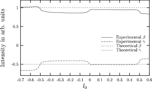
Figure 2: Experimental and theoretical figures-of-merit—$\beta$ and $\gamma$—as a function of $l_{0}$ for diffraction spectrum SK134. We define $l_{0}$ as the point at which integration over a unit $l$-interval is initiated. We see that $l_{0}\approx 0.04$ gives the best agreement with the theoretical values.

Our analysis depends on selecting an appropriate $l$-interval where variations in diffracted intensity due to these experimental effects are minimized. It is important, then, to select an interval that is relatively error-free. As discussed in Part I,Varn et al. (2003) there are two criteria, called figures-of-merit and denoted $\gamma$ and $\beta$, one can use for this. It can be shown that in an error-free spectrum the parameters must be equal to constant values $-1/2$ and $1$, respectively, for any unit $l$-interval, regardless of the amount of planar disorder present. The extent that $\beta$ and $\gamma$ differ from their theoretical values over a given $l$-interval measures how well the diffraction spectrum over the interval can be represented by a physical stacking of MLs. It makes sense, then, to choose an $l$-interval for $\epsilon$-machine reconstruction such that the theoretical values of the figures-of-merit are most closely realized. This does not, of course, guarantee that the interval is error-free. Glancing at Fig. 2 shows that $\gamma=-0.51$ and $\beta=0.95$ over the interval $l\in[0.04,1.04]$.

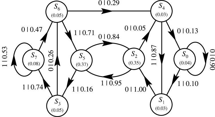
Figure 3: The ${r}=3$ $\epsilon$-machine reconstructed for SK134. The recurrent causal states $\{{\cal S}_{0}\ldots{\cal S}_{7}\}$ are labeled (in decimal notation) by the last three (binary) spins seen and the asymptotic state probabilities are given for each state. Edge labels $s|p$ indicate a transition on spin $s$ with probability $p$. The large asymptotic state probabilities for the ${\cal S}_{2}$ and ${\cal S}_{5}$ states, as well as the large state-transition probabilities between them, show that this is predominately a 2H crystal with some faulting.

We perform $\epsilon$MSR Varn et al. (2003) and find that the smallest-$r$ $\epsilon$-machine that gives reasonable agreement between the measured and $\epsilon$-machine spectra has a memory length of ${r}=3$. The reconstructed $\epsilon$-machine is shown in Fig. 3. The large asymptotic state probabilities for the ${\cal S}_{2}$ and ${\cal S}_{5}$ causal states (CSs), as well as the large inter-state transition probabilities between them, indicate this is predominantly a 2H crystal. More specifically, the probability of seeing sequences 1010 and 0101, corresponding to the 2H cycle, have a combined total weight of about $64\%$. The remaining probability is distributed among the other fourteen length-$4$ sequences. It is tempting to interpret the remaining structure in terms of faults and, indeed, it seems we can.

Let us treat the transitions $s=0$ from ${\cal S}_{4}$ and $s=1$ from ${\cal S}_{0}$ as though they are missing for the purposes of a fault analysis. This implies that the sequences $0001$ and $1000$ are disallowed. Of course, this cannot be exactly true, as the CS ${\cal S}_{0}$ would then be isolated from the rest of the $\epsilon$-machine. In this case, we would say that the $\epsilon$-machine is not strongly connected and, as such, cannot represent a physical stacking of MLs. However, the combined probability weight of these two sequences is $<1\%$, so neglecting them gives only a small error in our intuitive understanding of the faulting structure.

Then on the left half of the $\epsilon$-machine there is structure associated with a 2H deformation fault $[{\cal S}_{3}{\cal S}_{7}{\cal S}_{6}{\cal S}_{5}]$ with probability weight $0.16={\rm P}(1011)+{\rm P}(0111)+{\rm P}(1110)+{\rm P}(1101)$. We can interpret the causal-state cycle (CSC) $[{\cal S}_{3}{\cal S}_{6}{\cal S}_{4}{\cal S}_{1}{\cal S}_{2}{\cal S}_{5}]$ as a layer-displacement fault and see that it is assigned a probability weight of $0.06$. The right portion contains the CSC $[{\cal S}_{4}{\cal S}_{1}{\cal S}_{2}]$ with probability weight $0.06$, which is associated with growth faults. The CSCs $[{\cal S}_{0}]$ and $[{\cal S}_{7}]$, identified as 3C structure, have a combined weight of $0.08$.

Given these observations, a possible interpretation suggested by the $\epsilon$-machine is that SK134 has crystal structures and faults in the proportions given in Table 1. The decomposition there is sensible since there is an underlying crystal structure present and the smaller, faulting paths are not too large. As we will see, these need not always be the case. Sebastian and Krishna Sebastian and Krishna (1994) have analyzed this diffraction spectrum using the FM and found that approximately one in every twenty MLs is deformation faulted, so they described the stacking structure as a faulted 2H crystal with 5% random deformation faulting. This is equivalent to assigning CSCs responsible for deformation faulting a total probability weight of 0.17. We compare the structure analyses of the two models in Table 1.

Structure	$\epsilon$-Machine	Fault Model
2H	$64\%$	$83\%$
3C	$8\%$	$0\%$
Deformation fault	$16\%$	$17\%$
Growth fault	$6\%$	$0\%$
Layer-displacement fault	$6\%$	$0\%$

Table 1: Structural decomposition of SK134 according to the reconstructed $\epsilon$-machine of Fig. 3 and according to the fault model analysis of Sebastian and Krishna. Sebastian and Krishna (1994) The latter is valid only under the assumption of weak faulting.

We see that both analyses agree that the dominant structure is 2H, though the $\epsilon$-machine attributes less of the crystal structure to this “parent” phase. Similarly, both find that structures associated with deformation faulting are important and assign them almost equal weights.

They differ, however, in that the $\epsilon$-machine finds additional faulting structures (growth and layer-displacement faulting), as well as 3C crystal structure. Since this crystal, if annealed at sufficient temperatures for a long enough time, will transform into a twinned 3C structure, the latter is easily understood as nascent structure in that process. Finding the presence of weak 3C structure is not unreasonable since there is some slight enhancement of the diffracted intensity at $l\approx 1/3$ and $l\approx 2/3$. The other faulting structures seen are less easily understood. Growth faults, so-named because they primarily are formed during the growth of the 2H crystal, are not expected to play an important role in solid-state transformations of ZnS. Roth (1960) Their presence here may result from the initial growth of the crystal. The small amount of layer-displacement structure could be seen as two adjacent, yet oppositely oriented deformation faults. That is, a deformation fault in a 2H structure is simply a spin flip in the Hägg notation, Varn et al. (2003) so that a sequence $\ldots 010101\ldots$ transforms to $\ldots 01\underline{1}101\ldots$ as a result of one deformation and then to $\ldots 011\underline{0}01\ldots$ upon another resulting in a layer-displacement fault $\ldots 01\underline{10}01\ldots$. This might imply some coordination between faults. Or, the mechanism of layer-displacement faulting may play some minor role in the solid-state transformation.

However, one cannot disambiguate these from the available spectra and the reconstructed $\epsilon$-machine. The $\epsilon$-machine only provides information about the structure. We must look outside the $\epsilon$-machine to formulate an understanding of how the polytype came to be stacked in this way. This is the critical difference between faulting mechanism and faulting structure. In the former, a physical process is responsible for causing the MLs to shift or deviate from a perfect crystal. In the latter, in the limit of weak faulting, the physical process leads to a given (statistical) structure. In this limit it may be possible to postulate with some certainty that the mechanism resulted in the observed structure. For more heavily faulted crystals, however, such an identification of structure with mechanism is dubious. Other techniques, such as numerical simulations Kabra and Pandey (1988); Engel (1990); Shrestha et al. (1996); Shrestha and Pandey (1996a, b, 1997); Gosk (2000, 2001) or analysis of a series of crystals in various stages of the transformation, are necessary to unambiguously determine the mechanism.

Figure 4: $Q_{s}(n)$ versus $n$ for experimental spectrum SK134 (open squares connected by solid line), the fault model (open circles), and the ${r}=3$ $\epsilon$-machine (solid squares). The $Q_{s}(n)$ are defined only for integer values of $n$, but lines are drawn connecting adjacent points as an aid to the eye. We see good agreement up to $n\approx 15$, after which the ${r}=3$ approximate correlation functions die too quickly to their asymptotic value of $1/3$.

Returning to the analysis of SK134, Fig. 4 compares the CFs obtained from the experimental diffraction spectrum, those obtained from the $\epsilon$-machine and those from the FM. There is reasonable agreement between the experimental and $\epsilon$-machine-predicted CFs. For small $n$, however, the FM overestimates the amplitude in the oscillations in $Q_{s}(n)$. The experimental diffraction spectrum is compared to that calculated from the FM and $\epsilon$-machine in Fig. 5. Both models give good agreement near the Bragg peaks at $l=0.5$ and $l=1.0$, with perhaps the FM performing a little better at $l=1.0$. The diffuse scattering near the shoulders of the $l=0.5$ peak are better represented by the $\epsilon$-machine. We calculate the profile ${\cal R}$-factor between experiment and the FM to be ${\cal R}_{\mathrm{FM}}=33\%$ and between experiment and $\epsilon$MSR to be ${\cal R}_{\epsilon M}=20\%$.

From the $\epsilon$-machine we calculate the three length parameters to be ${r}=3$ ML, $\mathcal{P}=4.8$ ML, and $\lambda_{c}=9.5\pm 0.5$ ML. The three measures of intrinsic computation are found to be ${h_{\mu}}=0.50$ bits/ML, ${C_{\mu}}=2.3$ bits, and ${\bf E}=0.75$ bits. We return to discuss and compare these for all of the samples in a later section.

Figure 5: Comparison of the experimental diffraction spectrum SK134 along the $10.l$ row (triangles) for a disordered ZnS single crystal with a spectra estimated from the FM with $5\%$ deformation faulting (dashed line) and ${r}=3$ $\epsilon$-machine (solid line). The vertical scale in the inset is logarithmic intensity. For clarity, we report only a few representative data points from the experimental diffraction spectrum. In our analysis, however, we used the much finer mesh reported in the experimental data. We find that the $\epsilon$MSR gives ${\cal R}_{\epsilon M}=20\%$, while the FM gives ${\cal R}_{\mathrm{FM}}=33\%$.

III.2 SK135

Figure 6: Comparison of the experimental diffraction spectrum SK135 along the $10.l$ row (triangles) for a disordered 3C single crystal with the diffraction spectra calculated from the FM with $12\%$ twinned faulting (dashed line) and the $\epsilon$-machine (solid line). We find that the $\epsilon$MSR gives ${\cal R}_{\epsilon M}=13\%$, while the FM gives ${\cal R}_{\mathrm{FM}}=33\%$.

The next sample we examine is a twinned 3C crystal obtained by annealing a 2H crystal at 500 C for 1 h. The diffraction spectrum for this crystal is given in Fig. 6. We find that figures-of-merit are closest to their theoretical values over the interval $l\in[-0.80,0.20]$ with values $\beta=-0.50$ and $\gamma=0.93$. The smallest-$r$ $\epsilon$-machine that gives reasonable agreement with experiment was found at ${r}=3$ and has a profile ${\cal R}$-factor of ${\cal R}_{\epsilon M}=13\%$. The resulting $\epsilon$-machine is shown in Fig. 7. Based on the presence of asymmetrically broadened peaks and the absence of peak shifts, a FM analysis Sebastian and Krishna (1994) finds this sample to be a twinned 3C crystal with $12\%$ twinned faulting. The profile ${\cal R}$-factor between experiment and the FM is found to be ${\cal R}_{FM}=33\%$.

The large CS probabilities associated with CSs ${\cal S}_{0}$ and ${\cal S}_{7}$, as well as their large self-loop transition probabilities, suggest that this is a twinned 3C crystal. We also note that the transitions corresponding to antiferromagnetic paths ($0101$ and $1010$) have a relatively small combined weight of only about $4\%$. In fact, the probability weight for the $0101$ path is zero. (The transition from ${\cal S}_{2}$ to ${\cal S}_{5}$ is missing.) This indicates that 2H structure has largely been eliminated. In addition to the $0101$ path, the $1001$ and $0010$ paths are also missing. This implies that twinned faulting is important, but also the remnant of the $1010$ path has some role. Instead of a simple twinned fault $[{\cal S}_{7}{\cal S}_{6}{\cal S}_{4}{\cal S}_{0}]$ giving the sequence $\ldots 1111|0000\ldots$, where the vertical line indicates the fault plane, the path $[{\cal S}_{7}{\cal S}_{6}{\cal S}_{5}{\cal S}_{2}{\cal S}_{5}{\cal S}_{0}]$ giving the sequence $\ldots 1111|01000\ldots$ has approximately twice as much probability weight associated with it. In the $\epsilon$-machine’s right portion twinned faulting $[{\cal S}_{0}{\cal S}_{1}{\cal S}_{3}{\cal S}_{7}]$ is largely responsible for the $(0)^{*}$ 3C cycle converting to the $(1)^{*}$ 3C cycle and we also observe that double deformation faulting $[{\cal S}_{0}{\cal S}_{1}{\cal S}_{3}{\cal S}_{6}{\cal S}_{4}]$ plays a role.

It is interesting to mention that, while a ML of ZnS has spin-inversion symmetry Varn and Canright (2001) and, thus, the one-dimensional Hamiltonian describing the energetics of the stacking is also spin invariant, in general $\epsilon$-machines need not be spin-inversion invariant. [Note that the $\epsilon$-machine in Fig. 7 is not spin-inversion invariant.] There is, of course, no reason why we should demand spin-inversion invariance. After all, then one could never have a crystal of purely one 3C structure or the other. However, since this crystal was initially in the 2H structure—which is spin-inversion invariant—it is curious that this is not preserved as the crystal is annealed. That is, there is no reason to expect that faulting should occur preferentially with one chirality. Notably, the FM always assumes spin-inversion symmetry.

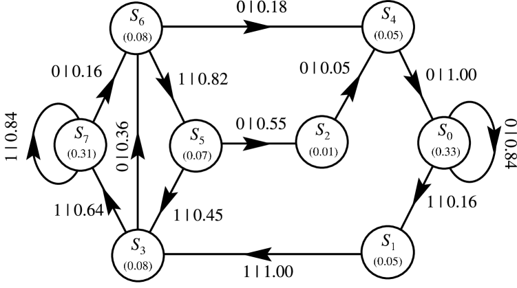
Figure 7: The reconstructed ${r}=3$ $\epsilon$-machine for SK135. The strong self-loop transition probabilities between causal states ${\cal S}_{0}$ and ${\cal S}_{7}$ as well as their large asymptotic state probabilities indicate that the $\ldots 0000\ldots$ and $\ldots 1111\ldots$ structures are important. This, then, is a twinned 3C crystal.

Examining the $Q_{s}(n)$ estimated from experiment with those found from the $\epsilon$-machine in Fig. 8, we find reasonable agreement up to $n\approx 20$. The $Q_{s}(n)$ found from the FM generally overstate the magnitude of the oscillations in the CFs.

We can further examine the diffraction spectra. In Fig. 6, the diffraction spectrum found from the FM and the $\epsilon$-machine are compared with experiment. The $\epsilon$-machine gives a good fit, except perhaps at a shoulder in the experimental spectrum at $l=-0.6$ and the small rise at $l=-0.16$. The latter might be understood as a minor competition between the 3C and 6H CSCs that is not being well modeled at ${r}=3$. Comparison of the diffraction spectrum from the FM with that from experiment reveals good agreement with the peak at $l=-0.33$ and poor agreement with the one at $l=-0.67$. This is not surprising as the FM did not use the peak at $l=-0.67$ to find the faulting structure. Likewise, the diffuse scattering between peaks is not at all well represented by the FM. Additionally, the small rise in diffuse scattering at $l=-0.16$ is likewise absent in the FM diffraction spectrum.

From the $\epsilon$-machine we calculate the three length parameters to be ${r}=3$ ML, $\mathcal{P}=5.6$ ML, and $\lambda_{c}=4.4\pm 0.7$ ML. The three measures of intrinsic computation are found to be ${h_{\mu}}=0.59$ bits/ML, ${C_{\mu}}=2.5$ bits, and ${\bf E}=0.71$ bits.

Figure 8: Comparison of the $Q_{s}(n)$ versus $n$ for experimental spectrum SK135 (open squares), the $\epsilon$-machine (solid squares), and the FM (open circles). The $\epsilon$-machine gives good agreement with experiment, while the FM overestimates the oscillation magnitude.

III.3 SK137

Figure 9: Comparison of the experimental diffraction spectrum SK137 along the $10.l$ row (triangles) for a disordered 3C single crystal with the diffraction spectra calculated from the FM with $6.8\%$ twinned faulting (dashed line) and the $\epsilon$-machine (solid line). The profile ${\cal R}$-factor between experiment and the $\epsilon$-machine calculated diffraction pattern is ${\cal R}_{\epsilon M}=17\%$. The FM gives considerably worse agreement, with a calculated profile ${\cal R}$-factor of ${\cal R}_{FM}=58\%$ between it and experiment.

The third experimental spectrum we analyze comes from an as-grown disordered, twinned 3C crystal. The diffraction spectrum for this crystal along the $10.l$ row is shown in Fig. 9. The figures-of-merit are closest to their theoretical values over the interval $l\in[-0.8,0.2]$ with values of $\gamma=-0.49$ and $\beta=0.98$. We performed $\epsilon$-machine reconstruction up to ${r}=3$ and found that this produces reasonable agreement with experiment giving a profile ${\cal R}$-factor of ${\cal R}_{\epsilon M}=17\%$. The ${r}=3$ approximate $\epsilon$-machine in shown in Fig. 10. A FM analysis finds SK137 to be a twinned 3C crystal with $6.8\%$ twinned faulting. Sebastian and Krishna (1994) The FM-calculated diffraction spectrum has a profile ${\cal R}$-factor of ${\cal R}_{\epsilon M}=58\%$ when compared with experiment.

A comparison of the CFs from experiment, the FM, and the $\epsilon$-machine is shown in Fig. 11. For smaller $n$, the $\epsilon$-machine gives good agreement with experiment, although the error increases at larger $n$. As shown elsewhere, Varn (2001) the experimental CFs maintain small, but persistent oscillations about their asymptotic value of $1/3$ up to $n\approx 40$, while the CFs derived from the $\epsilon$-machine effectively reach this asymptotic value at $n\approx 25$. This leads us to speculate that there is some structure in the stacking process that the $\epsilon$-machine is missing. We expect that reconstruction at ${r}=4$ will prove interesting here. This has not yet been completed.

The FM fares markedly worse. It substantially overestimates the strength of the oscillations in the CFs for all $n$.

A comparison of the diffraction spectra for experiment, the FM, and the $\epsilon$-machine is given in Fig. 9. The $\epsilon$-machine gives reasonable agreement everywhere except around the Bragg peaks at $l=-0.33$ and $l=-0.67$. Here the $\epsilon$-machine gives a value for the peak intensity $15\%$ and $35\%$ lower, respectively, than experiment. The FM does much better at the Bragg peaks, as one might expect. The diffuse scattering between the peaks, and especially the broad-band rise in intensity near $l=-0.5$, are simply missing in the FM diffraction spectrum, however. The $\epsilon$-machine fit in this region is substantially better, picking up a number of important spectral features, such as broadband components and broadened peaks.

Figure 10: The reconstructed ${r}=3$ $\epsilon$-machine for SK137. The strong self-loop transition probabilities between causal states ${\cal S}_{0}$ and ${\cal S}_{7}$, as well as their large asymptotic state probabilities, suggest that the $\ldots 0000\ldots$ and $\ldots 1111\ldots$ structures are important. Notice that, unlike the $\epsilon$-machine for SK135, the CSC $[{\cal S}_{2}{\cal S}_{5}]$ is present, suggesting that associated 2H structure is present. The absence of the transition between CSs ${\cal S}_{1}$ and ${\cal S}_{3}$ implies that the $0011$ sequence, and therefore the CSC associated with the 6H structure, is not present.

What does the $\epsilon$-machine imply about the stacking process? All CSs and allowed transitions are present except for the transition between ${\cal S}_{1}$ and ${\cal S}_{3}$. This absent transition implies that the $0011$ stacking sequence is not present in SK137. This, then, means that the $000111$ sequence, and hence the CSC $[{\cal S}_{7}{\cal S}_{6}{\cal S}_{4}{\cal S}_{0}{\cal S}_{1}{\cal S}_{3}]$ associated with the 6H structure,Varn et al. (2003) is also absent. Therefore, in this twinned 3C crystal there is no 6H structure. This is surprising, since many ZnS spectra show enhancement about the 6H positions during solid-state phase transitions from 2H to 3C. In Fig. 9 there is (arguably) a slight increase in diffracted intensity at $l=-0.16$ and $l=0.16$. So the absence of the 6H structure does seem echoed in the experimental spectrum. There is, however, a large broadband increase in intensity about $\l=-0.5$ and a much smaller increase about $\l=0.0$. Reflections at these $l$ are usually associated with 2H structure, with the half-integer peaks carrying three times the intensity of the integer peaks. The $\epsilon$-machine does show that the CSC $[{\cal S}_{2}{\cal S}_{5}]$ associated with the 2H structure is present. The frequency of occurrence of the 0101 and 1010 stacking sequences together make up about $12\%$ of the total probability weight on the $\epsilon$-machine. Even though $P_{CSC}([{\cal S}_{2}{\cal S}_{5}])\ll 1$, it is not unreasonable to suggest that 2H structure is present.

Figure 11: Comparison of the $Q_{s}(n)$ versus $n$ for experimental spectrum SK137 (open squares), the ${r}=3$ approximate $\epsilon$-machine (solid squares), and the FM (open circles).

As with the other spectra, we can calculate several characteristic length and information- and computational-theoretic quantities from the $\epsilon$-machine. We find the three length parameters to be ${r}=3$ ML, $\mathcal{P}=6.7$ ML, and $\lambda_{c}=12\pm 3$ ML. The three measures of intrinsic computation are found to be ${h_{\mu}}=0.65$ bits, ${C_{\mu}}=2.7$ bits, and ${\bf E}=0.79$ bits.

III.4 SK229

Figure 12: A comparison of the experimental diffraction spectrum SK229 (dashed line) and that calculated from the reconstructed $\epsilon$-machine (solid line). There is generally good agreement between two, except that the Bragg-like peaks from the $\epsilon$-machine are slightly displaced from the experimental spectra and the maximum from the $\epsilon$-machine overestimates experiment. The $\epsilon$-machine also has some difficulty reproducing the shape of the experimental spectra. The profile ${\cal R}$-factor between the two spectra is ${\cal R}_{\epsilon M}=29\%$.

Lastly, we examine an as-grown 2H crystal. The diffraction spectrum for this crystal is shown in Fig. 12. We find the figures-of-merit closest to their theoretical values over the interval $l\in[-0.33,0.67]$ with values of $\gamma=-0.49$ and $\beta=1.00$. We find that the smallest-$r$ $\epsilon$-machine that gives reasonable agreement between the measured and $\epsilon$-machine spectra has a memory length of ${r}=3$. The reconstructed $\epsilon$-machine is shown in Fig. 13. The large asymptotic state probabilities for the ${\cal S}_{2}$ and ${\cal S}_{5}$ CSs, as well as the large inter-state transition probabilities between them, indicate this is predominantly a 2H crystal. More specifically, the probability of seeing sequences 1010 and 0101, corresponding to the 2H cycle, have a combined total weight of about $82.5\%$. The remaining probability is distributed among the other fourteen length-$4$ sequences. It is tempting to interpret the remaining structure as faults and, indeed, we can.

Let us treat the transitions $s=0$ from ${\cal S}_{6}$ and $s=1$ from ${\cal S}_{1}$ as though they are missing. These are the least probable transitions in the $\epsilon$-machine: ${\rm P}(0,{\cal S}_{6})={\rm P}({\cal S}_{6}){\rm P}(0|,{\cal S}_{6})\approx 0.004$ and ${\rm P}(1,{\cal S}_{1})={\rm P}({\cal S}_{1}){\rm P}(1|,{\cal S}_{1})\approx 0.002$. Then, in the left half of the $\epsilon$-machine there is structure associated with a 2H deformation fault $[{\cal S}_{7}{\cal S}_{6}{\cal S}_{5}{\cal S}_{3}]$ with probability weight $0.040={\rm P}(1011)+{\rm P}(0111)+{\rm P}(1110)+{\rm P}(1101)$. In the right half there likewise is 2H deformation fault structure $[{\cal S}_{0}{\cal S}_{1}{\cal S}_{2}{\cal S}_{4}]$ with weight $0.049=\frac{1}{2}{\rm P}(0100)+{\rm P}(1000)+{\rm P}(0001)+\frac{1}{2}{\rm P}(0010)$. The right portion contains the CSC $[{\cal S}_{2}{\cal S}_{4}{\cal S}_{1}]$ with weight $0.036=\frac{1}{2}{\rm P}(0100)+{\rm P}(1001)+\frac{1}{2}{\rm P}(0010)$, which is associated with growth faults. The CSCs $[{\cal S}_{0}]$ and $[{\cal S}_{7}]$, identified as 3C structure, have a combined weight of $0.041$. Given these observations, the interpretation suggested by the $\epsilon$-machine is that SK229 has crystal structures and faults in the proportions given in Table 2. The decomposition there is reasonable since there is an underlying crystal structure present and the smaller, faulting paths are not too large.

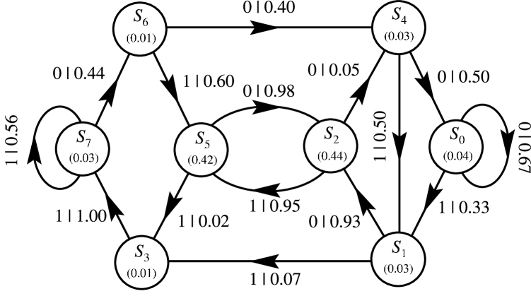
Figure 13: The ${r}=3$ $\epsilon$-machine reconstructed for SK229. The large asymptotic state probabilities for the ${\cal S}_{2}$ and ${\cal S}_{5}$ states, as well as the large state-transition probabilities between them, show that this is predominately a 2H crystal with some faulting.

Structure	Contribution
2H	$82\%$
3C	$4\%$
Deformation fault	$9\%$
Growth fault	$4\%$
Other disorder	$1\%$

Table 2: The Fault Model structural interpretation of the reconstructed $\epsilon$-machine of Fig. 13. This is valid only under the assumption of weak faulting.

SK229 has not been analyzed quantitatively using the FM. By comparing the FWHM of the integer-$l$ to half-integer-$l$ peaks, Sebastian and Krishna Sebastian and Krishna (1994) concluded that deformation faulting is the primary vehicle responsible for the deviation from crystallinity seen here. We are in agreement, except that we also detect small amounts of 3C crystal structure and some growth faults.

Figure 14: Comparison of the $Q_{s}(n)$ versus $n$ for experimental spectrum SK229 (solid squares) and the $\epsilon$-machine (open squares).

Figure 14 compares the CFs from experiment and the $\epsilon$-machine. The agreement is good, although the reconstructed $\epsilon$-machine underestimates somewhat the magnitude of the oscillations in $Q_{s}(n)$. A visual comparison of the experimental diffraction spectrum and that generated from the $\epsilon$-machine (Fig. 12) shows that there is reasonable agreement. We calculate an ${\cal R}$-factor between the two spectra of ${\cal R}_{\epsilon M}=29\%$.

There are some noticeable differences between the two spectra, however. First, we see that Bragg-like peaks in the $\epsilon$-machine spectrum are slightly shifted from those in the experimental spectrum. Second, the $\epsilon$-machine spectrum overestimates the maximum intensity in each peak. Third, the peak profiles are qualitatively different. For the $\epsilon$-machine, the shoulders of the peaks are broader than those of the experiment and the crowns are narrower. Indeed, the peaks in the experimental spectrum appear plateau-like. The sides are very steep and the crown is rounded. It is not known if this results from instrument resolution or it is an observable effect.

This example shows that slightly faulted crystals with sharp Bragg-like structures can be difficult to analyze. Certainly, the basic crystal structure is clear—in this case 2H, but a very fine experimental $l$-mesh is needed to map each Bragg peak. In contrast, highly disordered spectra with significant diffuse scattering are less sensitive to experimental details, such as instrument resolution. For highly diffuse spectra, where the assumptions underlying the FM break down, $\epsilon$MSRboth in practice (extraction of correlation information) and in principle (the $\epsilon$-machine describes any amount of disorder) reaches its full potential.

From the $\epsilon$-machine we calculate the three length parameters to be ${r}=3$ ML, $\mathcal{P}=3.5$ ML, and $\lambda_{c}=19\pm 2$ ML. The three measures of intrinsic computation are found to be ${h_{\mu}}=0.30$ bits/ML, ${C_{\mu}}=1.8$ bits, and ${\bf E}=0.89$ bits.

IV Physics from $\epsilon$-Machines

Now that we have models ($\epsilon$-machines) for the stochastic processes underlying the observed ML stacking for each sample, we can calculate a range of structural, computational, and physical characteristics that describe the stacking patterns and disorder. In Table 3 we list the measures of intrinsic computation and characteristic lengths calculated for each sample, as well as for three crystal structures for comparison.

IV.1 Characteristic Lengths in Polytypes

We first note that it was necessary to perform $\epsilon$MSR up to ${r}=3$ for each spectrum. This is not surprising since the mechanism of deformation faulting is expected to be important in ZnS, and the minimum $\epsilon$-machine on which deformation faulting structure can be modeled is ${r}=3$. This implies, of course, a longer memory length that either pure 3C or 2H structure alone requires. The generalized periods for the 2H and 3C structures at $\mathcal{P}=2$ ML and $\mathcal{P}=1$ ML, respectively, are also much shorter than for the disordered structures which average $\mathcal{P}=5.7$ ML. This shows that there is spatial organization over a modest range—$6$ MLs—for disordered ZnS crystals. This pales in comparison to crystalline polytypes with repeat distances over 100 MLs, but is still much larger than the calculated range of inter-ML interactions of $\sim$ 1 ML. We note that many of these long-period crystalline polytypes are believed to be associated with giant screw dislocations that are expressly absent here. For both ${r}$ and $\mathcal{P}$, the disordered structures have values much closer to that expected for the 6H structure. In contrast to a perfect crystal, the correlation lengths are finite rather than infinite. Interestingly, the sample that has the most stacking disorder (as measured by ${h_{\mu}}$), SK137, also has a comparatively long correlation length. While this was previously classified as an as-grown 3C crystal by Sebastian and Krishna, Sebastian and Krishna (1994) we find that it also contains a significant amount of stacking sequence associated with the 2H structure. Since we cannot assume that any of these structures are in equilibrium or the ground state, we can draw no conclusions about the range of inter-ML interactions.

IV.2 Intrinsic Computation

Each of the diffraction spectra we analyze also show much stacking disorder. Even a spectrum that is quite crystalline, like SK134, has a stacking entropy of ${h_{\mu}}=0.50$ bits/ML. Of course, for a crystal the entropy rate is zero and for the case of completely disordered stacking one would have ${h_{\mu}}=1$ bits/ML. If we compare SK134 and SK135, each beginning as a 2H crystal but annealed at different temperatures, we see that the latter is slightly more disordered, as we expect. The statistical complexity, a measure of the average history in MLs needed to predict the next ML, is also relatively constant at $2.3$ bits and $2.5$ bits, respectively.

In fact, the measures of intrinsic computation are nearly equal, except those for SK229. But SK134 and SK135 have very different structures. SK134 is largely 2H in character while SK135 is largely twinned 3C. Assuming that they were identical before annealing, this would suggest that the disordering process has little effect on these measures. This is, of course, tentative, since such a conclusion can only be drawn after examining many disordered samples. Experimental spectra in the midst of the 2H-to-3C transformation would be of significant interest here. It is possible, though, that SK137 might be such a instance. While this is an as-grown twinned 3C crystal, as noted above this, this crystal also has some significant 2H character. Since Sebastian and Krishna Sebastian and Krishna (1994) found that both of these were well described by a random distribution of twin faults, they concluded that disordered 3C crystals found in the growth furnace result from a phase transformation from the 2H structure upon cooling the furnace. We find that the two samples (SK135 and SK137), while similar, do have qualitative differences. We can understand this either as a crystal not completely transformed or that the mechanism which created SK137 is not simple. We feel that more experimental data is needed in order to arrive at a more complete understanding. Since ${h_{\mu}}=0.65$ bits/ML for SK137 and is thus more disordered than either SK134 or SK135, the interpretation of this crystal being in the midst of a phase transition is a plausible explanation. The most striking feature of the measures of intrinsic computation is their relative consistency (except for SK229) even while the structure of the crystal changes significantly.

System	$\lambda_{c}$	$\mathcal{P}$	${r}_{l}$	${h_{\mu}}$	${C_{\mu}}$	${\bf E}$	$\Delta$
2H	$\infty$	2	1	0	1.0	1.0	0.0
3C	$\infty$	1	0	0	0.0	0.0	0.0
6H	$\infty$	6	3	0	2.6	2.6	0.0
SK134	$9.5\pm 0.5$	4.8	3	0.50	2.3	0.75	-0.1
SK135	$4.4\pm 0.7$	5.6	3	0.59	2.5	0.71	0.0
SK137	$12\pm 3$	6.7	3	0.65	2.7	0.79	0.0
SK229	$19\pm 2$	3.5	3	0.30	1.8	0.89	0.0

Table 3: A comparison of the three characteristic lengths and three measures of intrinsic computation that one can calculate from knowledge of the $\epsilon$-machine. We calculate them for the experimental diffraction spectra, as well as for three crystal structures for reference. Recall that $\Delta={C_{\mu}}-{\bf E}-r{h_{\mu}}$.Varn et al. (2003)

IV.3 Stacking-Fault Energies

One physical quantity amenable to calculation from the $\epsilon$-machine is the difference in configurational energies of the particular polytypes. Numerical calculations find that the configurational energy depends only the nearest and the next-nearest neighbors in the stacking arrangement. Engel and Needs Engel and Needs (1990) have done a first-principles pseudopotential calculation of the total energy of five ZnS polytypes, from which they determined the strength of the interactions up to the third nearest layer. The most general expression possible for inter-ML interactions up the third nearest neighbors is given by Shaw and Heine (1990)

$$E = E_{0}-J_{1}\sum_{i}s_{i}s_{i+1}-J_{2}\sum_{i}s_{i}s_{i+2}$$ (1)

$$-J_{3}\sum_{i}s_{i}s_{i+3}-K\sum_{i}s_{i}s_{i+1}s_{i+2}s_{i+3}~{}.$$

Terms with an odd number of spins do not appear due to symmetry considerations. We take $s_{i}=\pm 1$ here.

Engel and Needs Engel and Needs (1990) found that $J_{1}=0.00187$ eV per ZnS pair and $J_{2}=-0.00008$ eV per ZnS pair and that $J_{3}$ and $K$ are negligible. Given this let us rewrite Eq. (1) in terms of the energy per ZnS pair and take $E_{0}=0$. Then the configurational energy is

$$\tilde{E}=-J_{1}\langle s_{i}s_{i+1}\rangle-J_{2}\langle s_{i}s_{i+2}\rangle~{},$$ (2)

where brackets indicate the expectation value over the stacking sequence. The expectation values are found directly from sequence probabilities, as follows:

$$\langle s_{i}s_{i+1}\rangle = {\rm P}(11)+{\rm P}(00)-2{\rm P}(01)$$

$$\langle s_{i}s_{i+2}\rangle = {\rm P}(111)+{\rm P}(101)+{\rm P}(000)+{\rm P}(010)$$ (3)

$$-2{\rm P}(110)-2{\rm P}(100).$$

The configurational energy in terms of meV per Zn-S pair is shown in Table 4 for several crystalline structures and each of the four disordered samples. The configurational stacking energies are bounded above and below by the 2H and 3C structures with relative configurational energies of 1.95 meV/ZnS-pair and -1.79 meV/ZnS-pair, respectively. For SK134, the annealing process has introduced faults and has lowered the average stacking energy from the original 2H structure to $1.13$ meV/ZnS-pair, while increasing the stacking entropy. If we assume that SK137 is a partially transformed 2H-to-3C crystal (though mostly 3C), then we see that the crystal experiences further disordering and the stacking energy falls to -0.57 meV/ZnS-pair. SK135 shows the most advanced transformation with the 2H structure almost completely eliminated and stacking energy not too far from the ideal minimum at -1.02 meV/ZnS-pair. The stacking entropy begins to fall, however, as the transformation nears a disordered 3C crystal. Being only a slightly disordered 2H crystal, SK229 shows the highest stacking energy of 1.56 meV/ZnS-pair. As we might expect from the relative magnitudes of $J_{1}$ and $J_{2}$, the contribution from the $J_{1}$ term completely dominates the energy.

System	$\langle s_{i}s_{i+1}\rangle$	$\langle s_{i}s_{i+2}\rangle$	$\tilde{E}$	$\alpha_{h}$	History
2H	-1.00	1.00	1.95	1.00	PC
3C	1.00	1.00	-1.79	0.00	PC
6H	0.33	-0.33	-0.65	0.33	PC
SK134	-0.58	0.63	1.13	0.80	D 2H, 300 C for 1h
SK135	0.56	0.45	-1.02	0.24	D 2H, 500 C for 1h
SK137	0.32	0.45	-0.57	0.34	AG 3C
SK229	-0.80	0.86	1.56	0.90	AG 2H

Table 4: Relative configurational energies $\tilde{E}$ of experimental polytypes and several pure-crystalline polytypes. The last column gives the history of each sample, where PC stands for perfect crystal, AG as-grown, and D disordered. We use the energy coupling constants, $J_{1}$ and $J_{2}$, calculated by Engels and Needs along with the reconstructed $\epsilon$-machine for the disordered processes to find the configurational energy of the disordered structures via Eqs. (2) and (3).

IV.4 Hexagonality

The degree of birefringence of ZnS crystals is known to depend only a single structural parameter—the hexagonality $\alpha_{h}$. Brafman and Steinberger (1966) This parameter is defined as that fraction of MLs which are hexagonally related to their neighbors. That is, $\alpha_{h}$ is defined as the frequency of occurrence of sequences $ABA$ and $BAB$ and their cyclic permutations. In terms of the Hägg notation, these are simply ${\rm P}(01)$ and ${\rm P}(10)$, respectively. Since ${\rm P}(01)={\rm P}(10)$, Varn et al. (2003) we have

$$\alpha_{h}=2{\rm P}(01)~{}.$$ (4)

Sequence probabilities are directly calculable from the $\epsilon$-machine, so that the hexagonality of a disordered crystal can be easily found.

In Table 4 we show the hexagonality calculated for all of the spectra, as well as for several crystal structures for comparison.

V Discussion

We have successfully applied computational mechanics to the discovery and description of stacking order in single crystals of polytypic ZnS. In doing so, we reconstructed from experimental diffraction spectra the minimal, optimal, and unique description of the stacking process as embodied in the $\epsilon$-machine. In contrast to previous analyses, Sebastian and Krishna (1994) we used all of the information in the diffraction spectra, both in the Bragg peaks and in the diffuse scattering between them. We imposed no restrictions on the kind of structures to be found, save that they be representable by $\epsilon$-machines. Further, the computational mechanics approach was not limited to the case of weak faulting, but can be used to treat even highly disordered samples. Additionally, the $\epsilon$-machine can naturally accommodate more than one parent crystalline structure as seen in SK134.

For two of the spectra, a sensible decomposition not (c) of the $\epsilon$-machine into crystal and faulting structure was possible, allowing a direct comparison between the computational mechanics approach and the FM. The $\epsilon$-machine detected structures not previously found by the FM. For example, in SK134 we found that not only was structure associated with deformation faulting important, but there was also structure related to growth faults and layer-displacement faulting. We even found nascent sequences leading to the 3C structure. For the other two cases, while no FM-like decomposition of the $\epsilon$-machine was proposed, we still found significant structure as embodied in the $\epsilon$-machine. From the $\epsilon$-machine, physical insight into the structure of the stacking was possible. For example, in the ${r}=3$ reconstructed $\epsilon$-machine for SK137 we could eliminate 6H structure based on the absence of a transition between CSs. We also found that 2H structure was present. Even when no sensible decomposition into a simple pure-crystal and weak-faulting structure is possible, the $\epsilon$-machine still directly provides sequence frequencies, which can be used to build physical insight into the stacking structure.

From a knowledge of the $\epsilon$-machine, it is possible to calculate a number of physical characteristics. In Table 4 we tabulated the stacking entropy per ML for each spectrum. Given the coupling parameters between MLs we calculated the average stacking-fault energy for the samples, as shown in Table 4. We were also able to find the hexagonality for the disordered crystals. Knowing the $\epsilon$-machine allowed us to find various characteristic lengths associated with each disordered crystal, such as the memory length and the generalized period. We believe that additional physics can be calculated from the $\epsilon$-machine.

We also calculated measures of intrinsic computation from the $\epsilon$-machine. We found that the minimum memory length for all samples was ${r}=3$, which is in excess of the calculated inter-ML interaction range of $\sim 1$ ML for ZnS. We further found that the statistical complexity, a measure of the amount of information in the $\epsilon$-machine, was also much larger than that of either the pure 2H or 3C structures. Also, the range over which structures are found in the disordered samples is about 6 ML.

Characterizing solid-state transitions in polytypic materials is of considerable interest. Let us review what an $\epsilon$-machine does and does not imply. Most simply put, the $\epsilon$-machine is the answer to the question, What is the minimal, optimal, and unique description of the one-dimensional stacking structure of the sample?Any physical parameters that depend on this description are in principle calculable from $\epsilon$-machine. The $\epsilon$-machine does not answer the question, How did the crystal come to be stacked in this way? To determine this, one must augment structural knowledge (as embodied in the $\epsilon$-machine) with additional information or assumptions. Such information can come in the form of a time series of structures obtained either from a series of numerical simulations or experiments or, in the theoretical domain, perhaps from assumptions about weak faulting.

Since we have discovered structures in polytypic ZnS that were undetected before, we feel that the mechanism of faulting—previously attributed to deformation faulting—deserves re-examination. We have provided a firm theoretical foundation for the discovery and description of disordered stacking sequences in polytypes and believe that additional experimental studies are warranted. Additionally, computer simulations of solid-state transformations in polytypes with proposed faulting mechanisms, accompanied by the concomitant reconstruction of the $\epsilon$-machine directly from the sequence of MLs from the simulation, should provide a powerful method to understand the gross features of the transformations.

Before such studies can be definitive, a quantitative understanding of the effects of experimental error on the reconstructed $\epsilon$-machine is needed. With the exception of our introduction of the figures-of-merit, $\gamma$ and $\beta$, we have not addressed this important issue here. We note that the original experimental data was not reported with error bars and this means that comparison with the desired $\epsilon$-machine error analysis would have not been possible. Additionally, the necessity to digitize the data undoubtedly introduced errors. It is therefore difficult to assess the amount of error in each spectrum. Our intuition tells us that error in the diffraction spectrum will likely lead to suppression of the more delicate structures on an $\epsilon$-machine. Therefore, one should expect to find less structure and more randomness.

We mention that the application of computational mechanics to the description of one-dimensional sequences is the most general approach possible to this problem. Thus, its application here to polytypism represents the end point in the evolution of models to describe the disordered sequences seen these substances. Any alternate description can be expressed as an equivalent $\epsilon$-machine and none can be more general, since in the language of statistics an $\epsilon$-machine is the minimal sufficient statistic for the underlying process. It may be possible to find specialized algorithms that are more sensitive or more efficient in determining an $\epsilon$-machine than the one we introduced in $\epsilon$-machine spectral reconstruction. However, the answer, in its most general form, will be expressible as an $\epsilon$-machine.

We also note that our work here represents a solution to a significant theoretical problem—How does one extract structural information from a power spectrum? Our application has been to polytypism, but the principles underlying our solution may be applied quite generally to domains in which spectral information is available.

Future directions for this work include an application of $\epsilon$MSR to other polytypes, as well as to substantially more complex materials. The extension of these ideas to the more common cases of disorder in two and three dimensions is also desirable. The development of computational mechanics in higher dimensions would significantly aid in the classification and understanding of disorder in many physical systems.