Exploring Valleys of Aging Systems: The Spin Glass Case

Abstract

We present a statistical method for complex energy landscape exploration which provides information on the metastable states—or valleys—actually explored by an unperturbed aging process following a quench. Energy fluctuations of record size are identified as the events which move the system from one valley to the next. This allows for a semi-analytical description in terms of log-Poisson statistics, whose main features are briefly explained. The bulk of the paper is devoted to thorough investigations of Ising spin glasses with Gaussian interactions of both short and long range, a well established paradigm for glassy dynamics. Simple scaling expressions with universal exponents for (a) barrier energies, (b) energy minima, and (c) the Hamming distance as a function of the valley index are found. The distribution of residence time inside valleys entered at age $t_{w}$ is investigated, along with the distribution of time at which the global minimum inside a valley is hit. Finally, the correlations between the minima of the landscape are presented.

The results fit well into the framework of available knowledge about spin glass aging. At the same time they support a novel interpretation of thermal relaxation in complex landscapes with multiple metastable states. The marginal stability of the attractors selected is emphasized and explained in terms of geometrical properties of the landscape.

I Introduction

Physical properties of glassy systems quenched from a high temperature slowly change with the time or age $t_{w}$ elapsed since the quench. For any $t_{w}$ well below the true equilibration time, the dynamics deceptively appears to be stationary when observed on time scales shorter than $t_{w}$. Experimental and numerical evidence for the presence of a quasi-stationary fluctuations regime for $t\ll t_{w}$ followed by non-equilibrium drift for $t\gg t_{w}$, stems e.g. from measurements of conjugate linear response and autocorrelation functions Reim86 ; Refrigier87c ; Andersson92 which obey, respectively violate, the fluctuation-dissipation theorem in the two regimes. In general, the (apparent) age of the system can be deduced from the decrease in the rate of change of macroscopic averages. This apparent age can however be ‘reset’ to an earlier value by applying a perturbation of short duration, as e.g. a temperature pulse, which thus rejuvenates the system.

Non-equilibrium memory effects such as aging and rejuvenation were first noticed and studied in a spin glass context Granberg88 ; Granberg90 ; Schultze91 ; Hoffmann97 , but are now observed in a variety of glassy systems Kityk02 ; Nicodemi01 ; Sibani01 ; Bureau02 ; Hannemann02 . Expanding a previous brief exposition sibani02a , we describe and test a statistical approach to landscape explorations designed to find the generic properties of the energy landscape which produce these effects.

Our main point is that the dynamical events marking the transition between the quasi-equilibrium and the off-equilibrium dynamical regimes are triggered by the attainment of energy values of record magnitude. This immediately allows a description of the non-equilibrium dynamics in terms of a log-Poisson process Sibani93a ; sibanidall03a , i.e. a stochastic process which is homogeneous when viewed on a logarithmic time scale.

The sequel is organized as follows: the next section introduces the landscape exploration method. Section III briefly explains the relevant properties of the log-Poisson statistics used throughout the paper as a semi-analytical description of non-equilibrium dynamics. Section V presents results of an extensive application of the method to spin glass systems, demonstrating the viability of the method and the usefulness of the log-Poisson description. Section VI puts the results in a broader perspective, with special reference to coarse-grained mesoscopic models of configuration space. In particular, we discuss the connection between aging in thermalizing systems and in dissipative driven system and biological evolution. Section VII is a summary and an outlook.

As the nature of true equilibrium and the final stages of thermal relaxation are only weakly related to the presented data, no theoretical consideration is given to these aspects in the paper.

II The Method

In models of driven dissipative systems with multiple attractors Sibani01 ; Sibani93a ; Coppersmith87 , marginally metastable attractors with an a priori negligible statistical weight are nevertheless those typically selected by the dynamics. In such systems, this mechanism underlies memory and rejuvenation effects analogous to those observed in the thermalization of e.g. spin glasses Jonason98 after a quench. One can speculate that similar mechanisms could generally be present in glassy systems with an extensive number of metastable attractors. However, the issue of attractor selection is not explicitly considered in widely used landscape exploration methods such as the Stillinger-Weber approach Stillinger83 ; Nemoto88 ; Becker97 ; Crisanti02 ; Mossa02 , which study a set of local energy minima (inherent states) generated by quenches. The same applies to exhaustive landscape exploration techniques Sibani93 ; Sibani98 ; Schon96 and studies of the real space morphology of low-energy excitations by techniques requiring quenches Andersson96 , genetic algorithms Palassini99 and energy minimization of excitations of fixed volume Houdayer00 ; Lamarcq02 .

The ability of small external perturbations to induce strong rejuvenation and memory effects in complex dynamics strongly suggests that any probe introducing extraneous elements in the dynamical evolution might at the same time yield a biased picture of the energy landscape. In other words: are the attractors identified also those which would be selected by e.g. the unperturbed thermalization process after a deep quench or any other dynamical evolution of interest? Analyzing the regions of state space surrounding intrinsic states provides valuable information about the quasi-equilibrium (fluctuation) dynamics in the energy landscape, but it does not tell the whole story. The question of how to properly describe the non-equilibrium process of ‘selecting’ the metastable states is still open. This question motivates the present approach which is based solely on statistical information collected during an undisturbed aging process.

Conventionally, a valley is a connected neighborhood of configuration space which supports a state of approximate thermal equilibrium centered on a local energy minimum. During the time a trajectory ‘resides’ in a valley, the energy and other physical quantities fluctuate around a fixed average, and the state of lowest energy is often revisited; the dynamics has a recurrent character. Non-equilibrium events, henceforth ‘quakes’, move the system irreversibly from the neighborhood of the initial local energy minima of high value and into progressively deeper valleys. A sequence of such events seldom or never revisits the same configurations and has a transient character.

As widely recognized, the lack of time translational invariance in aging systems stems from the dynamical in-equivalence of the valleys visited. Consider therefore a landscape with multiple valleys of varying degrees of metastability, or depth. On time scales larger than the residence time of the deepest (i.e. most stable) valley seen up to the age $t$, all valleys shallower than this valley are, by definition, unstable and hence irrelevant for the non-equilibrium dynamics. The interesting dynamical objects are thus the valleys deeper than the deepest valley seen up to time $t$. This points to energy records as prospective markers of the non-equilibrium events.

We shall use the term ‘energy barrier’ to denote the difference between the energy of the current state and the lowest seen or best-so-far energy minimum. The lowest energy minimum value and the highest energy barrier observed up to time $t$ will identify the valleys as they successively appear in the landscape.

Our classification procedure of the undisturbed dynamics is as follows: We save the minima and barriers of record values encountered and the times at which they occur. We stipulate that a valley is entered at time $t$ if the barrier record achieved at time $t$ happens to be the last one prior to the attainment of a energy minimum record. To leave a valley, a barrier record must again be followed by a record in the lowest energy. Whenever several minima records are found between two barrier records, we only keep the latest, and therefore deepest, minimum.

In short, we operationally identify the valleys encountered by a series of minima records with at least one barrier event between them. Note that this selection procedure must be performed retrospectively, since it is impossible to know ‘on the fly’ whether a new valley has been entered or not. We also stress that the barrier records will not necessarily coincide with the lowest barrier separating two consecutive energy minima records, as the dynamics, due to entropic effects, is not likely to follow the path of lowest energy, an effect noticed by Wevers et al. Wevers99 in the landscape of metastable ionic compounds.

The discovery of a new record in low energy is a non-equilibrium event. However, by no means does it imply that the internal dynamics in a valley is entirely equilibrium-like. Several sub-valleys are typically explored before the energy minimum is encountered which eventually remains as the lowest state within the valley. Only then does the dynamics acquire the recurrent, fluctuation-like nature which is characteristic of quasi-equilibrium.

Resetting the highest barrier to zero at an arbitrary point in time produces numerous barrier records but no new valleys before a lower energy value is again recorded. However, resetting both the record energy and barrier values to zero may result in a series of new records being registered, which describe sub-valleys within the valley originally explored. By repeating the simulation with the exact same random numbers, this procedure allows one to take a closer look at the internal structure of a valley if the resetting is done at the time of entry.

The method presented is generally applicable, easily implemented, and does not add much to the total runtime of a simulation. If the energy landscape explored is simple, e.g. if it contains one large, structureless valley or if it is perfectly periodic, our scheme only detects a single valley, since degenerate and hence dynamically equivalent minima are appropriately lumped together. In other words, our method produces simple results when used on simple systems. In the following sections we show that non-trivial results are indeed the outcome when complex landscapes are explored.

III Log-Poisson statistics

In this section we introduce and motivate the log-Poisson statistics used through the paper as an idealized analytical description of non-equilibrium events—such as the quakes which lead to new valleys. We mainly focus on the consequences and predictions for various quantities of physical interest, leaving the empirical justification of the formalism to the next section, where the data are also presented.

A log-Poisson description of complex dynamics was first introduced in connection with a model of Charge Density Waves Sibani93a , and later used to explain macro-evolutionary patterns from the fossil record Sibani95 ; Sibani98a . It describes Sibani99a the coarse grained dynamics of a population evolving in a NK landscape Kauffman87 , and there are indications that it might also apply to far more realistic models of evolution Hall02 .

The familiar Poisson process with the time argument replaced by its logarithm is in short denoted log-Poisson:

$$P_{k}(t)=\frac{(\alpha\ln t)^{k}}{k!}t^{-\alpha},\ \ t\geq 1.$$ (1)

As shown in Sibani93a ; Sibani98a , the probability that $k$ records occur in a sequence of $t$ random numbers is given by Eq. (1), independently of the underlying process generating the numbers. Log-Poisson statistics implies that the tempo at which the events occur falls off as $1/t$. Switching to $\log t$ as the independent variable gives a constant (logarithmic) rate of events, and restores time homogeneity. Several other interesting mathematical properties of log-Poisson processes are listed below together with their physical implications for the spin glass problem at hand.

The probability that $k$ ‘events’ occur between $t_{w}$ and $t_{w}+t$ is sibanidall03a

$$P_{k}(t_{w},t_{w}+t)=\frac{1}{k!}\left[\alpha\ln\left(\frac{t_{w}+t}{t_{w}}\right)\right]^{k}\left[\frac{t_{w}+t}{t_{w}}\right]^{-\alpha}.$$ (2)

Consider a function $c(m,m+k)$ describing the effect of $k$ events, for example the overlap between the configurations of lowest energy in valleys $m$ and $m+k$. To connect with the thermal correlation $C(t_{w},t_{w}+t)$, we can utilize a cartoon rendering of the coarse-grained non-equilibrium dynamics as a one dimensional walk on a set of states corresponding to the minima of the valleys, which is similar to e.g. one of the basic assumptions of Ref. rinn00 . We assume, in our terminology, that the dynamical trajectories of an aging system dwell at the bottom of the ‘current’ valley for a certain residence time, until a quake instantaneously moves them to the bottom of the next valley. This coarse grained picture neglects the internal structure of the valleys, which is questionable since the time spent searching for the bottom state within a valley is of the same order of magnitude as the full residence time, see e.g. Fig. 7. Nevertheless, the cartoon has the virtue of simplicity, and allows us to write

$$C(t_{w},t_{w}+t)=\sum_{m,k}P_{m}(t_{w})P_{k}(t_{w},t_{w}+t)c(m,m+k).$$ (3)

which is a function of $t/t_{w}$ if and only if $c(m,m+k)$ is independent of $m$. This pure or full aging form has very recently been shown to describe aging in real spin glasses, if cooling rate effects through the critical temperature are accounted for rodriguez02 . The assumption that $c(m,m+k)$ only depends on a single argument has been checked separately, and an additional dependence on the valley index $m$ has been found, which entails a deviation from $t/t_{w}$ scaling dall03b for the numerical models.

For later convenience we finally note that, if $t_{k}$ marks the time of the $k$’th event in a log-Poisson process occurring after $t$, the ‘log-waiting time’ $\log(t_{k})-\log(t)$ is exponentially distributed, in perfect analogy to the usual Poisson process. The same exponential distribution also describes the series of independent variables $\log(t_{k})-\log(t_{k-1})$. This property of the log-waiting time distribution is very well fulfilled by our data.

IV Models and Dynamics

As glassy dynamics is insensitive to many details of the interactions, computational convenience is a prime criterion for choosing a test model. Spin glass models are comparatively easy to simulate and have been investigated experimentally and numerically for more than twenty years. The lack of a comprehensive and coherent picture of their dynamics and statics furthermore endows them with considerable intrinsic interest.

This section demonstrates that a simple and consistent geometrical picture of the spin glass energy landscape is obtained with our ‘non-invasive’ exploration method. Current spin glass issues are mentioned as needed, while a more complete discussion can be found in Section VI.

We consider $N$ Ising spins, where the energy of a spin configuration $\mathbf{s}=\{s_{1},\ldots,s_{N}\}$ is given by

$$E(\mathbf{s})=-\frac{1}{2}\sum_{i,j}J_{ij}s_{i}s_{j},$$ (4)

where the couplings $J_{ij}$ are symmetric, independent Gaussian variables of unit variance. To test the importance of the topology of the system, we have simulated lattices with periodic boundary conditions in both $2d$, $3d$ and $4d$ ($N=L^{d}$), where $J_{ij}$ are non-zero only if $i$ and $j$ are lattice neighbors. Additionally, we have placed the spins in a $k$-regular random graph, i.e. each spin interacts with exactly $k$ spins chosen at random.

We use single spin flip dynamics coupled with a rejectionless algorithm, the Waiting Time Method Dall01 . The latter generates a sequence of moves equal in probability to the sequence of accepted moves in the Metropolis algorithm. Thus, the results of this paper can also be obtained with the standard Metropolis algorithm, albeit at the price of considerably longer run times. The ‘intrinsic’ and size independent time variable $t$ used throughout corresponds to the number of Monte Carlo (lattice) sweeps in the Metropolis as well as to the physical time of a real experiment. We refer to Dall01 for a detailed account of the Waiting Time Method. In all our runs, we conventionally skip the data within the first $10$ time units in order to let the system settle down from the random $T=\infty$ initial configuration.

V Results

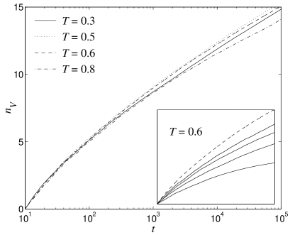
Figure 1: The average number of valleys $\overline{n_{V}}$ visited as a function of time in $3d$ Gaussian spin glasses with $N=16^{3}$ spins. For $t>100$ a curvature is barely discernible. The insert shows $\overline{n_{V}}$ for system sizes $L=6,8,10$ and $12$ (full lines), as well as $L=16$ (dashed line as in the main panel).

Figure 1 shows the average number of valleys $\overline{n_{V}}(t)$ (which is equal to the number of quakes leading from a valley to another) observed in $3d$ at various low temperatures. Neglecting the earliest part of the simulations where the memory of the initial random spin configuration is still present, $\overline{n_{V}}(t)$ has a logarithmic shape. As the ratio of the variance $\sigma^{2}_{n_{V}}(t)$ to $\overline{n_{V}}(t)$ is constant and close to one (see Fig. 2 of ref. sibanidall03a ), the statistics of valleys is essentially a $\log$-Poisson process, as expected in a record induced dynamics Sibani93a . As this holds true for barrier records as well (not shown), the ratio of the number of barrier records to minima records is therefore constant on average. This non-trivial geometrical feature of the spin glass landscape has not previously been noted, and it provides a link to an analytical description of the non-equilibrium dynamics as a log-Poisson process Sibani93a ; sibanidall03a .

The barely perceptible curvature seen in Fig. 1 for large $t$ decreases systematically as the system size increases at a fixed temperature, as shown in the insert. The sub-logarithmic form of $\overline{n_{V}}(t)$ means that the likelihood that a record in low energy follows a barrier record decreases very slowly, but systematically as the system ages. Taking into consideration that the curvature seems to vanish in the limit of a very large system (see Fig. 2 of ref. sibani02a , which shows that the slope of the straight part of $\overline{n_{V}}(t)$ seems to be proportional to $\log(N)$), we surmise that its presence reflects the increasing difficulty in finding new low energies as the ground state is approached.

In summary, the series of quakes moving the system from one valley to the next can be meaningfully idealized into a log-Poisson process discussed in the previous section, if one disregards the curvature of the data. How record events are distributed in time is insensitive to the properties of the stochastic process from which the records are drawn Sibani93a . In our case Figs. 1 and 5 have a weak temperature dependence, as opposed to the strong $T$ dependence of the underlying fluctuations. Finally, we note that identical results with respect to $\overline{n_{V}}(t)$ are also found in $2d$, $4d$ and random graphs.

The rest of this section deals with two scaling plots similar to those presented in ref. sibani02a (Figs. 2 and 4), as well as new results concerning the scaling of Hamming distances (Fig. 3) between the local minima of contiguous valleys. Finally, the statistics of the residence time and the fraction thereof spent before hitting the lowest energy state in the valley is analyzed, along with the correlations between the minima of the valleys.

V.1 Scaling of barriers

The data shown in this section are averages over many thousands of realizations of the couplings $J_{ij}$ and cover a wide range of low temperatures and system sizes. The raw data for each $T$ and $N$ have very little scatter, and the main sources of error are systematic. For example, our finite runtimes of $t=10^{6}$, combined with the very broad distribution of residence times in the valleys, bias the average energy of valleys discovered late in the process, since only the ’faster’ trajectories are able to explore these. The data are parametrized by the valley index $i$.

In our plots the scaling of the ordinate is given in the corresponding labels. The value of the valley index $i$ is shifted from one data set to another by up to one unit. This corresponds to a multiplicative shift of the age, and compensates for the arbitrariness of skipping data within the first 10 time units after the quench, irrespective of temperature and system size.

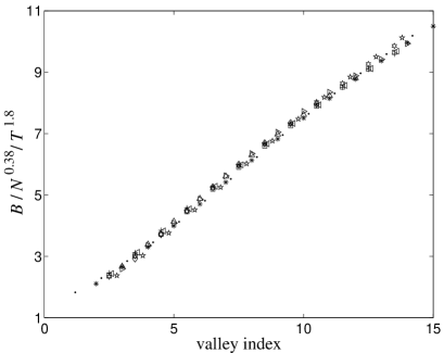
Figure 2: Average energy barrier records $B$ separating contiguous valleys in random graph spin glass landscapes are scaled with system size $N$ and temperature $T$ as indicated in the ordinate label and plotted versus the valley index. The data points are based on $N=4096$ and $T=0.3,...,0.7$ as well as $T=0.5$ and $N=1000,...,16000$. The same scaling form $B\sim N^{0.38}T^{1.8}$ applies equally well to our $2d$, $3d$, and $4d$ data.

Figure 2 is a scaling plot of the energy barrier $B_{i}$ which on average must be surmounted in order to leave the $i$’th valley. The system is a $k$-regular random graph with $k=6$, i.e. the same number of links per spin as in $3d$. $B_{i}$ is seen to scale in a simple way with the temperature and the size of the system: $B_{i}(N,T)=B_{i}(N^{a}T^{b})$, where $a=0.38(2)$ and $b=1.8(1)$. Interestingly, the very same values of $a$ and $b$ are found when scaling the barrier heights in $2d$, $3d$ and $4d$ lattices as well (see e.g. Fig. 3 in ref. sibani02a ). So, in addition to the non trivial fact that a straightforward two parameter fit works very well, the values of the scaling exponents seem universal. As the next section will reveal, this universality is also found when looking at energy minima and the Hamming distance between them.

The close to linear shape of the scaling plot shows that the barrier heights between valleys gradually increase. Again, we stress that the barriers discussed are those found along an unperturbed trajectory, end hence unlikely to be the lowest barriers between energy minima in contiguous valleys.

Since the exponent $a$ is positive, the quakes do not remain localized to a finite set of spins in the macroscopic limit. Some information on the size and shape of the quakes can be inferred from the scaling law for the energy barrier, if we assume that quakes correspond to the motion through the system of a generalized domain wall. Letting $m$ be the number of spins typically involved in a quake, we write $B\propto m^{x}$ for some exponent $x>0$. Were the barrier energy the outcome of a fluctuation, i.e. the sum of $m$ contributions of random sign, the behavior would be diffusion-like, with $x=1/2$. However, since the barrier crossing process favors low-energy states, we expect a lower barrier energy, i.e. $x<1/2$. As $m\propto N^{0.38/x}$ and $m\leq N$, we conclude that $x\in[0.38,0.5]$. In summary, quakes have a fractal shape with exponent $0.38/x$, and are more space filling than a conventional domain wall in $d\leq 4$.

An explanation of the strongly non-Arrhenius $T$ dependence of the exponent $b$ involves entropic effects and the connection between the quasi-equilibrium dynamics in configuration space and in real space. The qualitative argument given below predicts that the barriers grow linearly with the valley index, and that $b=2$ which is close to the actual value of $b=1.8$. The discrepancy might arise because we neglect that domain sizes are distributed quantities.

In real space, the relevant objects are connected domains Andersson96 ; kisker96 of thermally equilibrated spins which slowly grow in a sea of frozen spins reaching, on average, a linear length scale $\ell(t)$ on a time scale $t$. In the progressively longer quiescent periods between the quakes, these domains do not interact, and their quasi-equilibrium properties are therefore determined by the local density of states ${\cal D}(E)$ pertaining to the configurations accessible to the spins constituting each domain. ${\cal D}(E)$ has been investigated by means of the lid-algorithm Sibani93 for a number of different glassy systems Sibani98 ; Sibani94 ; Sibani99 ; Schon98 ; Schon00 , and has consistently been found to have a close to exponential shape: ${\cal D}(E)\approx\exp(E/T_{0}(\ell))$. The energy scale $T_{0}(\ell)$ is an upper bound for the temperature at which metastability can hold and decreases monotonically with the linear size of the system considered Sibani98 . While the results quoted pertain to systems of fixed size and shape, preliminary investigations confirm that the same behavior applies to spin domains of size $\ell(t)$ which grow within a large system. In this case $T_{0}(\ell)$ becomes a slowly decreasing function of time through the time dependence of $\ell(t)$, and asymptotically approaches $T$ from above. We anticipate that the marginal stability of the valley visited implies that a domain is typically close to its maximal size, i.e. $T_{0}(\ell(t))\approx T$.

Returning to $B_{i}$, we recall that energy barriers delimiting valleys are extremal values in a series of ${\cal O}(t)$ independent outcomes in a system of age $t$, and that each attempt sees energy $E$ with probability

$$P_{eq}(E)\approx\exp\left(-E\frac{T_{0}-T}{T_{0}T}\right).$$ (5)

It follows Leadbetter83 that the typical energy barrier scales as

$$B\propto\frac{T_{0}T}{T_{0}-T}\log t.$$ (6)

Since the valley index grows linearly with $\log t$, the linear dependence on the valley index seen in Fig. 2 is recovered. Finally, since $T_{0}\approx T+\epsilon$ for some small $\epsilon$, one obtains $b\approx 2$ as anticipated.

V.2 Scaling of Hamming distances and energies

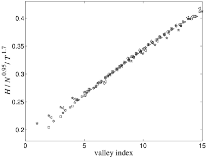
Figure 3: The average Hamming distance $H$ between the lowest energy configurations of two contiguous valleys in $3d$ spin glasses is plotted as a function of the valley index. Combinations of $T=0.5$ and $L=8,10,13,16,20,30,40$ as well as $L=16$ and $T=0.4,...,0.8$ are included. Again, the scaling exponents of $N$ and $T$ are independent of the topology of the networks.

The fact that contiguous valleys contain rather different low energy configurations is shown in Fig. 3, which depicts the scaling of the Hamming distance $H$ (number of spins which differ in their orientation) separating the configurations of lowest energy at the bottom of the two valleys in $3d$ lattices. Again, a simple scaling relation of the kind $H_{i}(N,T)=H_{i}(N^{a}T^{b})$ is found in the $d$-dimensional lattices simulated as well as in regular graphs. The value of $a=0.95(2)$ holds universally, and it indicates that the number of spins involved is more or less an extensive quantity. The temperature exponent $b$ seems to depend slightly on the topology; it has a slightly different value for very low temperatures such as $T=0.3$. In short, near-perfect data collapse does not seem possible for the whole range of low temperatures simulated.

We must emphasize that data for large values of the valley index must be interpreted cautiously when scaling the quantities in Figs. 2–4: Since some runs only reach a few valleys, averages for larger valley indices become biased. This seems particularly important when looking at Hamming distances. Thus, we only plot data for valleys reached by at least $95\%$ of all runs. By lowering this threshold to, say, $80\%$, one will clearly see that the extra data points lie below the master curve.

The strong temperature dependence of $H$ in Fig. 3 is remarkable considering that the energies of the states involved are virtually independent of temperature, as implied by Fig. 4 and as one would expect for actual minima. It follows that the observed minima are nearly degenerate, which is also expected in spin glasses. The $T$ dependence of $H$ is likely due to the fact that at higher $T$ the barriers overcome are higher, and hence the number $m$ of spins involved in a quake is larger. In the simplest scenario where the ‘downhill’ part of the quake does not substantially change $m$, one can assume $m\propto H\propto N^{0.95}$. The energy of the barrier state, which scales as $B\propto N^{0.38}$, must be carried by these $m$ spins. With $B\propto m^{x}\propto N^{0.95x}$, we find $x\approx 0.38/0.95=0.4$, in agreement with the considerations in the previous section.

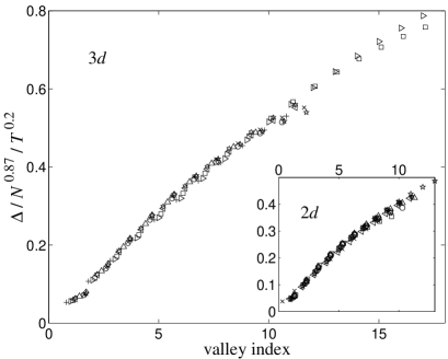
Figure 4: The average difference $\Delta$ between the states of lowest energy found in the first and the $i$’th valley is plotted versus $i$. The data for $3d$ systems is presented in the main panel, where the combinations of $L$ and $T$ shown are as in Fig. 3. The insert shows that the same scaling exponents work equally well in $2d$, where combinations of $T=0.4$ and $L=30,...,100$ as well as $L=64$ and $T=0.2,...,0.7$ are plotted.

The energy difference $\Delta_{i}$ between the state of lowest energy in the first and the $i$’th valley is plotted in Fig. 4 for $2d$ and $3d$ lattices. $\Delta_{i}(N,T)=\Delta_{i}(N^{a}T^{b})$ produces a nice data collapse, with $a=0.87(3)$ and $b=0.2(1)$. Again, these exponents are found in all topologies simulated, as emphasized by the $2d$ data in the insert. The $2d$ data bends slightly more than the $3d$ data in the main panel, preventing the ultimate data collapse. This is true in general of Figs. 2–4: although the same scaling form holds across $2d$, $3d$, $4d$, and $k$-regular random graphs, they have slightly different curvatures.

The linear trend in Fig. 4 means that the lowest energy decreases (almost) logarithmically with the age, a feature already implicit in the early investigations by Grest et al. Grest86 . It also implies that the energy difference between neighboring valleys remains approximately constant along a trajectory. This means that the energy ‘gain’ induced by a quake per participating spin is of order $N^{0.87}/N^{0.95}\approx{\cal O}(1)$ for the range of system sizes investigated. In other words, the height of the barrier which must be overcome to enter a new valley as well as the overlap between them depend strongly on the temperature, while the amount of energy gained is nearly independent of $T$. Hence, lowering the temperature only slows down the process of finding similar valleys. Finally, we mention that the starting point $E_{1}$ when measuring $\Delta_{i}$ is only slightly $T$-dependent. If this was not the case, we could not claim the similarity of valleys as stated above.

To sum up, the plots of Figs. 2–4 tell us that barriers, Hamming distances, and energies of the minima of the valleys can all be scaled with respect to size and temperature in a simple way. Furthermore, the scaling exponents are universal; the same values of the latter are found in $d$-dimensional euclidean lattices as well as in regular random graphs.

V.3 Residence time distribution and superaging

The distribution of time spent in ‘traps’ or valleys of the energy landscape has, to the best of our knowledge, never been measured by others in simulations of spin glass models. The assumed form of this residence time distribution enters heuristic scenarios of spin glass relaxation Bouchaud92 ; Vincent95 , as well as the log-Poisson description of non-equilibrium relaxation sibanidall03a ; dall03b .

Thus, we consider the probability $R(t\mid t_{w})$ that the residence time $t_{r}$ in a valley entered at age $t_{w}$ be less than $t$. As with the scaling plots in the previous sections, a clear picture emerges which lends support to the usefulness of the method for identifying valleys described in Section II.

Before we discuss the numerical results in any detail, we present some theoretical remarks on its expected form for a log-Poisson process. Assuming a pure log-Poisson process for $t_{w}>1$, the ‘log waiting time’ $\ln(t_{r}+t_{w})-\ln(t_{w})$ is exponentially distributed with average $1/\alpha$, where $\alpha=d\overline{n_{V}}/d\ln t$ is the logarithmic slope of the curves in Fig. 1. For any $x>0$, the probability of $t_{r}>t_{w}(e^{x}-1)$ is therefore $e^{-\alpha x}$. Taking $t=e^{x}-1$, the age-scaled residence time probability distribution is

$$R(t\mid t_{w})=1-\left(\frac{t_{w}+t}{t_{w}}\right)^{-\alpha}.$$ (7)

This results also follows directly from Eq. (2) by noting that $R(t\mid t_{w})=1-P_{0}(t_{w},t_{w}+t)$. Since $\alpha>1$ sibanidall03a , the distribution has the finite average $\langle t_{r}\rangle=t_{w}/(\alpha-1)$. Equation (7) has been shown to fit the empirical residence remarkably well sibanidall03a .

The $t/t_{w}$ scaling form is often called pure aging, as opposed to super- or sub-aging where the scaled variable is $t/t_{w}^{\mu}$, with $\mu>1$ or $\mu<1$, respectively. Beside Fig. 5, superaging of the thermal correlation $C(t_{w},t_{w}+t)$ has been observed in numerical investigations of spin glasses berthier02 , while most experimental data show sub-aging vincent97 ; bouchaud99 . Very recent experimental work rodriguez02 shows that subaging is a consequence of the finiteness of the cooling rate. In the limit of a large cooling rate $\mu$ approaches one and pure aging is obtained.

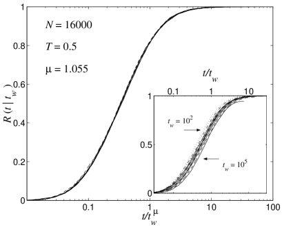
Figure 5: The main panel shows the probability that the residence time $t_{r}$ is less than $t$ for valleys entered at $t_{w}$ for a broad range of $t_{w}$. The abscissa is the scaled variable $t/t_{w}^{\mu}$. The insert shows that the pure aging $t/t_{w}$ scaling predicted by log-Poisson statistics is a fair but far less satisfactory approximation. The system is a spin glass on a $k$-regular random graph with $k=6$.

The empirical data of Fig. 5 are for random graphs of $N=16000$ spins at $T=0.5$. As with all the scaling plots presented so far, the quality of the fit is equally convincing in $d$-dimensional lattices. To study the age dependence of $R(t\mid t_{w})$, the valleys entered are analyzed separately for a broad range of waiting time $t_{w}=10^{2},...,10^{5}$. As the insert shows, a $t/t_{w}$ scaling is a fair approximation, neglecting the small but systematic drift to the right as $t_{w}$ grows.

The main panel reveals that an excellent data collapse can be obtained with

$$R(t\mid t_{w})=R(t/t_{w}^{\mu}),$$ (8)

where $\mu=1.055$. The growth of the residence time with $t_{w}^{\mu}$ shows that the valleys explored become more stable as the system grows older, which concurs with the growth law for the barriers given in Fig. 2. Physically, this means that, compared to the idealized log-Poisson case, the residence time in a valley grows even faster than the age. This deviation from log-time homogeneity is likely due to the already mentioned fact that it becomes relatively harder to find a new valley as the ground state is approached dall03b .

Allowing $\mu$ to depend on $T$, the scaling works well for all temperatures up to $T=0.8$. $d\mu/dT>0$ is observed dall03b , i.e. the superaging effect becomes more pronounced as $T$ increases. Noting that simulations slightly below the critical temperature, i.e. at the high end of the low temperature phase, are able to explore lower energy regions in the same span of time, this strengthens our hypothesis that deviations from $t/t_{w}$ scaling are a reverberation of the finiteness of the ground state energy. As such, these deviations can be expected to become less important the larger the system is, as they indeed do dall03b .

V.4 Correlations

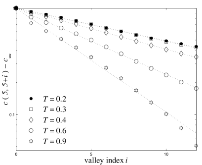
Figure 6: The correlation between the valleys $m$ and $m+k$ for $m=5$ in $4d$ euclidean lattices of size $N=8^{4}$. The decay is clearly exponential for low $T$. Again, this is observed in all topologies tested.

We have investigated the overlap between configurations $m$ and $m+k$ for $m\leq 5$ and $k\leq 12$ and found that the form

$$c(m,m+k)=c_{\infty}(m)+(1-c_{\infty}(m))e^{-\gamma(m)k}$$ (9)

fits the data for our range of low temperatures in euclidean lattices as well as in random regular graphs. Only in $2d$ do we find significant deviations, as expected considering that the aging is interrupted in this case kisker96 . As an example, Fig. 6 shows $c(5,5+k)$ in $4d$ models. A similar plot for $c(1,1+k)$ in $3d$ systems can be found in Fig. 4 of Ref. sibanidall03a , where the connection to the experimentally available non-equilibrium exponent $\lambda$ is verified.

If the limiting value for $k\rightarrow\infty$ of $c(m,m+k)$, $c_{\infty}(m)$, were independent of $m$, it would coincide with the Edwards-Anderson order parameter. Empirically, we find a small $m$ dependence, for which we have no physical interpretation. The exponent $\gamma$ also has a small and almost linear $m$ dependence. As Eq. (9) remains a heuristic approximation of limited value, we have not pursued the size and temperature dependence of the parameters involved in Eq. (9). Still, we find it interesting that a simple exponential parametrization in the number of quakes $k$ accurately describes the data.

V.5 Hitting time for the minima

Having argued that our method of partitioning the sampled states into valleys leads to consistent results and provides useful insight into the coarse structure of complex energy landscapes, it is natural to take a first look at the rich internal structure of the valleys. The existence of such a structure is implied by the wide distribution of residence times, which requires a matching distribution of internal energy barriers. Direct evidence is presented in this section, where we consider the ’hitting time’ $t_{hit}$ elapsing from the time of entry to the time where the state of lowest is encountered.

Consider $\tau=t_{hit}/t_{r}$, the fraction of the residence time spent ’searching’ for the global minimum. We expect $\tau$ to be close to zero in a structureless valley, where the global minimum is reached soon after entry, and close to one in the opposite limit of a rugged valley with many internal minima.

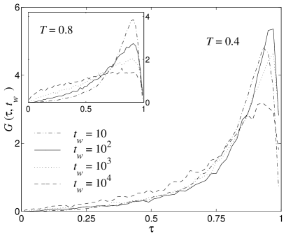
Figure 7: The location of the energy minimum within a valley entered at time $t_{w}$ in $3d$ spin glasses with $N=16^{3}$ spins. The abscissa is the time relative to the entry and exit times. The figure illustrates the highly right-skewed distribution found for all low $T$, independent of $t_{w}$. The insert shows that for higher $T$ the distribution flattens out as the age $t_{w}$ of the system grows.

In measuring the distribution of $\tau$, we keep track of the age $t_{w}$ at the time of entry, by selecting entry times for a range of different $t_{w}$. From the outset, the empirical distribution $G(\tau\mid t_{w})$ could depend on $t_{w}$, but, as shown by Fig. 7, there is practically no dependence, except for $T$ close to the critical temperature.

The right-skewed form of $G$ for lower $T$ values (the picture is the same for any $T\leq 0.6$) implies that by far the greatest part of $t_{r}$ is spent before hitting the lowest minimum: the system explores several sub-valleys, each identified by its own local minimum, while it slides towards states of lower energy. Equilibrium-like fluctuations can only occur after the state of lowest energy which remains at the bottom of the valley is hit. This time interval is small compared to the total residence time, but nevertheless grows steadily with the valley index.

Since the measured shape of $G$ at low $T$ is almost $t_{w}$ invariant, the distributions of both $t_{r}$ and $t_{hit}$ must both scale as $t_{w}^{\mu}$. We conclude that the process of hitting the lowest minimum in a valley at low $T$ is limited by internal barrier crossing events, and that these barriers themselves grow as the age increases and the valleys become larger. The landscape geometry is thus invariant under a time dilation, and hence self-similar, in agreement with the general properties of a log-Poisson process. The temperature independence of the distribution at low $T$ leads to the same conclusion: Lowering the temperature means exploring smaller valleys, which nevertheless retain the same internal structure within a range of low temperatures.

As the temperature gets closer to the critical temperature, a waiting time dependence appears: $G(\tau)$ remains peaked around $\tau\simeq 0.9$, but smaller values of $\tau$ become gradually more probable. The corresponding flattening of the distribution of $G(\tau)$ for $T=0.8$, a high temperature, is shown in the insert of Fig. 7. Since the number of potentially new valleys diminishes in time because of the lack of new low energy records, $G$ must eventually become highly left-skewed. While only a very slow trend towards this situation can be seen in the main panel, the data for the higher temperature in the insert seems to be heading in that direction, in accordance with equilibration happening much faster at high $T$ than low $T$.

We end this section by noting that, like most other quantities presented in this paper, similar results for $G(\tau\mid t_{w})$ are found across all systems simulated.

VI Coarse grained landscape description

Having argued that log-Poisson statistics is a (slightly) idealized description which leads to pure aging and other dynamical features found in experiments, we turn to the physical mechanism behind the selection of the attractors and, more broadly, consider the implications of our results for pertinent mesoscopic models of complex landscapes. We do not attempt to deal with domain growth and other real space issues in any detail. These aspects, though very important for a complete understanding of complex relaxation, are too strongly connected to quasi-equilibrium issues which lie beyond the scope of this paper.

The applicability of log-Poisson statistics to barrier records only implies that the trajectory fully decorrelates between successive events, as can be expected for an activated process in a landscape with many local minima. The new and important information about the landscape geometry lies in the fact that barrier records are required in order to find new minima records. This explains why the log-Poisson statistics is equally relevant for barriers as for minima. Secondly, and more importantly, it implies that the least stable, or marginally stable among the available attractors are those selected. Indeed, if at some stage, very deep minima were to follow a shallow barrier, subsequent barrier records would not produce new states of record-low energy, and the log-Poisson description would fail.

The close match between the depth of a valley and the magnitude of the barrier record giving access to it implies a quasi-continuum of available attractors and was first noticed in connection with the noisy dynamics of a driven dissipative system Sibani93a , where the phenomenon was dubbed noise adaptation. That complex memory behavior is linked to marginal stability of metastable attractors has long been known for noiseless models of Charge Density Waves Coppersmith87 ; Tang87 . The extremely simple automaton model of Tang et al. Tang87 describes a sheet of elastically coupled ‘balls’ driven along a sinusoidal potential by a pulsed external force. A recent study of a noisy version of this model Sibani01 shows that its non-equilibrium dynamics is described by log-Poisson statistics and that the age of the system can be reset by a change of the elastic coupling constant.

The physical origin of the bias towards shallow attractors in thermal glassy dynamics is likely to be entropic, i.e. simply the fact that shallow attractors vastly outnumber deeper ones, in line with the general observation that quenches usually produce poor minima. To support such bias for a range of low temperatures, the density of energy minima must dwarf the Boltzmann factor and hence increase at least exponentially with the energy. This concurs with the outcome of numerical exhaustive investigations of the local configuration space structure of different glassy systems Sibani93 ; Sibani98 ; Sibani94 ; Schon98 ; Schon00 ; Klotz98 ; Schon02 which were performed with the lid method Sibani93 ; Sibani99 . In all cases the local density of states and the local density of minima are nearly exponential functions of the energy.

An exponential density of states in connection with activated dynamics implies a dynamical glass transition. This exact feature was built into the tree model of complex relaxation proposed and analyzed by Grossmann et al. Grossmann85 and later studied in more detail in Hoffmann85 ; Sibani87 . It is also incorporated in the even simpler trap model of Bouchaud Bouchaud92 which, nonetheless, is very different from tree models in one important respect: trees have the lowest connectivity possible for a connected set, while each trap of the trap model is connected to all others.

Log-Poisson statistics only applies as long as new and gradually more stable valleys remain available to the dynamics. The simplest way of modeling inequivalent valleys is through a hierarchy of energy barriers separating degenerate states, which are organized in either a linear array Joh96 or in a tree graph. Beside the models already mentioned, the latter approach is followed in Sibani87 ; Joh96 ; Schreckenberg85 ; Sibani86 ; Sibani89 ; Hoffmann90 . Many important features of complex relaxation can be reproduced in this model, but not the fact that in many systems, including spin glasses, the energy decreases logarithmically with the age. This can be achieved by introducing non-degenerate local minima, as done in the so-called LS tree Hoffmann97 ; Sibani91 . The minima have energies which on average decrease linearly with the size of the barrier overcome, i.e. in the same overall fashion as Fig. 4.

In Bouchauds model, trap energies are exponentially distributed and hence non-degenerate. That deeper minima are gradually explored is a statistical consequence of the (assumed) infinite average of the residence time in a trap. If traps and valleys can be identified, the results of Section V.3 are at variance with this interpretation. The average residence time, which equals $t_{w}$ for $\alpha=2$, is, in practice, slightly lower than $t_{w}$. This is again reminiscent of the situation encountered in tree models Hoffmann97 ; Sibani87 ; Schreckenberg85 ; Sibani86 ; Sibani89 ; Hoffmann90 ; Sibani91 . The distribution of barriers in tree models has a lower cut-off, unlike the fractal description of configuration space of Dotsenko Dotsenko85 ; Vincent91 , which better captures the growing importance of gradually smaller barriers as the temperature decreases.

A last important issue is the connection between the energy barrier separating two configurations and the distance between them. For spin glasses the relevant metric is the Hamming distance, which, according to Figs. 3 and 4, on average bears a linear relationship to the energy barrier. A similar result was found in numerical work on the SK model Sherrington75 by Nemoto88 ; Vertechi89 , and by the lid-method (i.e. exact exhaustive enumeration) in Sibani94 for short range spin glasses. Since the latter investigations deal with the small scale structures inside a ‘pocket’, while the present ones are concerned with the large scale structures explored by the non-equilibrium dynamics, the agreement in their outcome is further evidence of a self-similar landscape structure. Interestingly, the largest distance which can be achieved for a fixed energy barrier grows exponentially with the barrier Sibani98 . A linear relationship between energy and Hamming distance is assumed in tree models of aging dynamics, see e.g. Sibani89 , and also in the barrier model Joh96 . This is, however, not a crucial assumption for aging, and other types of functional relationships can also be utilized Hoffmann97 successfully.

VII Summary and outlook

In this paper we have presented a general ‘non-invasive’ statistical method for complex energy landscape exploration, especially designed to provide information on the metastable states actually explored by an unperturbed aging process following a quench. The method has been thoroughly tested on Ising spin glasses, and the results obtained both match and extend the established knowledge about spin glasses. In particular, most quantities investigated obey simple scaling laws with universal scaling exponents. The view which emerges is that non-equilibrium aging dynamics is steered by energy barrier records, which are the only events capable of opening the route to new valleys. Since this description has previously been shown to apply to driven dissipative models and to evolution modeling, a possible unified theory for non-equilibrium glassy dynamics seems within reach.

A more complete picture can be obtained by looking more closely into the fluctuation dynamics which may differ across different systems. For spin glasses we have argued that real space domains of (pseudo) thermalized spins relax independently as long as the system as a whole remains in the same valley. The present method opens the possibility of identifying the quasi-equilibrium clusters as defined by the dynamics itself: These clusters are separated by a backbone of spins whose orientation remains fixed within each valley and changes slowly from one valley to the next, as seen in Fig. 3. After the lowest energy state in the valley has been hit and before the next valley is entered, there is no drift towards the global minimum. Hence, the spins fall into two categories only: those which are frozen, and those which fluctuate in a quasi-equilibrium fashion. The quasi-equilibrium clusters can thus be extracted and their statistical properties, such as e.g. the density of states, can be studied for each cluster separately.

Acknowledgments: This project has been supported by Statens Naturvidenskabelige Forskningsråd through a block grant and by the Danish Center for Super Computing with computer time on the Horseshoe Linux Cluster. We are grateful to J. Christian Schön for many discussions, and, in particular, for pointing out a flawed mathematical argument in an early version of this work.

References

- [1] W. Reim, R. H. Koch, A. P. Malozemoff, M. B. Ketchen, and H. Maletta, Phys. Rev. Lett. 57, 905 (1986).
- [2] P. Refrigier and M. Ocio, Revue Phys. Appl. 22, 367 (1987).
- [3] J.-O. Andersson, J. Mattsson, and P. Svedlindh, Phys. Rev. B 46, 8297 (1992).
- [4] P. Granberg, L. Sandlund, P. Nordblad, P. Svedlindh, and L. Lundgren, Phys. Rev. B 38, 7097 (1988).
- [5] P. Granberg, L. Lundgren, and P. Nordblad, J. Magn. and Magnetic Materials 90, 228 (1990).
- [6] C. Schultze, K. H. Hoffmann, and P. Sibani, Europhys. Lett. 15, 361 (1991).
- [7] K. Hoffmann, S. Schubert, and P. Sibani, Europhys. Lett. 38, 613 (1997).
- [8] A. V. Kityk, M. C. Rheinstädter, K. Knorr, and H. Rieger, Phys. Rev. B 65, 14415 (2002).
- [9] M. Nicodemi and H. J. Jensen, J. Phys A 34, 8425 (2001).
- [10] P. Sibani and C. M. Andersen, Phys. Rev. E 64, 021103 (2001).
- [11] L. Bureau, T. Baumberger, and C. Caroli, cond-mat/0202245 (2002).
- [12] A. Hannemann, J. C. Schön, M. Jansen, and P. Sibani, cond-mat/0212245 (2002).
- [13] P. Sibani and J. Dall, cond-mat/0206535 (2002).
- [14] P. Sibani and P. B. Littlewood, Phys. Rev. Lett. 71, 1482 (1993).
- [15] P. Sibani and J. Dall, to appear in Europhys. Lett. .
- [16] S. Coppersmith and P. Littlewood, Phys. Rev. B 36, 311 (1987).
- [17] K. Jonason, E. Vincent, J. Hamman, J. P. Bouchaud, and P. Nordblad, Phys. Rev. Lett. 81, 3243 (1998).
- [18] F. H. Stillinger and T. A. Weber, Phys. Rev. A 28, 2408 (1983).
- [19] K. Nemoto, J. Phys. A 21, L287 (1988).
- [20] O. M. Becker and M. Karplus, J. Chem. Phys. 106, 1495 (1997).
- [21] A. Crisanti and F. Ritort, J. Phys. Cond. Matt. 14, 1381 (2002).
- [22] S. Mossa, G. Ruocco, F. Sciortino, and P. Tartaglia, Phil. Mag. B 82, 695 (2002).
- [23] P. Sibani, C. Schön, P. Salamon, and J.-O. Andersson, Europhys. Lett. 22, 479 (1993).
- [24] P. Sibani, Physica A 258, 249 (1998).
- [25] J. C. Schön, H. Putz, and M. Jansen, J. Phys. Cond. Matt. 8, 143 (1996).
- [26] J.-O. Andersson and P. Sibani, Physica A 229, 259 (1996).
- [27] M. Palassini and A. P. Young, Phys. Rev. Lett. 83, 5126 (1999).
- [28] J. Houdayer and O. C. Martin, Europhys. Lett. 49, 794 (2000).
- [29] J. Lamarcq, J. P. Bouchaud, O. C. Martin, and M. Mezard, Europhys. Lett. 58, 321 (2002).
- [30] M. A. C. Wevers, J. C. Schön, and M. Jansen, J. Phys. Cond. Matt. 11, 6487 (1999).
- [31] P. Sibani, M. Schmidt, and P. Alstrøm, Phys. Rev. Lett. 75, 2055 (1995).
- [32] P. Sibani, M. Brandt, and P. Alstrøm, Int. J. Modern Phys. B 12, 361 (1998).
- [33] P. Sibani and A. Pedersen, Europhys. Lett. 48, 346 (1999).
- [34] S. A. Kauffman and S. Levine, J. Theor. Biol. 128, 11 (1987).
- [35] M. Hall, K. Christensen, S. A. di Collabiano, and H. J. Jensen, Phys. Rev. E 66, 011904 (2002).
- [36] B. Rinn, P. Maass, and J.-P. Bouchaud, Phys. Rev. Lett. 84, 5403 (2000).
- [37] G. F. Rodriguez, G. G. Kenning, and R. Orbach, Phys. Rev. Lett. 91, 037203 (2003).
- [38] J. Dall and P. Sibani, in preparation .
- [39] J. Dall and P. Sibani, Comp. Phys. Comm. 141, 260 (2001).
- [40] J. Kisker, L. Santen, M. Schreckenberg, and H. Rieger, Phys. Rev. B 53, 6418 (1996).
- [41] P. Sibani and P. Schriver, Phys. Rev. B 49, 6667 (1994).
- [42] P. Sibani, R. van der Pas, and J. C. Schön, Comp. Phys. Comm. 116, 17 (1999).
- [43] J. C. Schön and P. Sibani, J. Phys. A 31, 8165 (1998).
- [44] J. C. Schön and P. Sibani, Europhys. Lett. 49, 196 (2000).
- [45] M. R. Leadbetter, G. Lindgren, and H. Rotzen, Extremes and related properties of random sequences and processes (Springer, New York, 1983).
- [46] G. S. Grest, C. M. Soukoulis, and K. Levin, Phys. Rev. Lett. 56, 1148 (1986).
- [47] J. Bouchaud, J. Phys. I France 2, 1705 (1992).
- [48] E. Vincent, J. P. Bouchaud, D. S. Dean, and J. Hammann, Phys. Rev. B 52, 1050 (1995).
- [49] L. Berthier and J.-P. Bouchaud, Phys. Rev. B 66, 054404 (2002).
- [50] E. Vincent, J. Hammann, M. Ocio, J.-P. Bouchaud, and L. F. Cugliandolo, in Lecture notes in physics: Complex Behaviour of Glassy Systems, edited by M. Rubí and C. Pérez-Vicente (Springer, 1997), vol. 492, pp. 184–219.
- [51] J.-P. Bouchaud, in Soft and Fragile Matter, edited by M. E. Cates and M. R. Evans (1999), pp. 285–304.
- [52] C. Tang, K. Wiesenfeld, P. Bak, S. Coppersmith, and P. Littlewood, Phys. Rev. Lett. 58, 1161 (1987).
- [53] T. Klotz, S. Schubert, and K. H. Hoffmann, J. Phys. Cond. Matt. 10, 6127 (1998).
- [54] J. Schön, J. Phys. Chem. A 106, 10886 (2002).
- [55] S. Grossmann, F. Wegner, and K. H. Hoffmann, J. Physique Letters 46, 575 (1985).
- [56] K. Hoffmann, S. Grossmann, and F. Wegner, Z. Phys. B 60, 401 (1985).
- [57] P. Sibani, Phys. Rev. B 35, 8572 (1987).
- [58] Y. G. Joh, R. Orbach, and J. Hamman, Phys. Rev. Lett. 77, 4648 (1995).
- [59] M. Schreckenberg, Z. Phys. B 60, 483 (1985).
- [60] P. Sibani, Phys. Rev. B 34, 3555 (1986).
- [61] P. Sibani and K. H. Hoffmann, Phys. Rev. Lett. 63, 2853 (1989).
- [62] K. Hoffmann and P. Sibani, Z. Phys. B 80, 429 (1990).
- [63] P. Sibani and K. Hoffmann, Europhys. Lett. 16, 423 (1991).
- [64] V. S. Dotsenko, J. Phys. C 18, 6023 (1985).
- [65] E. Vincent, in Recent progress in random magnets, edited by D. H. Ryan (Mc Gill University, 1991), pp. 209–246.
- [66] D. Sherrington and S. Kirkpatrick, Phys. Rev. Lett. 35, 1792 (1975).
- [67] D. Vertechi and M. Virasoro, J. Phys. France 50, 2325 (1989).