A NEW APPROACH TO DYNAMIC FINITE-SIZE SCALING

MEHMET DİLAVER , SEMRA GÜNDÜÇ, MERAL AYDIN^† and YİĞİT GÜNDÜÇ

Hacettepe University, Physics Department,

06532 Beytepe, Ankara, Turkey

$\dagger$ Çankaya University, Mathematics and Computer Science Department,

06530 Balgat, Ankara, Turkey

Abstract

In this work we have considered the Taylor series expansion of the dynamic scaling relation of the magnetization with respect to small initial magnetization values in order to study the dynamic scaling behaviour of $2$- and $3$-dimensional Ising models. We have used the literature values of the critical exponents and of the new dynamic exponent $x_{0}$ to observe the dynamic finite-size scaling behaviour of the time evolution of the magnetization during early stages of the Monte Carlo simulation. For $3$-dimensional Ising Model we have also presented that this method opens the possibility of calculating $z$ and $x_{0}$ separately. Our results show good agreement with the literature values. Measurements done on lattices with different sizes seem to give very good scaling.

Keywords: Ising Model, Dynamic Scaling, Time Evolution of the Magnetization

1 Introduction

The determination of the critical temperature and the corresponding critical exponents for the systems exhibiting second-order phase transitions is the major task in many areas of physics. In order to determine the critical parameters of the system there exist two approaches. Traditionally, one uses universality and the scaling relations in the equilibrium stages of the statistical mechanical system. In other words, one studies the long-time regime of the system. The second approach is to study dynamic scaling which seems to exist in the early stages of the quenching process in the system exhibiting second-order phase transition. Jansen, Schaub and Schmittmann [1] have shown that for a dynamic relaxation process, in which a system is evolving according to a dynamics of Model A [2] and is quenched from a very high temperature to the critical temperature, a universal dynamic scaling behaviour within the short-time regime exists [3, 4].

 

Monte Carlo simulations are the most commonly used tools to study statistical mechanical systems in thermal equilibrium around the phase transition point. Creating statistically independent configurations is controlled by the autocorrelations in the system which depend on the system as well as the simulation algorithm. Around the phase transition point, the correlation length grows exponentially and this results in the effect known as the critical slowing down. On finite lattices the autocorrelation time diverges as $\tau\sim L^{z}$, where $L$ is the linear size of the lattice and $z$ is the dynamic critical exponent.

 

Dynamic finite-size scaling relation is a generalized form of the finite-size scaling relation valid for the equilibrium stages. For the $k^{th}$ moment of the magnetization of a system with spatial size $L$ this relation can be written as [1]

$$M^{(k)}(t,\epsilon,{m_{0},L})=L^{(-k{\beta}/{\nu})}{\cal{M}}^{(k)}(tL^{-z},{\epsilon}L^{1/{\nu}},{m_{0}}L^{x_{0}})$$ (1)

where $\beta$ and $\nu$ are the well-known critical exponents, $t$ is the simulation time and ${\epsilon}=(T-{T_{c}})/{T_{c}}$ is the reduced temperature. In the study of the short-time dynamic scaling of a system, in addition to the critical exponents, the dynamic critical exponent $z$ and a new and independent exponent $x_{0}$ appear, where $x_{0}$ is the anomalous dimension of the initial magnetization $m_{0}$.

 

Eq.(1) can be reformulated for the time evolution of the magnetization at early stages of the simulation. For very small initial magnetization, time evolution of the magnetization undergoes a critical initial increase [1, 3] in the form

$$M(t)\sim{m_{0}}{t^{\theta}}$$ (2)

where the exponent $\theta$ is related to the exponent $x_{0}$ by $\theta=({x_{0}}-{\beta}/{\nu})/z$. The power-law behaviour relation (Eq.(2)) of the dynamic finite-size scaling is used to estimate the critical exponents $z$, $\theta$ and ${\beta}/{\nu}$. In literature, it has been shown that the dynamic behaviour of various spin models obeys the dynamic scaling relations (Eqs. (1) and (2))  [5, 6, 7, 8, 9, 10, 11, 12]; the universality of $x_{0}$ has also been studied and numerical evidence for the existence of the universality of the dynamic scaling has been given [7, 13].

 

In this work we aim to reconsider dynamic finite-size scaling by approaching the problem from a different point of view. Instead of the critical initial increase (Eq. (2)) of the magnetization used in the literature, we have used the dynamic scaling relation (Eq.(1)) by considering the Taylor series expansion of ${{M}}^{(k)}(t,{\epsilon},m_{0},L)$ with respect to small initial magnetization $m_{0}$. We have seen that the new exponent ($x_{0}$) exists not only in the initial stages, but also until the effects of the initial magnetization of the system diminish. This approach seems to give the critical exponents and the dynamic exponents with very high accuracy. In order to discuss the proposed method we have considered $2$- and $3$-dimensional Ising models which are well-studied by finite-size scaling techniques for both equilibrium and non-equilibruium stages.

 

In the next section we present the model, the method and the scaling relation for the magnetization. In section 3 numerical results for $2$- and $3$-dimensional Ising models will be reported. The last section contains the conclusions.

2 Model and the Method

In this work we have employed $2$- and $3$-dimensional Ising models which are described by the Hamiltonian

$${-\beta}H=K{\sum_{<ij>}}{S_{i}}{S_{j}}\;.$$ (3)

Here $\beta=1/kT$ and $K=J/kT$, where $k$ is the Boltzmann constant, $T$ is the temperature and $J$ is the magnetic interaction between the spins. In the Ising Model the spin variables take the values ${S_{i}}={\pm 1}$. In this work we have performed Monte Carlo simulations by using Metropolis algorithm.

 

The measurements of the thermodynamic quantities which are obtained using thermalized configurations in Monte Carlo simulations are independent of the initial configuration. Here, before the thermalization, the convergence path (to the thermalization) may be different depending on which initial configuration is used. Although the system reaches the same thermalized configurations in the long-time regime, the convergence path is highly sensitive to the initial configuration. In this work we propose to consider the dynamics of the thermalization for a system with two different initial configurations, in order to obtain the new dynamic index $x_{0}$. One initial configuration can be considered as the configuration with vanishing initial magnetization. The second initial configuration can be taken with arbitrary, but small initial magnetization. The dynamic finite-size scaling form of the $k^{th}$ moment of the magnetization is given by Eq.(1). At the critical point $({\epsilon}=0)$, for small initial magnetization ($m_{0}$) values, the function given in Eq.(1) can be expanded into Taylor series around $m_{0}=0$ resulting in

$$M^{(k)}(t,0,{m_{0}},L) = L^{-k{\beta}/{\nu}}{\cal{M}}^{(k)}(tL^{-z},0,0)+$$

$$\frac{\partial{\cal{M}}^{(k)}(tL^{-z},0,{m_{0}})}{\partial{m_{0}}}{\mid}_{{m_{0}}=0}{m_{0}}L^{{x_{0}}-{k\beta}/{\nu}}+O({m_{0}}^{2})\;.$$

The first term in this expansion has no $m_{0}$ dependence and it can be calculated through Monte Carlo simulations by considering the initial configuration with vanishing initial magnetization. The $m_{0}$-dependent terms (second and higher order terms in the expansion) can be represented by a function $M_{s}(t,0,m_{0},L)$ which is basically

$$M_{s}(t,0,m_{0},L)\,=\,\frac{\partial{\cal{M}}^{(k)}(tL^{-z},0,{m_{0}})}{\partial{m_{0}}}{\mid}_{{m_{0}}=0}{m_{0}}L^{{x_{0}}-{k\beta}/{\nu}}+O({m_{0}}^{2})\;$$ (5)

and it can be obtained by calculating the difference of $M^{(k)}(t,0,m_{0},L)$ and $M^{(k)}(t,0,0,L)$. This means it has the form,

$$M_{s}(t,0,m_{0},L)=M^{(k)}(t,0,m_{0},L)-M^{(k)}(t,0,0,L).$$ (6)

Here $M^{(k)}(t,0,0,L)$ corresponds to the first term in the expansion. The terms $M^{(k)}(t,0,m_{0},L)$ and $M^{(k)}(t,0,0,L)$ can be measured through Monte Carlo simulations using two different initial configurations, one with initial magnetization $m_{0}$ and the other one with vanishing initial magnetization.

 

The function given in Eqs.(5) and (6) contains all $m_{0}$ dependence. The thermalized configurations are independent of the initial magnetization, hence $M_{s}(t,0,m_{0},L)$ is a decaying function. This function is expected to be a function of the autocorrelation time and the initial magnetization. In this work, we have chosen an exponentially decaying function in the form

$$M_{s}(t,0,m_{0},L)=f(m_{0},L)\;e^{{-(t/\tau(L))}^{\phi(L)}}.$$ (7)

Here $t$ is the simulation time, $\tau(L)$ is the autocorrelation time and $\phi(L)$ is an exponent which is related to the initial slip. If this form fits the data, two dynamical exponents can be calculated separately. $f(m_{0},L)$ is a $m_{0}$-dependent function, but it is has no autocorrelation time dependence. Hence the new dynamic scaling exponent $x_{0}$ can be calculated from the size dependence of this function for small values of $m_{0}$. The autocorrelation time and hence $z$ can be calculated from the decay rate of $M_{s}(t,0,m_{0},L)$. The validity of our assumptions has been tested by fitting the function given in Eq(7) to our data and the results are presented in Section 3.

 

For very small initial magnetization values, it is expected that the leading term in the expansion (Eq. (2)) is dominant and the rest of the terms (represented by the function $M_{s}(t,0,m_{0},L)$) is in the same order of magnitude with the simulation errors. Increasing initial magnetization results in a sizeable $m_{0}$-dependent term in Eq. (2). In this range of $m_{0}$ one can expect that $M_{s}(t,0,m_{0},L)$ scales like $L^{x_{0}-\beta/\nu}$. Further increase in $m_{0}$ reduces the reliability of such scaling since the contribution of higher order terms in the expansion (Eq. (2)) becomes effective. In our simulations we have used different $m_{0}$ values to investigate the proposed scaling behaviour of $M_{s}(t,0,m_{0},L)$. To test the scaling we have used the literature values of $\beta/{\nu}$ and $x_{0}$ for $2$- and $3$-dimensional Ising models and also calculated the dynamic exponents $z$ and $x_{0}$ for $3$-dimensional model through a fit to our Monte Carlo data.

3 Results and Discussions

We have studied $2$-and $3$-dimensional Ising models evolving in time according to the dynamics of the Model A[2]. We have prepared the lattices with varying initial magnetization values starting from $m_{0}=0$. Totally random initial configurations are quenched at the corresponding infinite lattice critical temperature. Simulations are performed by using Metropolis algorithm on lattices with linear sizes $L=512,640,768,896$ and $L=32,64,96$ for $2$- and $3$-dimensional Ising models respectively. For error calculations we have binned data points obtained from $4000$ to $15000$ independent runs for $3$-dimensional model, and $50000$ to $500000$ independent runs for $2$-dimensional model, starting from randomly prepared configurations. For $3$-dimensional model, $3000$ iterations are performed for each independent run. For $2$-dimensional model there are two different sets of runs. One set of data is obtained after $500$ iterations for each independent run and for the other set of data, each independent run includes $10000$ iterations.

 

The dynamic critical exponent $z$ has a little dependence on dimension for local algorithms. For a given numbers of spins, the saturation in magnetization can be observed after relatively small number of iterations in $3$-dimensional lattice compared two $2$-dimensional one, since the saturation is observed when the correlation length reaches the linear size of the lattice. In order to observe the behaviour of the $m_{0}$-dependent terms, one needs to study the time development of the system until both $M^{(k)}(t,0,m_{0},L)$ and $M^{(k)}(t,0,0,L)$ reach approximately the same value. In our simulation studies, we have observed that for $3$-dimensional lattice, configurations with both vanishing and non-vanishing initial magnetization reach the same value in (approximately) $3000$ iterations for the largest lattice $(L=96)$. For $2$-dimensional model, since much larger linear sizes are used, the initial configuration dependence remains after $30000$ iterations and observing the decaying behaviour of $M_{s}(t,0,m_{0},L)$ becomes extremely expensive. For this reason, we have tested our ideas for $3$-dimensional model. In $2$-dimensional lattice, we have performed simulations up to $10000$ iterations, but even this many iterations is extremely short to observe the decaying behaviour of $M_{s}(t,0,m_{0},L)$. Nevertheless, it is sufficient to test the scaling behaviour and to obtain the new dynamic critical exponent $x_{0}$.

 

In Figure 1, the magnetization data are presented for vanishing initial magnetization and for $m_{0}\approx 0.1$ in $3$-dimensional Ising Model with linear sizes $L=32,64,96$. The magnetization data converge approximately to the same value for both initial configurations after approximately $500(L=32),1500(L=64),3000(L=96)$ iterations. The differences between the data obtained by starting from different initial magnetizations are large initially for large lattices and vanishes after above mentioned number of iterations are reached. The final magnetization value decreases as the lattice size increases, and the magnetization is smaller initially for vanishing $m_{0}$. The function $M_{s}(t,0,m_{0},L)$ which represents the difference between $M^{(k)}(t,0,m_{0},L)$ and $M^{(k)}(t,0,0,L)$ is given in Figure 2, for $m_{0}\approx 0.1$ and for linear sizes, $L=32,64,96$ in $3$-dimensional lattice. The function $M_{s}(t,0,m_{0},L)$ is a decreasing function with an initial value proportional to the lattice size $L$. Despite the fact that our main aim is not to obtain the dynamical critical exponent $(z)$, since we are interested in the functional form of the $m_{0}$-dependent term and the speed of its decay, we have fitted our data to the functional form $(\tau\sim L^{z})$ and obtained $z$ from the fit results. We have fitted the data to the exponential function given in Eq.(7). This function fits the data reasonably well, as it can be seen from Figure 2. The correlation times $(\tau)$ obtained from the fit are $\tau(L)=80,\;372,\;839$ for $L=32,64,96$ respectively. The errors are in the order of one. We have fitted the functional form $(\tau\sim L^{z})$ to our data and we have obtained the value for $z$ as $z=2.04\pm 0.07$ for $3$-dimensional model. Figure 3 shows the fitted function and the data points for three lattice sizes used.

 

As it is mentioned in Section 2, the function $M_{s}(t,0,m_{0},L)$ representing $m_{0}$-dependent terms scales like $L^{z\theta}$. Here we have used the literature values of the exponent $\theta=(x_{0}-\beta/\nu)/z$, $\theta=0.191(2)$ [13] and $\theta=0.108(2)$ [11] for $2$- and $3$-dimensional Ising models respectively, to test the scaling. The exponent $z\,\theta=x_{0}-\beta/\nu$ is obtained from these literature values of both $\theta$ and $z$. For $2$-dimensional Ising Model, the value of the dynamic critical exponent $z$ for Metropolis algorithm varies from $2.13$ to $2.18$  [3, 4, 5, 18, 19, 20, 21, 22, 23, 24]. For the $3$-dimensional case, the equilibrium case, the value of the dynamic critical exponent is $z=2.04(3)$ [25], while from the dynamic scaling, $z$ ranges from $2.032(11)$ to $2.052(17)$ [11]. We have used $z=2.18$ and $z=2.04$ for $2$- and $3$-dimensional Ising models respectively. The scaling of the function $M_{s}(t,0,m_{0},L)$ obtained from the Monte Carlo data for $3$-dimensional model is given in Figure 4. As it can be seen from this figure, these terms are scaled reasonably well. We have also fitted the data to a function to obtain the best fit and to obtain the value for $z\theta$. Our value $z\,\theta=0.27{\pm}0.03$ (for $3$-dimensional model) is slightly larger than the value in the literature.

 

For $2$-dimensional Ising Model, the autocorrelation time $(\tau)$ is extremely long for the lattice sizes we use. Consequently, we didn’t aim to see the decaying form of $M_{s}(t,0,m_{0},L)$. Instead we have tested the scaling behaviour of $M_{s}(t,0,m_{0},L)$. In Figure 5, we have presented the data for $M_{s}(t,0,m_{0},L)$ for after $500$ iterations and Figure 6 shows the scaling of the data when the literature values are used.

4 Conclusions

The short-time dynamic behaviour of the magnetization is studied in $2$- and $3$-dimensional Ising models. The time-dependent magnetization profiles with different initial magnetization ($m_{0}$) values exhibit an initial increase during the time scale set by the initial magnetization, the dynamic critical exponent ($z$) and the new dynamic exponent ($x_{0}$). After a long-time ($t\sim L^{z}$), all profiles gradually join together, since in the long-time regime the effects of the initial conditions are ignorable. In this work we aimed to study the effects of the initial configurations on magnetization by using Monte Carlo simulation. This can be observed by expanding the magnetization around $m_{0}=0$. This expansion (Eq. (1)) gives a leading term which is independent of $m_{0}$ and the terms containing the information of how the initial configuration is prepared.

 

In this approach, the dynamic critical behaviour can be studied by using the data from the early stages of the Monte Carlo simulation. In order to obtain a relation between the size and the initial magnetization dependence of the Monte Carlo data, we have considered both vanishing and non-vanishing initial magnetization runs. The iteration by iteration differences of these two sets of runs yield the initial magnetization dependence of the system. Using different lattice sizes we have shown that the proposed scaling holds. We have also shown that the dynamic finite-size scaling is valid not only for the very early stages (within $100$ iterations) of the Monte Carlo runs, but it is valid until the effects of the the initial magnetization diminish.

 

In order to test our proposed approach, we have employed the literature values of $\beta/\nu$, $z$, $x_{0}$ and we have observed a good scaling behaviour for $m_{0}$-dependent terms for the lattice sizes we used. Such a good scaling gives hopes for the applicability of this approach to a wide range of statistical mechanical systems for calculations of both dynamic and equilibrium critical exponents.

Figure Captions

Figure 1. Magnetization data for $3$-dimensional Ising Model with linear lattice sizes $L=32,64,96$, with vanishing and nonzero initial magnetization ($m_{0}\approx 0.1$) for each size, as a function of simulation time $t$. The curves for vanishing initial magnetization start from the origin.

 

Figure 2. The function $M_{s}(t,0,m_{0},L)$ corresponding to $m_{0}$-dependent terms in the expansion as a function of simulation time $t$, for $3$-dimensional Ising Model. The plot of the function fitted to the form given in Eq.(7) is also shown.

 

Figure 3. The autocorrelation time $\tau(L)$ as a function of the linear lattice size $L=32,64,96$ in $3$-dimensional Ising Model. The function fitted to the form $\tau\sim L^{z}$ is also shown.

 

Figure 4. Scaled form of $M_{s}(t,0,m_{0},L)$ obtained from the simulation data (given in Figure 2), for $3$-dimensional Ising Model.

 

Figure 5. $M_{s}(t,0,m_{0},L)$ obtained from the simulation data as a function of simulation time $t$ for $2$-dimensional Ising Model ($m_{0}\approx 0.07$).

 

Figure 6. Scaled form of the data given in Figure 5 for function $M_{s}(t,0,m_{0},L)$ for $2$-dimensional Ising Model.

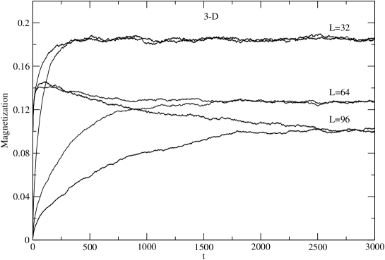
Figure 1:

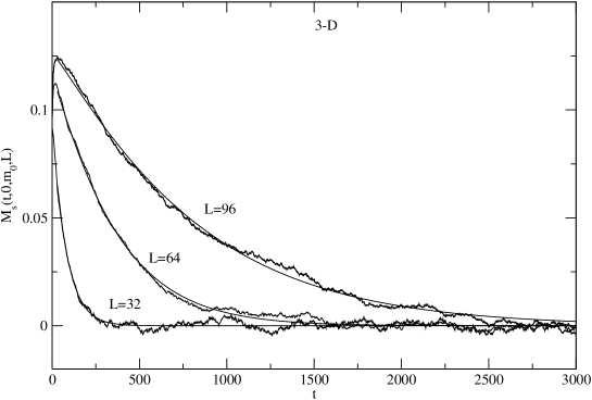
Figure 2:

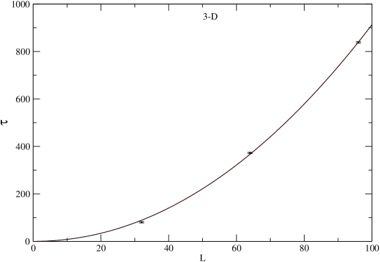
Figure 3:

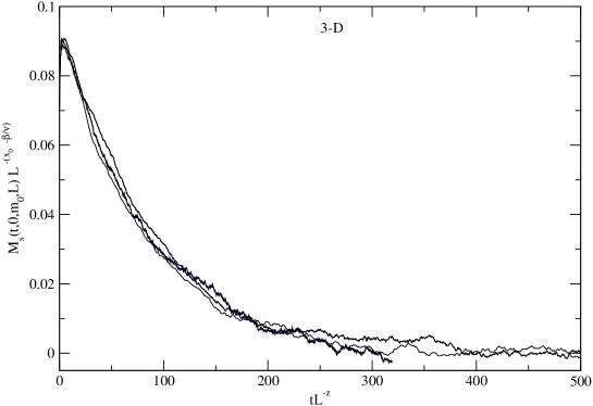
Figure 4:

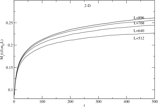
Figure 5:

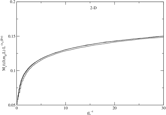
Figure 6:

References

- [1] H. K. Janssen, B. Schaub and B. Schmittmann, Z. Phys. B73, 539 (1989).
- [2] P. C. Hohenberg and B. I. Halperin, Rev. Mod. Phys. 49, 435 (1977).
- [3] B. Zheng, Int. J. Mod. Phys. B12, 1419 (1998).
- [4] B. Zheng, Physica A 283, 80 (2000).
- [5] N. Ito, Physica A 192, 604 (1993).
- [6] L. Schülke and B. Zheng, Phys. Lett. A204, 295 (1995).
- [7] K. Okano, L. Schülke, K. Yamagishi and B. Zheng, Nucl. Phys. B485 [FS], 727 (1997).
- [8] H. P. Ying, B. Zheng, Y. Yu and S. Trimper, Phys. Rev. E63, R35101 (2001).
- [9] H. J. Luo, L. Schülke and B. Zheng, Mod. Phys. Lett. B13, 417 (1999).
- [10] B. Zheng, M. Schulz and S. Trimper, Phys. Rev. E59, R1351 (1999).
- [11] A. Jaster, J. Mainville, L. Schülke and B. Zheng, J. Phys. A: Math. Gen. 32, 1395 (1999).
- [12] K. Okano, L. Schülke and B. Zheng, Phys.Rev. D57, 1411 (1998).
- [13] J. B. Zhang, L. Wang, D. W. Gu, H. P. Ying and D. R. Ji, Phys. Lett. A262, 226 (1999).
- [14] H. W. J. Blöte, E. Luitjen, J. R. Heringa, J. Phys. A: Math. Gen. 28, 6289 (1995).
- [15] A. J. Liu and M. E. Fisher, Physica A156, 35 (1989).
- [16] H. W. J. Blöte, A. Compagner, J. H. Croockewit, Y. T. J. C. Fonk, J. R. Heringa, A. Hoogland, T. S. Smit and A. L. van Willigen, Physica A161, 1(1989).
- [17] G. S. Pawley, R. H. Swendsen, D. Y. Wallace and K. G. Wilson, Phys. Rev. B29, 4030 (1984).
- [18] S. Tang and D. P. Landau, Phys. Rev. B36, 567 (1987).
- [19] D. P. Landau, S. Tang and S. Wansleben, Journal de Physique Colloque 49, C8 (1988).
- [20] Z. B. Li, L. Schülke and B. Zheng, Phys. Rev. Lett. 74, 3396 (1995).
- [21] Z. B. Li, L. Schülke and B. Zheng, Phys. Rev. E53, 2940 (1996).
- [22] P. Grassberger, Physica A214, 547 (1995).
- [23] M. P. Nightingale and H. W. J. Blöte, Phys. Rev. Lett. 76, 4548 (1996).
- [24] U. Gropengiesser, Physica A215. 308 (1995)
- [25] S. Wansleben and D. P. Landau, Phys. Rev. B43, 6006 (1991).