The wave-vector power spectrum of the local
tunneling density of states: ripples in a d-wave sea

Abstract

A weak scattering potential imposed on a $CuO_{2}$ layer of a cuprate superconductor modulates the local density of states $N(x,\omega)$. In recently reported experimental studies Hof02 ; How02 ; McE02 , scanning-tunneling maps of $N(x,\omega)$ have been Fourier transformed to obtain a wave-vector power spectrum. Here, for the case of a weak scattering potential, we discuss the structure of this power spectrum and its relationship to the quasi-particle spectrum and the structure factor of the scattering potential. Examples of quasi-particle interferences in normal metals and $s$- and $d$-wave superconductors are discussed.

I Introduction

A weak scattering potential imposed on the $CuO_{2}$ layer of a cuprate superconductor creates ripples in the local tunneling density of states $N(x,\omega)$ due to quasi-particle interference scattering. It was suggested that scanning tunneling measurements of the spatial and frequency structure of $N(x,\omega)$ could provide information on the $k$ and $\omega$ dependence of the gap BFS93 . Recently, the introduction of high-resolution Fourier-transform scanning tunneling microscopy Hof02 ; How02 ; McE02 (FT-STM) has provided a powerful new technique for studying this. In this approach, a BISCO crystal is cleaved exposing a $BiO_{2}$ layer. Then an STM measurement of the local tunneling conductance $dI(V,x)/dV$ is taken over a predetermined $L\times L$ grid of points that cover a region of order 600Å$\times$600Å. Assuming that the tunneling conductance is proportional to the underlying density of states of the $Cu\,O_{2}$ layer MB01 , these measurements give an STM map of the local tunneling density of states $N(x,\omega)$ with $\omega=eV$. This map is then Fourier transformed,

$$N(q,\omega)=\sum_{x_{l}\in(L\times L)}e^{-iq\cdot x_{l}}N(x_{l},\omega)~{},$$ (1)

and the wave-vector power spectrum,

$$P(q,\omega)=\frac{|N(q,\omega)|^{2}}{L^{2}}~{},$$ (2)

determined. Typically, the square root of the power spectrum, which is proportional to the magnitude of $N(q,\omega)$, is plotted and we will follow that practice as well. Here, we will discuss the structure of $P(q,\omega)$ and its relationship to the quasi-particle spectrum and the structure factor of the scattering potential.

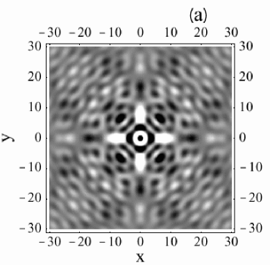
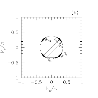
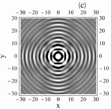
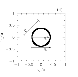
Figure 1: (a) The local tunneling density of states $N(x,\omega)$ due to scattering from a weak potential at the origin BFS93 , for (a) $\omega=0.5\Delta_{0}$ and (c) $\omega=1.1\Delta_{0}$. The length scale is set by $k_{F}^{-1}$. These results were obtained for a cylindrical Fermi surface with a $d$-wave gap $\Delta(\theta)=\Delta_{0}\cos(2\theta)$. The contours of the solid regions in (b) and (d) correspond to the points where $\omega=\sqrt{\epsilon^{2}_{k}+\Delta^{2}(\theta)}$ for $\omega=0.5\Delta_{0}$ and $1.1\Delta_{0}$, respectively. The dashed line in (b) is the Fermi surface for the non-interacting system. The ${\bf q}_{\alpha}(\omega)$ wave vectors in (b), introduced in Ref. McE02 , connect the tips of various contours and ${\bf q}^{\prime}(\omega)$ connects what would be a diagonal nesting vector for the normal state Fermi surface. The ${\bf Q}_{\alpha}(\omega)$ wave vectors shown in (d) are the relevant nesting vectors when $\omega>\Delta_{0}$.

For an isotropic $s$-wave superconductor with a circular normal state Fermi surface, the ripples in $N(x,\omega)$ produced by a weak scattering center form a circular pattern whose amplitude and wave length depend upon the bias voltage $\omega=eV$. However, if the gap has $d_{x^{2}-y^{2}}$ symmetry, the ripples emanating from a scattering center appear as a characteristic set of rays whose wave length and amplitude vary with their angular direction and the size of the bias voltage $\omega=eV$BFS93 ; FB99 . Two examples of this are shown in Fig. 1. It is the STM measurements of these modulations in $N(x,\omega)$ that provide information on the wave vector and frequency dependence of the gap. Indeed, in their FT-STM power spectrum study of BISCO, Hoffman et. al Hof02 and McElroy et. al McE02 found frequency-dependent structure in $P(q,\omega)$ which they argued were consistent with the Fermi surface dependence of $\Delta(k)$ as seen from ARPES measurements Din96 . In this work Hof02 ; McE02 , these authors suggested that the FT-STM data could be analyzed in terms of a set of frequency-dependent wave vectors ${\bf q}_{\alpha}(\omega)$ which connect the tips of the constant energy contours specified by the quasi-particle dispersion relation

$$\omega=\sqrt{\epsilon^{2}_{k}+\Delta^{2}_{k}}.$$ (3)

The contours of the solid regions shown in Figs. 1(b) and (d) are the constant quasi-particle energy contours for a cylindrical Fermi surface $\epsilon_{k}=k^{2}/2m-\mu$ with a gap $\Delta_{k}=\Delta_{0}\cos{2\theta}$ for $\omega=0.5\Delta_{0}$ and $1.1\Delta_{0}$, respectively. Also shown in Fig. 1(b) are several of the ${\bf q}_{\alpha}(\omega)$ wave vectors introduced in Ref. McE02 . The wave vector ${\bf q}^{\prime}(\omega)$ is an additional wave vector that we will discuss. The wave vectors ${\bf q}_{1}(\omega)$ and ${\bf q}_{5}(\omega)$, along with their symmetry-related counter parts (not shown), are associated with the structure of the ripples in $N(x,\omega)$ seen along the $x$ and $y$ axes of Fig. 1(a). Likewise, the wave vectors ${\bf q}_{3}(\omega)$, ${\bf q}^{\prime}(\omega)$, and ${\bf q}_{7}(\omega)$ determine the structure of the ripples along the 45^∘ axes of Fig. 1(a). In conjunction with this experimental work, Wang and Lee WL02 recently reported numerical calculations for the case of a single impurity which clearly showed the quasi-particle interference arising from ${\bf q}_{1}(\omega)$ and ${\bf q}_{7}(\omega)$. In addition, as $\omega$ is varied these calculations showed that a rich, kaleidescope-like, structure appears in the wave vector power spectrum when it is folded back into the first Brillouin zone.

In a similar way, for $\omega=1.1\Delta_{0}$, the wave vectors $Q_{\alpha}$ shown in Fig. 1(d), determine the structure of $N(x,\omega)$ seen in Fig.1 (c). Here the ripples along the $x$ and $y$-axes are associated with $Q_{2}$ and $Q_{3}$ (and their symmetry related counterparts in the $y$ direction), while those along the diagonal are associated with $Q_{1}$ (and its counterparts). In practice, when $\omega\gtrsim\Delta_{0}$, inelastic scatering leads to a damping of the ripples in $N(x,\omega)$, making the structure in $|N(x,\omega)|$ associated with the $Q_{\alpha}$ wave vectors difficult to detect.

Now, the quasi-particle interference pattern shown in Figs. 1(a) and (c) are for a single impurity. For a particular surface region over which the STM measurements are made, there will be an array of scatterers leading to a complex overlap of ripples. Here we will discuss how the Fourier transformed wave vector power spectrum $P(q,\omega)$ allows one to disentangle the quasi-particle interference effects from the static structure factors of the scatterers. In Section II we show that for the case of a weak scattering potential, $P(q,\omega)$ factors into one piece which contains information on the nesting properties of the Fermi surface times a piece which is proportional to the static structure factor of the scatterers. We also note that these measurements contain information on the one electron self-energy. Various examples are analyzed to show the type of information that is in principle contained in the FT-STM data. In Section III, the case of a layered 2D superconductor is studied with results for both $s$-wave and $d$-wave gaps discussed. Section IV contains our conclusions and Appendices A and B contain more details of the calculations.

II FT-STM Power Spectrum of a 2D Normal Metallic Layer

To begin, we first consider the case of a normal metallic 2D layer. Suppose it is exposed to a weak potential

$$V=\sum_{s}\int d^{2}x\,\delta\epsilon(x)\,\psi^{\dagger}_{s}(x)\,\psi_{s}(x).$$ (4)

with $\delta\epsilon(x)$ an energy shift at $x$. For a BISCO-like system this local energy change $\delta\epsilon(x)$ could arise from secondary effects associated with disorder away from the $CuO_{2}$ plane, the regular potential of the $BiO_{2}$ layer or possibly a weak static stripe potential. This interaction creates a ripple in the one-electron Green’s function leading to a modulation in the local tunneling density of states. For the case of a weak potential which we will focus on, a Born approximation is appropriate so that the single particle Green’s function is given by

$$G(x,x^{\prime},\omega)=G_{o}\left(x-x^{\prime},\omega\right)+\int d^{2}{x^{\prime\prime}}\,G_{o}(x-x^{\prime\prime},\omega)\,\delta\epsilon(x^{\prime\prime})\,G_{o}(x^{\prime\prime}-x^{\prime},\omega).$$ (5)

Here, $G_{o}(x,\omega)$ is the Green’s function of the unperturbed system. Then the change in the single spin tunneling density of states at position $x$ is given by

$$\delta N(x,\omega)=-\frac{1}{\pi}\ Im\int d^{2}{x^{\prime\prime}}\,G_{o}(x-x^{\prime\prime},\omega)\,\delta\epsilon\,(x^{\prime\prime})\,G_{o}(x^{\prime\prime}-x,\omega)$$ (6)

Taking the spatial Fourier transform of $\delta N(x,\omega)$, on the $L\times L$ grid of points $\{{\bf x}_{l}\}$ specified by the STM measurements, one finds for $q\neq 0$, that

$$N(q,\omega)=\sum_{x_{l}\in(L\times L)}e^{-i{q}\cdot{x_{l}}}\delta N(x_{l},\omega)=-\frac{\delta\epsilon\,(q)}{\pi}\ Im\,\Lambda\,(q,\omega)$$ (7)

with

$$\Lambda\,(q,\omega)=\int d^{2}x\,\,e^{i{q}\cdot{x}}\,G_{o}(x,\omega)\,G_{o}(-x,\omega)$$ (8)

and

$$\delta\epsilon(q)=\int\frac{d^{2}x}{a^{2}}\,\delta\epsilon(x)e^{-iq\cdot{x}}~{}.$$ (9)

Here $a$ is the lattice spacing of the $L\times L$ STM grid and $q=2\pi(n_{x},n_{y})/La$ with $n_{x}$ and $n_{y}$ integers running from $-L/2+1$ to $L/2$. The wave-vector power spectrum of the local tunneling density of states, Eq. (2), is therefore given by

$$P(q,\omega)=\frac{1}{N}\ \biggl{|}\frac{1}{\pi}Im\,\Lambda\,(q,\omega)\biggr{|}^{2}\ |\delta\epsilon(q)|^{2}.$$ (10)

Here $N=L\times L$ is the number of sites in the sampled region. Thus, in the weak scattering Born approximation, $P(q,\omega)$ separates into a piece $|Im\,\Lambda\,(q,\omega)/\pi|^{2}$ which describes the quasi-particle interference and a piece $|\delta\epsilon(q)|^{2}$ which is the static structure factor, $S(q)$, of the scattering potential.

For the random impurity case, one could imagine making STM maps over a large number of different $L\times L$ regions. Then by averaging the structure factor over these maps one would obtain

$$\frac{\langle|\delta\epsilon(q)|^{2}\rangle}{N}=n_{i}\delta\epsilon^{2}\;\;\;(q\neq 0)$$ (11)

where $n_{i}$ is the area impurity concentration and $\delta\epsilon$ is a site energy shift. In this case, $P(q,\omega)$ would simply be proportional to $n_{i}\delta\epsilon^{2}$ times the quasi-particle interference factor from a single impurity. However, this is not the way the experiments are done. Rather, a single STM map on a finite $L\times L$ grid of points covering a specific region is measured. In this case, $|\delta\epsilon(q)|^{2}$ versus $q$ exhibits fluctuations bluring the image of $|Im\Lambda(q,\omega)/\pi|$, although one can still resolve structure in false color 2D $(q_{x},q_{y})$ maps of $|N(q,\omega)|$. However, as discussed in Appendix A, by averaging the power spectrum over blocks of width $(\Delta q_{x},\Delta q_{y})$ about each $q$, the fluctuations can be reduced if the impurities are randomly distributed. Naturally, this reduces the momentum resolution. However, if the change in $q$ of the quasi-particle interference response is predominately along a given momentum direction, one can average over a region of $q$ values perpendicular to the direction of interest, reducing the fluctuations but maintaining the $q$ resolution in the direction of interest. Here we will assume that a suitable average has been done and use the impurity structure factor given by Eq. (11). Appendix A contains a further discussion of the effect of impurity induced fluctuations.

For the case in which the scattering occurs from a regular lattice such as the $Bi$ lattice, one has

$$\left|\delta\epsilon(q)\right|^{2}=\delta\epsilon^{2}N^{2}\delta_{{q},{G}_{n}}$$ (12)

Here ${\bf G}_{n}$ is a reciprocal lattice vector of the $Bi$ lattice along with the satellite wave vectors associated with the supermodulation of the $BiO_{2}$ layer. One could also have a “random” array of stripe domains with

$$\left\langle\left|\delta\epsilon(q)\right|^{2}\right\rangle\simeq N_{i}\left\{\frac{\Gamma/\pi}{(q_{x}-Q_{x})^{2}+\Gamma^{2}}+\frac{\Gamma/\pi}{(q_{y}-Q_{y})^{2}+\Gamma^{2}}+(q_{x}\rightarrow-q_{x},q_{y}\rightarrow-q_{y})\right\}\,\delta\epsilon^{2}$$ (13)

Here $Q_{x}=2\pi/l_{x}$ with $l_{x}$ the stripe spacing, $2\pi/\Gamma$ is the characteristic size of a domain and $N_{i}$ is the average number of domains in an $L\times L$ region. Here we have taken only the first $Q_{x}$ harmonic. The form factor associated with the charge distribution of the stripes suppresses the response at higher multiples of $Q_{x}$. We will examine the effect of an array of scattering centers in Section III.

Turning next to the quasi-particle interference response, we begin by looking at $G_{o}(x,\omega)$ for a free 2D electron gas. In this case, for $\omega>0$,

$$G_{o}(x,\omega)=\int\,\frac{d^{2}k}{(2\pi)^{2}}\ \frac{e^{i{k}\cdot{x}}}{\omega-\epsilon_{k}+i\delta}=-i\,\pi N(0)\,H^{(1)}_{0}\left(k(\omega)r\right),$$ (14)

with $\epsilon_{k}=k^{2}/2m-\mu$ and $mu=k_{F}^{2}/2m$. Here $N(0)=m/2\pi$ is the single spin electron density of states for the 2D free electron gas, $H^{(1)}_{0}$ is the zeroth order Hankel function of the first kind, $r=|x|$ and

$$k(\omega)=k_{F}\sqrt{1+\frac{\omega}{\mu}}.$$ (15)

When $k(\omega)r$ is large

$$G_{0}(x,\omega)\sim-i\,N(0)\ \left(\frac{2\pi}{k(\omega)r}\right)^{\frac{1}{2}}\ e^{i\left(k(\omega)r-\frac{\pi}{4}\right)}.$$ (16)

and the spatial modulation of $\delta N(x,\omega)$ which varies as the square of $G_{o}(x,\omega)$ is characterized by a wave vector

$$q\,(\omega)=2k_{F}\sqrt{1+\frac{\omega}{\mu}}.$$ (17)

The quasi-particle interference response function $\Lambda(q,\omega)$ for the 2D electron gas is calculated in Appendix B. The result of this calculation shows Kivup that

$$\frac{1}{\pi}\,Im\Lambda\,(q,\omega)=\Biggl{\{}\begin{array}[]{lr}\frac{8\pi N^{2}(0)}{q\sqrt{q^{2}-4k^{2}(\omega)}}&{\rm for}\ q>2k(\omega)\\ 0&{\rm for}\ q<2k(\omega)\end{array}$$ (18)

Thus, the wave-vector power spectrum for the 2D free electron gas has a cusp at $q$ equals $2k(\omega)$. $Im\Lambda(q,\omega)$ vanishes for $q<2k(\omega)$ and diverges as $(q-2k(\omega))^{-1/2}$ as $q$ approaches $2k(\omega)$ from larger values. As noted in the appendix, $Re\Lambda(q,\omega)$ has a similar cusp as $q$ approaches $2k(\omega)$ from below. Basically, there is just a shift of phase of $\pi/2$ in $\Lambda(q,\omega)$ when $q$ passes trough $2k(\omega)$. If the impurities are dilute, but the scattering from a given impurity is strong, one still has $P(q,\omega)$ proportional to the impurity concentration. However, in this case thnkKivelson , because of the phase of the t-matrix one will have singularities on both sides of $2k(\omega)$.

The experimental FT-STM data has been reported as the square root of the power spectrum or “the magnitude” $|N(q,\omega)|$ of the Fourier transform of the STM measurement of the local conductance map. Here we will follow this convention. For the case of weak Born scattering, the magnitude of $N(q,\omega)$ is proportional to $|Im\,\Lambda\,(q,\omega)/\pi|$. For the 2D electron gas, in Fig. 2, we have plotted $|N(q,\omega)|$ normalized to $\sqrt{n_{i}}N(0)|\delta\epsilon|/\mu$ versus $q$ for various values of $\omega/\mu$. Here, with $q$ in units of $2k_{F}$ one has

$$\left|\bar{N}(q,\omega)\right|=\frac{|N(q,\omega)|}{\sqrt{n_{i}}\ N(0)\left(\frac{|\delta\epsilon|}{\mu}\right)}=\frac{1}{2q}\ \frac{1}{\sqrt{q^{2}-\left(1+\frac{\omega}{\mu}\right)}}$$ (19)

for $(1+\omega/\mu)<q/2k_{F}$. As shown in Fig. 2, for the weak scattering case $|\bar{N}(q,\omega)|$ has a one-sided square root singularity at $q/2k_{F}=(1+\omega/\mu)^{1/2}$. This singularity is cut off and the response peak varies as $(\ell k_{F})^{1/2}$ when the quasi-particle mean-free path is taken into account. In this case

$$\left|\bar{N}(q,\omega)\right|=\frac{1}{2\pi\,q}\ \int\limits^{q^{2}-1}_{-1}d\epsilon\ \frac{\Gamma}{\left(\frac{\omega}{\mu}-\epsilon\right)^{2}+\Gamma^{2}}\ \frac{1}{\sqrt{q^{2}-(1+\epsilon)}}$$ (20)

with $\Gamma=(\ell k_{F})^{-1}$. Plots of $|\bar{N}(q,\omega)|$ versus $q$ for $\omega=0$ and several different values of $\Gamma$ are shown in Fig. 3.

Similarly, for an anisotropic system with

$$\epsilon_{k}=\frac{k^{2}_{x}}{2m_{x}}+\frac{k_{y}^{2}}{2m_{y}}-\mu$$ (21)

one finds that

$$\frac{1}{\pi}\ Im\,\Lambda\,\left(q_{x},q_{y},\omega\right)=\left\{\begin{array}[]{lccr}\frac{2}{\pi\gamma}m^{2}_{x}&\frac{1}{\sqrt{q^{2}_{x}+\gamma^{2}q^{2}_{y}}}&\frac{1}{\sqrt{q^{2}_{x}+\gamma^{2}q^{2}_{y}-8m_{x}(\omega+\mu)}}&{\rm for}\ q^{2}_{x}+\gamma^{2}q^{2}_{y}>8m_{x}(\mu+\omega)\\ 0&&&{\rm for}\ q^{2}_{x}+\gamma^{2}q^{2}_{y}<8m_{x}(\mu+\omega)\end{array}\right.$$ (22)

with $\gamma^{2}=m_{x}/m_{y}$. In this case the cusp in the power spectrum follows a locus determined by

$$q^{2}_{x}+\gamma^{2}q^{2}_{y}=8m_{x}(\mu+\omega)$$ (23)

which reflects the elliptical Fermi surface. In Fig. 4, we have plotted $|N(q,\omega)|$ for $\omega=0$ and $\gamma=3$ normalized to $\sqrt{n_{i}}(m_{x}/2\pi)|\delta\epsilon|/\mu$, which gives

$$\left|\bar{N}(q_{x},q_{y},\omega)\right|=\frac{1}{2\gamma}\ \frac{1}{\sqrt{q^{2}_{x}+\gamma^{2}q^{2}_{y}}}\ \frac{1}{\sqrt{q^{2}_{x}+\gamma^{2}q^{2}_{y}-\left(1+\frac{\omega}{\mu}\right)}}$$ (24)

with $q_{x}$ and $q_{y}$ measured in units of $2k_{F}^{x}=2(2m_{x}\mu)^{1/2}$. Here, we see that $|\bar{N}(q,0)|$ vanishes inside the ellipse Eq. (23) and has a square root divergence as $q$ approaches the ellipse. There is a reduction $\gamma=(m_{y}/m_{x})^{1/2}$ in the strength of the cusp along the $q_{y}$ direction relative to the $q_{x}$ direction that reflects the fact that the joint density of states which enters $\Lambda\,(q,\omega)$ depends on the curvature of the Fermi surface.

Turning now to the case of a tight-binding band, we consider first the simple nearest-neighbor hopping band for a square lattice with a unit lattice spacing

$$\epsilon_{k}=-2t\,\left(\cos k_{x}+\cos k_{y}\right)-\mu.$$ (25)

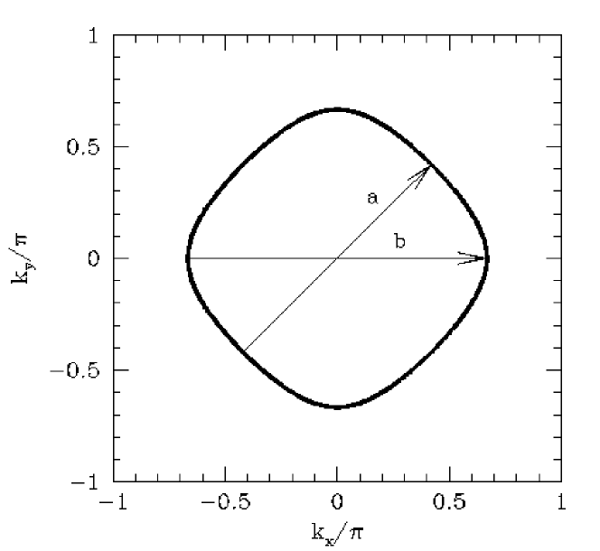
Figure 5: Fermi surface of a near-neighbor tight-binding band, Eq. (28), with $\mu/t=-1.0$ corresponding to a site filling $\langle n\rangle\approx 0.31$.

The Fermi surface is shown in Fig. 5 for $\mu=-t$, corresponding to a small filling $\langle n\rangle\approx 0.31$ which we have chosen to illustrate what happens when $Im\Lambda(q,w)$ is folded back into the first Brillouin zone. In the following tight-binding bandstructure calculations, we will assume that $N(x,\omega)$ is measured on a grid of points corresponding to the sites of the lattice. In this case,

$$\Lambda(q,\omega)=\frac{1}{N}\,\sum_{k}\,G_{0}(k+q,\omega)\,G_{0}(k,\omega)$$ (26)

with

$$G_{0}(k)=\frac{1}{\omega-\epsilon_{k}+i\delta\,sgn(\omega)}$$ (27)

Here, $N=L\times L$ is the number of lattice sites and $k$ and $q$ are defined in the first Brillouin zone with components running from $-\pi$ to $\pi$. We have set the lattice spacing $a=1$. This choice of the grid simplifies the calculations but has the consequence that all results are folded back into the first Brillouin zone. It is this down folding that leads to the kaleidoscopic patterns in the numerical results shown in Ref. WL02 . In the experimental FT-STM measurements Hof02 ; McE02 , a smaller grid spacing was used leading to a $q$-space power spectrum which looks more like the extended zone picture for the $q$-vectors of interest.

Carrying out the momentum sum in Eq. (26), we find the results for $|Im\Lambda\,(q,\omega)/\pi|$ shown in Fig. 6. Here in Fig. 6(a), $q$ varies along the diagonal a-cut shown in Fig. 5 with $q_{x}=q_{y}$. In this case, $|\bar{N}(q,\omega)|$ exhibits a similar cusp to that of the free electron system when $|q_{x}|\geq 2k_{F}^{xy}=2\cos^{-1}(-(\mu+\omega)/4t)$. This same type of behavior is shown as the dashed curve for the b-cut with $q_{y}=0$ in Fig. 6(b), where we have displaced the numerical results by $\pm 2\pi$ corresponding to an extended zone scheme. Here, the cusp occurs for $|q_{x}|\geq 2k_{F}^{x}=2\cos^{-1}(-(2t+\mu+\omega)/2t)$ which is greater than $\pi$ for the b-cut of Fig. 5. In practice, the numerical data is obtained in the “reduced” $(-\pi,\pi)$ zone so that the $q_{y}=0$ b-cut appears as the solid curve shown in Fig. 6(b). As $\omega$ is increased, the characteristic $q$ values can move across the boundary of the first zone and be mapped back via a reciprocal lattice vector. This can then lead to a situation in which the square root singularity is approached from smaller $q$-values with $|\bar{N}(q,\omega)|$ vanishing when $q$ exceeds a critical value as shown by the solid curve in Fig. 6(b). As noted, it is this folding of the FT-STM power spectrum into the reduced zone that leads to the kaleidoscopic 2D $(q_{x},q_{y})$ patterns for different $\omega$ values which have been reported WL02 .

Finally, consider the case of a tight-binding band, like that found for BISCO. Here, one has a next-near-neighbor hopping $t^{\prime}$ so that

$$\epsilon_{k}=-2t(\cos{k_{x}}+\cos{k_{y}})-4t^{\prime}\cos{k_{x}}\cos{k_{y}}-\mu~{}.$$ (28)

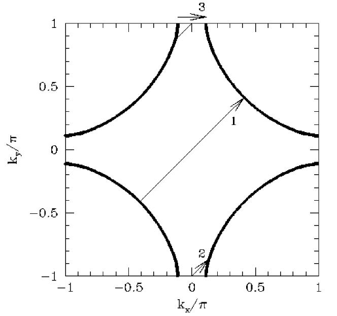
Figure 7: Fermi surface of a tight-binding band with near- and next-near-hopping, Eq. (28), with $t^{\prime}/t=-0.3$ and $\mu/t=-1.0$.

The Fermi surface for $t^{\prime}/t=-0.3$ and $\mu/t=-1.0$ is shown in Fig. 7. Results of a numerical calculation for $Im\,\Lambda\,(q,\omega)/\pi$ for this case are plotted in Figs. 8(a) and 8(b) for $q_{y}=0$ and $q_{x}=q_{y}$, respectively. For $q_{y}=0$, the nesting vector 3 is shown in Fig. 7. If we consider the closed Fermi surface around $(\pi,\pi)$, one can see that the two points of this closed Fermi surface that are connected by the wave vector labeled 3, have $\Delta q$ greater than $\pi$. In fact, $\Delta q/\pi\simeq 1.76$, so that when this is folded back into the first Brillouin zone, the cusp occurs at $\Delta q/\pi\simeq-.24$. Also, as we saw previously in Fig. 6(a) the cusp rises from smaller values of $q$ in the reduced zone although in an extended zone scheme it would be approached from larger $q$ values just as in the free electron case. The peaks in the response for $q_{x}=q_{y}$ shown in Fig. 8(b) arise from the nesting vectors labeled 1 and 2 in Fig. 7.

To conclude this Section on the normal state, we consider an electron-phonon system with a self-energy $\Sigma(\omega)$ which depends only upon the frequency. In this case, the momentum that enters the Hankel function giving $G(x,\omega)$ is

$$k(\omega)\cong k_{F}+\frac{(\omega-\Sigma(\omega)}{v_{F}}.$$ (29)

The real part of the self-energy leads to a shift in the wave length of the modulations and the imaginary part of $\Sigma$ leads to their exponential decay on a scale $\ell=v_{F}/(-2\Sigma_{2}(\omega))$. This behavior is reflected in a shift in the position and a rounding of the cusp in the power spectrum $P(q,\omega)$. For values of $\omega$ which are small compared to a typical phonon frequency

$$k(\omega)\simeq k_{F}+\frac{(1+\lambda)\omega}{v_{F}}$$ (30)

with $\lambda=2N(0)|g|^{2}/\Omega_{0}$ the dimensionless electron phonon interaction strength. Here $g$ is the effective electron-phonon coupling and $\Omega_{0}$ a typical phonon energy. As $\omega$ increases $2k_{F}(\omega)$ will reflect the detailed dependence of both the real and imaginary parts of $\Sigma(\omega)$.

III The FT-STM Power Spectrum of a Superconductor

Next consider the case of a superconductor. Here, for an on-site energy perturbation, we have BFS93

$$\delta N(x,\omega)=-\frac{1}{\pi}\ Im\,\int d^{2}{x^{\prime}}\left(G\left(x-x^{\prime},\omega\right)G\left(x^{\prime}-x,\omega\right)-F\left(x-x^{\prime},\omega\right)F\left(x^{\prime}-x,\omega\right)\right)\delta\epsilon\left(x^{\prime}\right)$$ (31)

with $G(x,\omega)$ the usual single particle propagator

$$G(x,\omega)=\int\frac{d^{2}k}{(2\pi)^{2}}\,e^{ik\cdot x}\,\frac{\omega+\epsilon_{k}}{\omega^{2}-\epsilon^{2}_{k}-\Delta^{2}_{k}+i\delta}$$ (32)

and $F(x,\omega)$ the anomalous Gor’kov propagator

$$F(x,\omega)=\int\frac{d^{2}k}{(2\pi)^{2}}\,e^{ik\cdot x}\,\frac{\Delta_{k}}{\omega^{2}-\epsilon^{2}_{k}-\Delta^{2}_{k}+i\delta}.$$ (33)

In this case ref2

$$\Lambda\,(q,\omega)=\int\frac{d^{2}k}{(2\pi)^{2}}\biggl{(}G(k+q,\omega)\,G(k,\omega)-F\,(k+q,\omega)F\,(k,\omega)\biggr{)}$$ (34)

For a 2D $s$-wave superconductor with $\Delta_{k}=\Delta$ and $\epsilon_{k}=k^{2}/2m-\mu$, these Green’s functions have characteristic wave vectors

$$k_{\pm}(\omega)=k_{F}\left[1\pm\frac{\sqrt{\omega^{2}-\Delta^{2}}}{\mu}\right]^{\frac{1}{2}}$$ (35)

The wave length of the ripples in $\delta N(x,\omega)$ are set by $2k_{\pm}(\omega)$. For $\omega<\Delta$, the ripples exponentially decay. If the impurity perturbation involved a change in the size of the gap, there would be a quasi-particle interference contribution involving $k_{+}(\omega)-k_{-}(\omega)=2k_{F}\sqrt{\omega^{2}-\Delta^{2}}/\mu$. The ripples associated with this contribution vary on a length scale set by $v_{F}/\Delta$ which is of order the coherence length rather than $k_{F}^{-1}$. It is this type of spatial oscillation that is responsible for the Tomasch oscillations Tom65 . While Tomasch ripples at $Q_{T}(\omega)=k_{+}(\omega)-k_{-}(\omega)$ are not present for the case of a charge impurity in an isotropic $s$-wave superconductor, they can appear for a $d$-wave superconductor as discussed below.

As shown in Appendix B, it is straightforward to evaluate $Im\,\Lambda\,(q,\omega)$ for an $s$-wave BCS superconductor and one finds that

$$\frac{1}{\pi}\,Im\,\Lambda\,(q,\omega)=4\pi\,N^{2}(0)\ \left(\frac{\omega-\sqrt{\omega^{2}-\Delta^{2}}}{\sqrt{\omega^{2}-\Delta^{2}}}\right)\ \frac{1}{q}\ \frac{1}{\sqrt{q^{2}-4k^{2}_{-}(\omega)}}$$ (36)

for $2k_{-}(\omega)<q<2k_{+}(\omega)$ and

$$\frac{1}{\pi}\,Im\,\Lambda\,(q,\omega) = 4\pi\,N^{2}(0)\left(\frac{\omega-\sqrt{\omega^{2}-\Delta^{2}}}{\sqrt{\omega^{2}-\Delta^{2}}}\right)\ \frac{1}{q}\ \frac{1}{\sqrt{q^{2}-4k^{2}_{-}(\omega)}}$$ (37)

$$+ 4\pi\,N^{2}(0)\left(\frac{\omega+\sqrt{\omega^{2}-\Delta^{2}}}{\sqrt{\omega^{2}-\Delta^{2}}}\right)\ \frac{1}{q}\ \frac{1}{\sqrt{q^{2}-4k^{2}_{+}(\omega)}}$$

for $2k_{+}(\omega)<q$. More generally, for an electron-phonon system the frequency-dependent complex gap $\Delta(\omega)$ would replace $\Delta$. Normalizing by $\sqrt{n_{i}}N(0)\,|\delta\epsilon|/\mu$, as previously done for the free electron case, we have plotted $|\bar{N}(q,\omega)|$ versus $q$ in Fig. 9 for a BCS $s$-wave superconductor with $\Delta/\mu=0.1$. The coherence factors in Eq. (36) and (37) give more weight to the $2k_{+}(\omega)$ cusp for positive values of $\omega$ associated with a bias voltage that probes the empty states, Fig. 9(a), while the $q=2k_{-}(\omega)$ cusp is enhanced when the bias is reversed as shown in Fig. 9(b).

We turn next to the case of a $d$-wave superconductor with

$$\Delta_{k}=\Delta_{0}(\cos k_{x}-\cos k_{y})/2$$ (38)

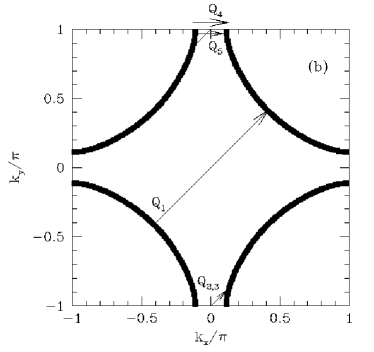
Figure 10: Characteristic wave vectors for a d-wave superconductor with a tight-binding band, Eq. (28), with $t^{\prime}/t=-0.3$, $\mu/t=-1.0$, and $\Delta_{0}=0.1t$. The contours of the solid regions correspond to the points where $\omega=\sqrt{\epsilon_{k}^{2}+\Delta_{k}^{2}}$ with (a) $\omega=0.5\Delta_{0}$, and (b) $\omega=1.1\Delta_{0}$. The dashed line in (a) shows the Fermi surface of the non-interacting system. In (b) $Q_{3}$ and $Q_{5}$ ($Q_{4}$ and $Q_{2}$) connect the innermost (outermost) surfaces while $Q_{1}$ connects the outermost surfaces.

and a bandstructure given by Eq. (28) with $t^{\prime}/t=-0.3$ and $\mu=-1.0$. The Fermi surface for these parameters is shown as a dashed line in Fig. 10(a). The contours of the solid regions correspond to the loci of points where $\omega=\sqrt{\epsilon_{k}^{2}+\Delta_{k}^{2}}$ for $\omega=0.5\Delta_{0}$ in Fig. 10(a) and $\omega=1.1\Delta_{0}$ in Fig.10(b). Results for $|Im\,\Lambda\,(q,\omega)/\pi|$ at various values of $\omega$ less than $\Delta_{0}$ are shown in Fig. 11(a) for $q_{x}=q_{y}$ and Fig. 11(b) for $q_{y}=0$. For the diagonal cut with $q_{x}=q_{y}$, there is a response at the wave vector ${\bf q}_{7}(\omega)$ shown in Fig. 10(a) which connects the end points of the $\omega^{2}=\epsilon^{2}_{k}+\Delta^{2}_{k}$ contour. This peak is similar to the peak we have seen in the case of the ellipse discussed in the previous section. There are two identical contributions coming from the two contours on opposite sides of the Fermi surface. As the bias voltage $eV=\omega$ increases, one sees that $q_{7}(\omega)$ peak moves to larger values of momentum. This reflects the increase in magnitude of the wavevector $q_{7}(\omega)$ as $\omega$ is increased and can provide information on the $k$-dependance of the Fermi surface and gap Hof02 ; McE02 . In addition, there is a contribution coming from ${\bf q}_{3}(\omega)$ which connects the tips of two opposite contours which increases more slowly with $\omega$. Finally, there is a response associated with ${\bf q}^{\prime}$ shown in Fig. 10(a). This is the response due to the wave vector labeled 1 in Fig. 7 and shown in the diagonal $q_{x}=q_{y}$ response of the normal metal with this same bandstructure in Fig. 8(b). Approximate analytic results for the $d$-wave case are given in Appendix B, Eqs. (67) and (70).

Similarly in Fig. 11(b), for $q_{y}=0$ one finds structure associated with the wave vectors ${\bf q}_{1}$ and ${\bf q}_{5}$ shown in Fig. 10(a). As discussed by McElroy et. al, McE02 this structure arises from a peak in the joint density of states associated with the overlap of the ends of two opposite $\omega^{2}=\epsilon^{2}_{k}+\Delta^{2}_{k}$ contours. Just as for the case of the elliptical Fermi surface previously discussed, the strength of the cusp depends upon the curvature of the dispersion. The increase of $q_{1}(\omega)$ with increasing $\omega$ again provides information on the Fermi surface and $\Delta_{k}$. The peak at $q_{5}(\omega)$ initially increases with $\omega$ and would continue to increase in an extended zone but here, for $\omega\gtrsim 0.25$, it is reflected back into the first Brillouin zone. Finally, there is a weak cusp at low momentum $Q_{T}(\omega)$ associated with the Tomasch interference process.

Note that the response seen in $|\bar{N}(q,\omega)|$ associated with quasi-particle interference is actually characterized by a continuous curving cusp in the $(q_{x},q_{y})$ plane whose intensity is related to the joint density of the $k$ and $k+q$ quasi-particle states. When we take into account all four quadrants, the structure in the power spectrum $P(q,\omega)$ in the first Brillonin zone becomes much richer. Not only are there cusps associated with scattering processes confined to similar contour regions in quadrants 2 and 4, which give rise to a cusp whose major axis is perpendicular to that due to quadrants 1 and 3, there are cusps from scattering processes between the four nodal regions. In addition, there is the response associated with the nodal wave vector ${\bf q}^{\prime}$. In order to see this more clearly, we have calculated $\Lambda\,(q,\omega)$ for the case in which $t^{\prime}=0$. In Fig. 12 we compare the results for $|Im\,\Lambda\,(q,\omega)/\pi|$ calculated with $t^{\prime}=0$ [Fig. 12(a)] and with $t^{\prime}/t=-0.3$ [Fig. 12(b)]. In both cases, we clearly see the contributions of ${\bf q}_{3}$ and ${\bf q}_{7}$. In addition, a ${\bf q}^{\prime}$ contribution from the nodal region is also visible. The ${\bf q}_{3}$ contribution is weaker for the case in which $t^{\prime}=0$. In this case we also find that $|{\bf q}_{3}|<|{\bf q}^{\prime}|$ as one can see from the insets in the figures.

When $\omega$ is greater than $\Delta_{0}$, structure in $|N(q,\omega)|$ is associated with the $Q_{\alpha}$ vectors shown in Fig. 10(b), for $\omega=1.1\Delta_{0}$. In this case, for $q_{x}=q_{y}$, $|N(q,\omega)|$ exhibits structure at $q_{x}=Q_{1}$, $Q_{2}$, and $Q_{3}$, see Fig. 13(a). The weak structure at large momentum transfer $Q_{1}$ is similar to the structure for the normal state labeled ”1” in Fig.8, since the gap vanishes along the diagonal. The structures at $Q_{2}$ and $Q_{3}$ correspond to interference processes between the particle like and the hole like BCS quasi particles. Just as for the $s$-wave case, for $\omega>0$, the coherence factor gives more weight to the $Q_{2}$ process. Results for $|N(q,\omega)|$ versus $q_{x}$ for $q_{y}=0$ are shown in Fig. 13(b). In this case, structure appears associated with $q_{x}=Q_{4}$ and $Q_{5}$ with the coherence factors leading to a large response at $Q_{4}$ for positive $\omega$. As noted earlier, in the cuprate superconductors lifetime effects suppress this $\omega>\Delta_{0}$ structure, making it difficult to see in the experimental studies.

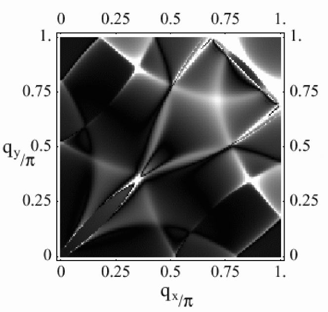
Figure 14: Intensity map of the quasi-particle interference response $|Im\,\Lambda(q,\omega)/\pi|$ for a $d$-wave superconductor plotted over the first $(q_{x},q_{y})$ quadrant. Here, the band structure is given by Eq. (28) with $t^{\prime}/t=0.3$ and $\mu=-1.0$, $\Delta_{k}$ is given by Eq. (38) and the bias is $\omega=0.5\Delta_{0}$.

The structure in the quasi-particle interference response can also be seen in the intensity map plots of $|Im\,\Lambda\,(q,\omega)/\pi|$ over the $(q_{x},q_{y})$ plane. One such map for $\omega=0.5\Delta_{0}$ is shown in Fig. 14. Here one sees that the response is characterized by continuous curving intensity cusps in the $(q_{x},q_{y})$ plane. Like the case of the elliptical Fermi surface, the intensity can have significant variations along the cusps due to the curvature of the quasi-particles dispersion relation. Going out from the origin along $q_{x}=q_{y}$ as in Fig. 12(b), one first sees a bright (high intensity region) cusp associated with $q_{7}$. At large momentum values along this same 45^∘ line one sees a narrow bright line associated with $q^{\prime}$ scattering processes which connect the outter edges of the $\omega=\sqrt{\epsilon^{2}_{k}+\Delta^{2}_{k}}$ envelopes. Finally, the brighter, curved region of intensity near the $(\pi,\pi)$ corner arises from $q_{3}$ interference processes associated with the inner boundaries of these contours. The bright regions near $(q_{x}/\pi=0.85,q_{y}/\pi=0.3)$ and $(q_{x}/\pi=0.3,q_{y}/\pi=0.85)$ arise from interference effects associated with $q_{2}$ and $q_{6}$ of Fig. 10(a).

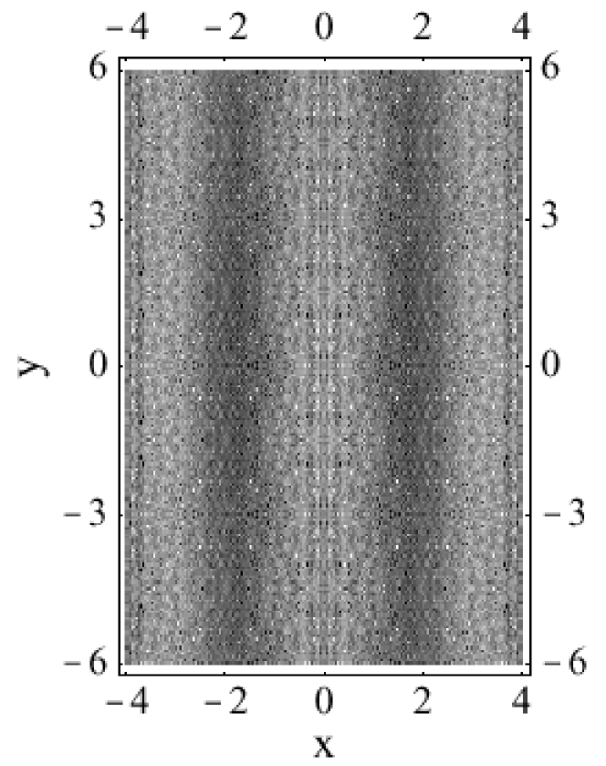
Figure 15: Ripples in $N(x,\omega)$ when there is an ordered array of scattering centers running along the $y$-axis. Here the spacing between the stripes correspond to 4 lattice sites and $\omega=0.5\Delta_{0}$.

Finally, we consider the response of a $d$-wave superconductor when there is an ordered stripe array of weak scattering centers. In Fig. 15 we show the ripples produced in $N(x,\omega)$ when the scattering centers form a stripe-like structure oriented along the $y$-axis with a spacing of four lattice sites. For the parameters we have chosen, $q_{5}(\omega)\simeq\pi/2$ for $\omega=0.5\Delta_{0}$ with $\Delta_{0}$ the maximum value of the $d$-wave gap. As seen in Fig. 15, the ordered array of stripe scattering centers produces an oriented set of ripples. These give rise to the structure in $|N(q,\omega)|$ shown in Fig. 16 for $q\simeq\pi/2$. Here we have assumed that there is quasi-particle scattering from a random array of impurities as well as the stripes. These contributions add incoherently so that

$$\left\langle\left|\delta\epsilon(q)\right|^{2}\right\rangle\sim\left[1+A\frac{\Gamma/\pi}{(q_{x}-Q_{x})^{2}+\Gamma^{2}}\right]~{}.$$ (39)

Here $Q_{x}=\pi/2$ and we have taken $\Gamma=0.01$ and $A=0.5$ in Fig. 16 to illustrate the possible interplay of the scattering from the random impurities and the stripes. The quasi-particle interference peak associated with $q_{1}$ moves to lower values of $q_{x}$ as $\omega$ increases while the response associated with the ordered array of scattering centers remains fixed at $q_{x}\simeq 0.5\pi$ and only its amplitude changes with $\omega$. For larger values of $A$, the stripes would be the dominant feature while for smaller values of $A$ scattering from the random impurities would dominate the power spectrum.

IV Conclusions

Here we have discussed some detailed examples which illustrate what can be learned from FT-STM studies of layered materials. For the case of a weak potential perturbation we have seen that the wave vector power spectrum of the local tunneling density of states, $P(q,\omega)$, contains information on the quasi-particle spectrum and the structure factor of the scatterers. This is also the case for dilute impurities even if they act as strong scattering centers and $\delta\epsilon$ is replaced by a t-matrix. For a normal metal, one can determine information about the nesting properties of the Fermi surface from the loci of the ${\bf q}$-space cusps for $\omega\to 0$. In addition, the dressed Fermi velocity can be obtained from the $\omega$ dependence of the position of the cusp. In fact, from the $\omega$ dependence of the cusp position and its rounding, one can, in principle, obtain information on the real and imaginary parts of the electron self-energy.

In the superconducting state, one can also obtain information on both the wave vector and frequency dependence of the gap $\Delta(k,\omega)$. Again, just as in the case of a normal metal, the signature of these quasi-particle interference effects are continuous “arcs” of cusps in ${\bf q}$-space. However, the intensity variation along the arcs may be large due to changes in the effective density of states associated with a given momentum transfer ${\bf q}$, making the intensity appear more like spots. The rapid change in intensity is due to the small parameter $\Delta_{0}/t$.

In addition to these effects, one can also obtain information on the static structure factor of the scattering potential $\langle|\delta\epsilon_{q}|^{2}\rangle$. As discussed in Appendix A, for the case of a local potential, averaging over a $\Delta q_{x}$ by $\Delta q_{y}$ block of $q$ values about a given $q$ leads to $\langle|\delta\epsilon_{q}|^{2}\rangle/N\simeq n_{i}\delta\epsilon^{2}$. However, if the scattering potential has long-range order, such as is the case for the $BiO_{2}$ over layer in the BISCO studies, one should see a $q$-dependent response in the wave-vector power spectrum of the local tunneling density of states for ${\bf q}$ values equal to the reciprocal lattice vectors of the $BiO_{2}$ layer. This response will be particularly strong for $\omega\simeq\Delta_{0}$. Similarly, it should be possible to see evidence of pinned stripes in the structure factor if they are present How02 .

As discussed in the introduction, we have focused on the case of weak scattering. As noted, in this limit, where the Born approximation is adequate, one has a simple separation of the response into the quasi-particle interference effects which are contained in $\Lambda(q,\omega)$ and the structure factor of the scatterers which is contained in $\langle|\delta\epsilon_{q}|^{2}\rangle$. Of course, many-body interactions will give rise to additional effects. There will be screening, changing $\delta\epsilon_{q}$ to $\delta\epsilon_{q}/\epsilon(q,0)$ where $\epsilon(q,0)$ is the zero frequency dielectric constant Kivup . Furthermore, there will be vertex corrections so that for example, for a strongly-interacting normal system one will have

$$\Lambda(q,\omega)=\int\frac{d^{2}k}{(2\pi)^{2}}\ \Gamma\,(k,q,\omega)\,G(k+q,\omega)\,G(k,\omega)~{},$$ (40)

with $\Gamma(k,q,\omega)$ the elastic vertex for momentum transfer $q$ and zero energy transfer for an incoming particle with momentum $k$ and energy $\omega$. Similar vertex corrections will occur in the superconducting state. In addition, the quasi-particle dispersion relation can be altered by an interaction which breaks the translational symmetry PDDH02 leading to a different $\omega$ dependence of $|N(q,\omega)|$.

Finally, there is the form factor of the tunneling probe. Here we have neglected the momentum dependence of the tunneling matrix element and simply assumed that the conductance map was proportional to the local tunneling density of states $N(x,\omega)$. However, if this is not the case, a tunneling matrix element form factor

$$T(k)=\sum_{l}e^{ik\cdot l}T(l)$$ (41)

will enter so that for a superconductor

$$\Lambda(q,\omega)=\frac{1}{N}\sum_{k}T^{*}(k+q)T(k)\left[G(k+q,\omega)G(k,\omega)-F(k+q,\omega)F(k,\omega)\right]$$ (42)

For example, a tunneling form factor

$$T(k)=(\cos k_{x}-\cos k_{y})$$ (43)

has been suggested for the case of an STM tip on a cuprate superconductor MB01 . However. because the average tunnelling density of states in these STM experiments appears to vary linearly with $V$ at low voltages, we have modeled the tunnelling as a direct process and neglected its momentum dependence.

Appendix A Random Impurity Structure Factor

Suppose we have an $L\times L$ section of a lattice with a concentration of $n_{i}$ impurities per unit area. Assume that if there is an impurity at site $l$ it has a potential $\delta\epsilon(l)=1$, while if there is no impurity at site $l$, $\delta\epsilon(l)=0$. For a given random configuration of $N_{i}$ impurities on $L\times L=N$ sites, corresponding to an area impurity concentration $n_{i}=N_{i}/N$, we have

$$\delta\epsilon(q)=\sum_{l}e^{iq\cdot l}\delta\epsilon(l).$$ (44)

For this configuration of impurities we can define a power spectrum with

$$P(q)=\frac{\left|\delta\epsilon(q)\right|^{2}}{N}$$ (45)

There is of course a peak for $q=0$, where

$$P(0)=\frac{N_{i}^{2}}{N}.$$ (46)

However for other values of $q$, $P(q)$ fluctuates about $n_{i}$. If one were to average $P(q)$ over many realizations of independent impurity configurations ,

$$\left\langle P(q)\right\rangle=n_{i}\ \mbox{for}\ q\neq 0.$$ (47)

However, if we have an $L\times L$ lattice with a fixed configuration of impurities, the power spectrum $P(q)$, given by Eq. (45), will exhibit fluctuations. If we average $P(q)$ over blocks of $q$ of width $(\Delta q_{x},\Delta q_{y})$ about each $q$ we can reduce these fluctuations. Naturally at the same time, the momentum resolution will be reduced. Define a block smoothed $P(q)$ average as follows:

$$\bar{P}(q)=\frac{1}{N(\Delta q_{x},\Delta q_{y})}\sideset{}{{}^{\prime}}{\sum}_{\Delta q_{x},\Delta q_{y}}P(q),$$ (48)

here the prime on the sum indicates that $P(0)$ is replaced with $n_{i}$ so that the $q=0$ peak is not broadened from the smoothing operation. The sum in Eq. (48) is over a set of q-points $(-\Delta q_{x}/2,\Delta q_{x}/2)$ and $(-\Delta q_{y}/2,\Delta q_{y}/2)$ about each $q$. $N(\Delta q_{x},\Delta q_{y})$ is the number of sites in the $\Delta q_{x}$ by $\Delta q_{y}$ block. We expect that the RMS fluctuations of $\bar{P}(q)$ will decrease inversely as the square root of the number of $q$-values in the $\Delta q_{x}$ by $\Delta q_{y}$ block.

For example, consider a lattice with $L=500$ and one configuration of random impurities with $n_{i}=0.01.$ The power spectrum $P(q)$, given by Eq. (45), versus $q_{x}$ for $q_{y}=0$ is shown in Fig. 17(a). Figures 17(b) and 17(c) show similar plots for the smoothed power spectrum $\bar{P}(q)$, given by Eq. (48), for square blocks with $\Delta q_{x}=\Delta q_{y}=2\pi(2d+1)/L$ for $d=5$ and $d=10$ respectively. Figure 17(d) shows $\bar{P}(q)$ for the case in which only $\Delta q_{y}=2\pi(2d+1)/L$ is averaged with $d=10$. The solid line in each of these figures is $n_{i}=0.01$.

It is clear from the results shown in Fig. 17, that one can reduce the fluctuations in the power spectrum by averaging it over a region of q-space surrounding a given q-point. This is of course just complementary to taking the original $L\times L$ spatial lattice, breaking it up into $L_{B}\times L_{B}$ blocks with $L_{B}=2\pi/\Delta q$, constructing the appropriate Fourier transform for each block and then averaging over the blocks. The more blocks one has, the small the RMS fluctuations of the power spectrum of the Fourier transform. Of course, dividing the $L\times L$ system up into more blocks leads to a corresponding decrease in the momentum resolution. The momentum smoothing operation, Eq. (48), is just another way of blocking.

As a further test of these ideas, we calculate the RMS deviation of $\bar{P}(q)$ from $n_{i}$ versus the momentum block size $2d+1$

$$D=\sqrt{\frac{1}{N}\sum_{q\neq 0}\left(\bar{P}(q)-\frac{1}{N}\sum_{q\neq 0}\bar{P}(q)\right)^{2}}.$$ (49)

In Fig. 18 we show that $D$ varies as $(2d+1)^{-1}$ for large $d$ for several different concentrations of impurities. The straight lines on the plot represent the asymptotic behavior in which $D\sim\alpha n_{i}/(2d+1)$ with $\alpha$ of order one.

Finally, we model the behavior of the magnitude of the wave-vector Fourier transform of the local tunneling density of states by

$$\left|N(q)\right|=\sqrt{P(q)}\times\left\{\begin{array}[]{ll}\frac{1}{\sqrt{q-q^{\star}}}&\mbox{if $q>q^{\star}=\pi/4$}\\ 0&\mbox{otherwise}.\end{array}\right.$$ (50)

The results for $L=500$ and $n_{i}=0.01$ are shown in Figs. 19(b)-(c) for the $\mbox{BlockAvg}\left[\left|N(q_{x},q_{y}=0)\right|\right]$, averaged over a $\Delta q_{x}\times\Delta q_{y}$ square with $d=5$ and $d=10$ respectively. Figure 19(a) shows the unaveraged result. Similarly Fig. 19(d) shows the $\mbox{LineAvg}\left[\left|N(q_{x},q_{y}=0)\right|\right]$ versus $q_{x}$ for the case in which we only average over a $q_{y}$ segment of width $\Delta q_{y}=2\pi(2d+1)/L$ with $d=10$. Thus the $q$-averaging brings out the underlying structure of the quasi-particle interference factor.

Finally, we note that even without such block averaging, one is still able to see an image of the quasi-particle interference response in an intensity plot of

$$\left|\bar{N}(q,\omega)\right|=\biggl{|}\frac{1}{\pi}Im\,\Lambda\,(q,\omega)\biggr{|}\ \frac{|\delta\epsilon(q)|}{\sqrt{N}}$$ (51)

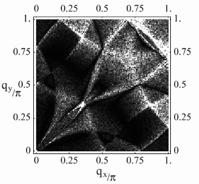
Figure 20: Intensity map of $\left|\bar{N}(q,\omega)\right|$ for the same parameters that were used in Fig. 14. Here $|\delta\epsilon(q)|$ is obtained from Eq. (A1) with one realization of an impurity concentration $n_{i}=0.01$.

over the $(q_{x},q_{y})$ plane. In Fig. 20 we show a plot of $\left|\bar{N}(q,\omega)\right|$ for the same parameters that were used in Fig. 14. Here $|\delta\epsilon(q)|$ is obtained from Eq. (A1) with one realization of an impurity concentration $n_{i}=0.01$. Comparing this figure with Fig. 14, one can see that while the structure is noisy, the key features remain clearly visible.

Appendix B Quasi-particle Interference Response

The quasi-particle interference response function for the 2D free electron gas

$$\frac{1}{\pi}\,Im\,\Lambda(q,\omega)=\frac{1}{\pi}\,Im\,\int\,d^{2}x\,e^{iq\cdot x}G_{o}(x,\omega)\,G_{o}(-x,\omega)$$ (52)

can be directly evaluated using the expression for $G_{o}(x,\omega)$ given by Eq. (15). Since the Hankel function $H^{(1)}_{0}=J_{0}+i\,N_{0}$, we have

$$\frac{1}{\pi}\,Im\,\Lambda\,(q,\omega) = -2\pi\,N^{2}(0)\,\int d^{2}x\,e^{iq\cdot x}J_{0}\,\left(k(\omega)r\right)\,N_{0}\,\left(k(\omega)r\right)$$ (55)

$$= \left\{\begin{array}[]{lccr}8\pi\,N^{2}(0)&\frac{1}{q}&\frac{1}{\sqrt{q^{2}-4k^{2}(\omega)}}&q>2k(\omega)\\ 0&&&q<2k(\omega)\end{array}\right.$$

with $r=|x|$ and

$$k(\omega)=k_{F}\,\left(1+\frac{\omega}{\mu}\right)^{\frac{1}{2}}$$ (56)

We also note that Carrying out the angular integration one has

$$Re\Lambda(q,\omega)=\left\{\begin{array}[]{lr}\frac{8\pi N(0)^{2}}{q^{2}\sqrt{q^{2}-4k^{2}}}\ln\left|\frac{\sqrt{q^{2}-4k^{2}}+1}{\sqrt{q^{2}-4k^{2}}-1}\right|&q>2k(\omega)\\ \qquad\frac{-16\pi N(0)^{2}}{q^{2}\sqrt{4k^{2}-q^{2}}}\tan^{-}1\frac{q}{\sqrt{4k^{2}-q^{2}}}&q<2k(\omega)\end{array}\right.$$ (57)

Plots of the real and imaginary parts of $\Lambda(q\omega)$ are shown in Fig. 21. As noted, in Born approximation one only sees $Im\lambda(q,\omega)$. However, when the scattering is stronger, giving rise to a phase shift, both $Re\lambda(q,\omega)$ and $Im\lambda(q,\omega)$ will be present in the quasi-particle interference response. The imaginary part of $\Lambda$ can also be evaluated by noting that for $\omega>0$,

$$\frac{1}{\pi}\ Im\,\Lambda\,(q,\omega) = \frac{1}{\pi}\ Im\,\int\frac{d^{2}k}{(2\pi)^{2}}\ \frac{1}{\omega-\epsilon_{k+q}+i\delta}\ \frac{1}{\omega-\epsilon_{k}+i\delta}$$ (58)

$$= 2\int\frac{d^{2}k}{(2\pi)^{2}}\ \delta\,(\omega-\epsilon_{k})\ \frac{1}{\epsilon_{k+q}-\epsilon_{k}}$$

Carrying out the angular integration one has

$$\int\limits^{2\pi}_{0}\frac{d\phi}{2\pi}\ \frac{1}{\epsilon_{k+q}-\epsilon_{k}}=\left\{\begin{array}[]{lr}\frac{2m}{\sqrt{q^{4}-4k^{2}q^{2}}}&q^{2}>4k^{2}\\ \qquad 0&q^{2}<4k^{2}\end{array}\right.$$ (59)

so that

$$\frac{1}{\pi}\,Im\,\Lambda\,(q,\omega)=2N(0)\int\limits^{q^{2}/8m-\mu}_{-\mu}d\epsilon_{k}\ \delta(\omega-\epsilon_{k})\ \frac{2m}{\sqrt{q^{4}-4k^{2}q^{2}}}$$ (60)

which gives Eq. (55) since $N(0)=m/2\pi$.

For the electron-phonon case in which the self-energy $\Sigma(\omega)=\Sigma_{1}(\omega)+i\Sigma_{2}(\omega)$ only depends on $\omega$, the angular integral can be evaluated in the same way leading to

$$\frac{1}{\pi}\,Im\,\Lambda\,(q,\omega)=2N(0)\int\limits^{q^{2}/8m-\mu}_{-\mu}d\epsilon_{k}\ \frac{\frac{1}{\pi}\ \Sigma_{2}(\omega)}{\left(\omega-\epsilon_{k}-\Sigma_{1}(\omega)\right)^{2}+\Sigma^{2}_{2}(\omega)}\ \frac{2m}{\sqrt{q^{4}-4k^{2}q^{2}}}.$$ (61)

Here, as usual for the electron-phonon problem we have neglected vertex corrections.

For the case of a superconductor with scattering from a site charge potential

$$\Lambda\,(q,\omega)=\int\,\frac{d^{2}k}{(2\pi)^{2}}\ \frac{(\omega+\epsilon_{k+q})\ (\omega+\epsilon_{k})-\Delta_{k+q}\Delta_{k}}{\left(\omega^{2}-E^{2}_{k}+i\,\delta\right)\ \left(\omega^{2}-E^{2}_{k+q}+i\,\delta\right)}$$ (62)

with $E_{k}=\sqrt{\epsilon^{2}_{k}+\Delta^{2}_{k}}$. For a constant $s$-wave gap $\Delta_{k}=\Delta_{0}$ and

$$\frac{1}{\pi}\ Im\,\Lambda\,(q,\omega)=-\frac{2}{\pi}\,Im\,\int\ \frac{d^{2}k}{(2\pi)^{2}}\ \frac{\omega+\epsilon_{k}}{\omega^{2}-E^{2}_{k}+i\,\delta}\ \frac{1}{\epsilon_{k+q}-\epsilon_{k}}$$ (63)

Making use of Eq. (59), we have

$$\frac{1}{\pi}\ Im\,\Lambda\,(q,\omega)=2N(0)\int\limits^{q^{2}/8m-\mu}_{-\mu}d\epsilon_{k}\,\delta\,\left(\omega^{2}-E^{2}_{k}\right)\ \frac{2m}{\sqrt{q^{4}-4k^{2}q^{2}}}\ (\omega+\epsilon_{k}).$$ (64)

Carrying out the $\epsilon_{k}$ integration leads to the results given by Eqs. (36) - (37) in the text.

For a $d$-wave superconductor, we have

$$\frac{1}{\pi}\ Im\,\Lambda\,(q,\omega)=2\int\frac{dk^{2}}{(2\pi)^{2}}\ \delta\,(\omega-E_{k})\ \frac{1}{2E_{k}}\ \frac{(\omega+\epsilon_{k})\ (\omega+\epsilon_{k+q})-\Delta_{k}\Delta_{k+q}}{E^{2}_{k+q}-E^{2}_{k}}.$$ (65)

This integral can be approximately evaluated when $\omega<\Delta_{0}$ for the case in which $\epsilon_{k}=k^{2}/2m-k^{2}_{F}/2m$ and $\Delta_{k}=\Delta_{0}\cos(2\theta)$. For example, for ${\bf q}$ along the 45^∘ direction with $q=q_{x}=q_{y}$ and $q\mathrel{\raise 1.29167pt\hbox{$>$\kern-7.5pt\lower 4.30554pt\hbox{$\sim$}}}k_{F}\omega/\Delta_{0}$, one finds that

$$\frac{1}{\pi}\ Im\,\Lambda\,(q,\omega)\simeq N^{2}(0)\left(\frac{1}{N(0)\Delta_{0}}\right)\ \frac{1}{k_{F}\sqrt{q}}\ \frac{1}{\sqrt{q-\frac{k_{F}\omega}{\Delta_{0}}}}$$ (66)

This corresponds to the contribution which comes from a momentum transfer that connects the ends of one $\omega=\sqrt{\epsilon_{k}^{2}+\Delta^{2}_{k}}$ contour (i.e. a ${\bf q}_{7}(\omega)$ wave vector) similar to the case of the ellipse discussed in Section III. The enhancement factor $(N(0)\Delta_{0})^{-1}$ arises from the large curvature and resulting large density of states at the contours ends.

Keeping $q$ along the 45^∘ diagonal where $q=q_{x}=q_{y}$, there are additional square root peaks in $Im\,\Lambda(q,\omega)/\pi$ which arise when ${\bf q}$ connects two different contours. There is a ${\bf q}_{3}(\omega)$-like peak near which

$$\frac{1}{\pi}\,Im\,\Lambda(q,\omega)\simeq\frac{4\pi\,N^{2}(0)}{q}\ \left(\frac{\omega}{2\Delta_{0}}\right)\ \frac{1}{\sqrt{k_{F}-q}}\ \frac{1}{\sqrt{{\bf q}_{3}(\omega)-q}}$$ (67)

when

$$q<q_{3}(\omega)=2k_{F}\left(1-\frac{1}{2}\ \left(\frac{\omega}{2\Delta_{0}}\right)^{2}\right).$$ (68)

There is also a peak associated with

$$q^{\prime}(\omega)=2k_{F}\left(1+\frac{\omega}{\mu}\right)^{\frac{1}{2}}$$ (69)

where

$$\frac{1}{\pi}\,Im\,\Lambda(q,\omega)\simeq\frac{4\pi\,N^{2}(0)}{q}\ \left(\frac{\omega}{2\Delta_{0}}\right)\ \frac{1}{\sqrt{q-q^{\prime}(\omega)}}\ \frac{1}{\sqrt{q-q_{3}(\omega)}}$$ (70)

when $q>q^{\prime}(\omega)$. In the limit $\Delta_{0}\to 0$, this last expression becomes

$$\frac{1}{\pi}\,Im\,\Lambda(q,\omega)\simeq\frac{4\pi\,N^{2}(0)}{q\sqrt{k_{F}}\ \sqrt{q-2k(\omega)}}$$ (71)

which is the free electron result Eq. (55) for $\omega/\mu\ll 1$.

  

  

Figure 2: Plot of the normalized $|N(q,\omega)|$ versus $q$ for a free electron gas for various values of $\omega/\mu$.

Figure 3: Plot of the normalized mean-free path corrected $|N(q,\omega)|$ versus $q$ for an electron gas with $\omega=0$. Here $\Gamma=(\ell\,k_{F})^{-1}$: $\Gamma=0$ (solid), $\Gamma=0.01$ (long dashed), $\Gamma=0.05$ (dashed), $\Gamma=0.1$ (dotted).

Figure 4: Plot of the normalized $|N(q,\omega)|$ versus $q$, Eq. (24), for an elliptical Fermi surface with $\gamma^{2}=m_{x}/m_{y}=9$ and $\omega=0$. In (a) $q_{x}=0$ and in (b) $q_{y}=0$

Figure 6: $|Im\,\Lambda(q,\omega)/\pi|$ for the tight-binding band, Eq. 25, with $t=1$ versus $q$ for $\omega=0$ and (a) the diagonal cut-a and (b) the horizontal cut-b indicated in Fig. 5. The dashed curves show the results in the second Brillouin zone. For the cut-a, $2k_{F}^{xy}\simeq.8\pi$ so the solid curve in the first Brillouin looks similar to the free electron response. However, for cut-b, $2k_{F}^{x}\simeq 1.3\pi$ so that the dashed curve in (b) looks similar to the free electron response and the solid curve in the first Brilloin zone results from folding the dashed curve back into the first zone.

Figure 8: $|Im\,\Lambda(q,\omega)/\pi|$ versus $q$ for $\omega=0$ for the tight-binding Fermi surface shown in Fig. 7. (a) $q_{y}=0$ and (b) $q_{x}=q_{y}$.

Figure 9: Plot of the normalized $|N(q,\omega)|$ versus $q$ for an $s$-wave superconductor with a cylindrical Fermi surface and $\Delta/\mu=0.5$. (a) Results for positive values of $\omega=eV$ and (b) for negative values of $\omega$.

Figure 11: $|Im\,\Lambda(q,\omega)/\pi|$ versus $q$ for a $d$-wave superconductor with a tight-binding band given by Eq. (28) with $t^{\prime}/t=-0.3$, $\mu/t=-1.0$, $\Delta_{0}=0.1t$. Here (a) shows results for a diagonal cut for $q_{x}=q_{y}$ and (b) shows results for a horizontal $q_{y}=0$ cut. The $q_{\alpha}$ and $q^{\prime}$ vectors are shown in Fig 10(a).

Figure 12: $|Im\,\Lambda(q,\omega)/\pi|$ versus $q$ for a diagonal cut in which $q_{x}=q_{y}$. (a) shows results for a tight-binding band with $t^{\prime}/t=0$ and (b) shows results for $t^{\prime}/t=-0.3$. $\omega=0.5\Delta_{0}$ and the other parameters are the same of Fig. 11.

Figure 13: $|Im\,\Lambda(q,\omega)/\pi|$ versus $q$ for a $d$-wave superconductor with a tight-binding band given by Eq. (28) with $t^{\prime}/t=-0.3$, $\mu/t=-1.0$, $\Delta_{0}=0.1t$, and $\omega=1.1\Delta_{0}$. Here (a) shows results for a diagonal 45^∘ cut for $q_{x}=q_{y}$ and (b) shows results for a horizontal $q_{y}=0$ cut. The $Q_{\alpha}$ vectors are shown in Fig 10(b).

Figure 16: Structure in $\left|\bar{N}(q,\omega)\right|$ versus $q_{x}$ for random impurities and an ordered array of stripes separated by 4 lattice spacings. The quasi-particle interference peaks associated with $q_{1}(\omega)$ and $q_{5}(\omega)$, previously shown in Fig. 11(b), are seen along with a peak at $q\simeq 0.5\pi$ which arises from the striped array of scattering centers.

Figure 17: Power spectrum, as defined in Eq. (45) for a random configuration of impurities with concentration $n_{i}=0.01$. Here (a) shows the unaveraged results, (b) and (c) show the average over blocks of size $\Delta q_{x}=\Delta q_{y}=2\pi(2d+1)/L$ with $d=5$ and $d=10$ respectively, and (d) shows the average over lines of length $\Delta q_{y}=2\pi(2d+1)$ with $d=10$.

Figure 18: RMS deviation of $\bar{P}(q)$ from $n_{i}$ as defined in Eq. (49). The straight lines represent the asymptotic behavior in which $D\sim\alpha n_{i}/(2d+1)$.

Figure 19: The magnitude of the Fourier transform of the local tunneling density of states, as defined in Eq. (50) for a random configuration of impurities with concentration $n_{i}=0.01$. Here (a) shows the unaveraged results, (b) and (c) show the average over blocks of size $\Delta q_{x}=\Delta q_{y}=2\pi(2d+1)/L$ with $d=5$ and $d=10$ respectively, and (d) shows the average over lines of length $\Delta q_{y}=2\pi(2d+1)$ with $d=10$.

Figure 21: The real (solid) and imaginary (dashed) part of the quasi-particle interference response versus $q$ for a non-interacting 2D electron gas.

- (1) J.E. Hoffman, K. McElroy, D.-H. Lee, K.M. Lang, H. Eisaki, S. Uchida, and J.C. Davis, Science, 295, 466 (2002).
- (2) C. Howald, H. Eisaki, N. Kaneko, and A. Kapitulnik, e.print cond-mat/0201546.
- (3) K. McElroy, R.W. Simmonds, J.E. Hoffman, D.-H. Lee, J. Orenstein, H. Eisaki, S. Uchida, and J.C. Davis, to appear in Nature, March 2003.
- (4) J.M. Byers, M.E. Flatté, and D.J. Scalapino, Phys. Rev. Lett. 71, 3363 (1993).
- (5) There have been various discussions of the effect of the tunneling matrix elements on the relationship between the conductance measured on the layer and the local density of the states of the underlying layer. See for example I. Martin and A.V. Balatsky, Physica C 357–360, 46 (2001). Here, for most of our present discussion, we assume that it is the local density of states at the site that is probed.
- (6) M.E. Flatté and J.M. Byers, Solid State Physics 52, 137 (1999).
- (7) H. Ding, J.C. Campuzano, M. Randeira, A.F. Bellman, T. Yokoya, T. Takahashi, T. Mochiku, and K. Kadowaki, Phys. Rev. B54, R9678 (1996).
- (8) Q.-H. Wang and D.-H. Lee, e.print cond-mat/0205118.
- (9) A calculation of for the free electron case as well as a discussion of screening corrections of the scattering potential are given in S.A. Kivelson, E. Fradkin, V. Oganesyan, I.P. Bindloss, J.M. Tranquada, A. Kapitulnik, and C. Howald, “How to Detect Fluctuating Order in the High Temperature Superconductors”, e. print cond-mat/0210683.
- (10) We thank S. Kivelson for discussing this point with us.
- (11) Here we have considered only scattering by a site charge potential, one could also consider scattering from a variation in the gap or spin degrees of freedom by changing the coherence factors in .
- (12) W.J. Tomasch, Phys. Rev. Lett. 15, 672 (1965).
- (13) D. Podolsky, E. Demler, K. Damle, and B.I. Halperin, e.print cond-mat/0204011; A. Polkovnikov, S. Sachdev, and M. Vojta, cond-mat/0208334.