Quasi-stationary states in low-dimensional Hamiltonian systems

Abstract

We address a simple connection between results of Hamiltonian nonlinear dynamical theory and thermostatistics. Using a properly defined dynamical temperature in low-dimensional symplectic maps, we display and characterize long-standing quasi-stationary states that eventually cross over to a Boltzmann-Gibbs-like regime. As time evolves, the geometrical properties (e.g., fractal dimension) of the phase space change sensibly, and the duration of the anomalous regime diverges with decreasing chaoticity. The scenario that emerges is consistent with the nonextensive statistical mechanics one.

PACS numbers: 05.70.Ln 05.10.-a 05.20.Gg 05.45.Ac

The methods of usual, Boltzmann-Gibbs (BG), statistical mechanics apply to impressively large classes of macroscopic systems. However, the situation is more delicate for complex systems. Indeed, turbulent fluids [1], high-energy collision processes [2], classical [3] and quantum chaos [4], stellar self-gravitating systems [5], granular systems [6], economics [7], motion of micro-organisms [8], and others, frequently exhibit anomalous behaviors where alternative approaches are needed. In particular, in many-body long-range-interacting Hamiltonian systems, it has been recently observed the emergence of long-standing (in the thermodynamical limit infinite-lasting) quasi-stationary (metastable) states (QSS) characterized by non-Gaussian velocity distributions, before the Boltzmann-Gibbs (BG) equilibrium is attained [9, 10]. This is a major concern, as, for these Hamiltonian systems, the foundation of the BG equilibrium thermodynamics is questioned. Using standard results, in this letter we address a simple connection between chaos theory and thermostatistics, and we focus on a paradigmatic dynamical mechanism that produces QSS very similar to those detected in [9, 10]. These QSS are displayed and characterized by means of low-dimensional symplectic maps.

The foundation of the Boltzmann-Gibbs (BG) equilibrium thermodynamics lies on a sufficiently complete and uniform occupation of the system phase space (the finite Lebesgue measure $\Gamma$-space), taking into account symmetry, energy and similar restrictions. The BG equilibrium descends in fact from the equal-a-priori-probability postulate, that characterizes the microcanonical Gibbsian ensemble (see, e.g., [11]). According to this postulate, each equally-sized accessible region of the phase space (under the macroscopic conditions of the system) equally likely contains the microscopic state of the system. As Einstein pointed out in his criticism of the Boltzmann principle $S=k\ln W$ [12], this postulate should not be taken a priori, but rather justified a posteriori by the underlying dynamics. Indeed, if dynamics is sufficiently chaotic, large portion of the phase space are rapidly occupied by the trajectory of the system and the postulate is a very accurate representation of the dynamical behavior, as testifies more than a century of successes of the BG formalism. But there are also many situations where the system displays an intricate dynamical behavior, as it happens for example at the border between regular and chaotic regimes.

At this border, for a large class of Hamiltonian systems, a mechanism based on the KAM theory operates, which we briefly review now. A continuous Hamiltonian system with $n$ degrees of freedom may be written in the form [13]:

$$H=H_{0}(I_{1},...,I_{n})+\epsilon\;V(I_{1},\theta_{1},...,I_{n},\theta_{n}),$$ (1)

where $H_{0}$ is integrable ($I_{1},...,I_{n}$ are its integrals of motion), $\epsilon<<1$, and $V$ is a nonlinear perturbation. Under certain hypothesis (see, e.g., [13]), for $\epsilon=0$ the trajectories lie on invariant $n$-dimensional tori. A special subset of these tori are called resonance tori. Specifically, if we introduce the (non-degenerate) frequencies of the unperturbed motion: $\omega_{j}\equiv\frac{\partial H_{0}}{\partial I_{j}}\;(j=1,...,n)$, we have that the condition $\sum_{j=1}^{n}m_{j}\omega_{j}=0$ (where $m_{j}$ are integer numbers) defines the resonance tori. Each resonance torus involves the formation of a separatrix loop. The action of the perturbation, for small enough $\epsilon\neq 0$, deforms normal tori into KAM-tori, and, in correspondence with the resonance tori, destroys the separatrices replacing them with stochastic layers. Resonance tori, in the space spanned by $\omega_{1},..,\omega_{n}$, lie in the intersection between the hyperplane defined by the resonance condition and the hypersurface of energy $E=H_{0}(\omega_{1},...,\omega_{n})$. In the case $n>2$, resonance tori must, for topological reasons, intersect between them. Consequently, while for $n\leq 2$ the stochastic layers are distinct for $\epsilon$ sufficiently small, for $n>2$ they merge into a single connected stochastic web that is dense in the phase space for all $\epsilon\neq 0$, and there is room for Arnold diffusion processes. We remark that, for $n=2$, KAM-tori constitute total barriers for diffusive processes in the phase space; nevertheless, inside the stochastic sea, it is possible to find Cantor sets, named cantori, that constitute partial barriers for diffusion (see [14] for details).

A convenient way of studying Hamiltonian systems is by using symplectic maps. A $(2n-2)$-dimensional symplectic map is obtained from conservative Hamiltonian systems with $n$ degrees of freedom by taking a Poincaré section over the hypersurface of constant energy. Interestingly enough, a $2n$-dimensional symplectic map is also the result of a Poincaré section on the phase space of an open system of $n$ degrees of freedom with a Hamiltonian that depends periodically on time. We remark that in both cases the map has a symplectic structure; this assures (hyper)volume conservation in the phase space. The advantage of maps lies on the reduced dimension of the phase space and on the use of a discrete time. In this letter we specifically address some symplectic (hence conservative) maps in order to discuss how equilibrium and quasi-equilibrium can be attained in phase space.

Let us start through the analysis of a prototypical $2$-dimensional symplectic map ($n\leq 2$), the standard (or kicked rotor) map

$$\theta(t+1) = p(t)+\frac{a}{2\pi}\sin[2\pi\theta(t)]+\theta(t)~{}~{}~{}\rm{(mod\;1)},$$ (2)

$$p(t+1) = p(t)+\frac{a}{2\pi}\sin[2\pi\theta(t)]~{}~{}~{}~{}~{}~{}~{}~{}~{}\rm{(mod\;1)}$$

$(a\in{\mathbb{R}},\;\;t=0,1,...)$. $2\pi p$ may be regarded as an angular momentum variable. Notice that, consistently with our scope, we have used the symmetry properties of the map and defined, as usually, the angular momentum $\rm{mod\;1}$. The standard map is integrable for $a=0$, while chaoticity rapidly increases with $|a|$.

In [9, 10], the emergence of the dynamical QSS appeared to be dependent on the initial conditions. Specifically, it was shown that for some classical long-range-interacting $N$-rotor Hamiltonian models, a basin of attraction of initial data exist for which the system dynamically evolves into a QSS whose duration diverges as $N\to\infty$. Typical examples of this basin of attraction are out-of-equilibrium initial conditions called ‘water bag’ initial conditions, characterized by a uniform initial distribution of the angular momenta around zero (see [9, 10] for details). In the case of the standard map, we first observe that the points $(0,1/2)$ and $(1/2,1/2)$ are a $2$-cycle for all $a$ so that we can use them as referential for studying the properties of the phase space with respect to variation of the parameter $a$. With some analogy with [9, 10], our out-of-equilibrium ‘water bag’ initial conditions are defined by considering at $t=0$ a statistical ensemble of $M$ copies of the standard map with arbitrary $\theta$ and $p$ randomly distributed in a small region around $p=1/2$. In standard statistical mechanics, when dealing with systems with diagonal kinetic matrix and zero average momentum, the temperature is proportional to the average square momentum per particle. As we analyze situations with nonzero ‘bulk’ motion, the analogous concept, which we shall refer to as (dimensionless) ‘dynamical temperature’, can be defined as the variance of the angular momentum: $T\equiv\langle(p-\langle p\rangle)^{2}\rangle=\langle p^{2}\rangle-\langle p\rangle^{2}$, where $\langle\rangle$ means ensemble average. The temperature associated with the uniform ensemble (that we will call BG temperature because of its similarity with the equal-a-priori-probability postulate) is given by $T_{\rm{BG}}\equiv\int_{0}^{1}dp\;p^{2}-\left(\int_{0}^{1}dp\;p\right)^{2}=1/12$. It should be noticed that in the present conservative model, the ‘temperature’ $T$ is necessarily bounded since $p$ itself is bounded, in contrast with a true thermodynamical temperature, which is of course unbounded. For large values of $|a|$ (i.e., strong chaoticity) in map (2), the temperature of the ‘water bag’ initial ensemble rapidly relaxes to $T_{\rm{BG}}$ (let us stress that the subindex $BG$ stands for the fact that it corresponds to uniform occupation of the accessible phase space of the map, to be distinguished from the phase space of the physical kicked rotor from which the map was originally deduced). Our aim is to study what happens in the transition to regularity obtained reducing the value of $|a|$ towards $a=0$. In Fig. 1(a) we see that the first effect of the reduction of $|a|$ is that $\lim_{t\to\infty}T(t)<T_{\rm{BG}}$. This is easily understood as follows. As chaoticity reduces, total barriers (KAM-tori) appear in the phase space. As a consequence, the points of the ensemble are prevented to reach all the regions of the phase space and the projection of the ensemble on the $p$ axis produces a probability distribution function (PDF) with a variance smaller than the one of the uniform distribution. For values of $a$ of order $a\sim 1$, a QSS emerges before the relaxation to the final temperature. In fact, inside the stochastic sea partial barriers (cantori) begins to appear, and the initial ‘water bag’ first rapidly diffuse inside an area delimited by cantori and then slowly crosses over to the final relaxation temperature. Fig. 1(c) illustrates this behavior. To obtain a quantitative description of the relaxation time we have plotted the iteration time in a logarithmic scale. We define the crossover time $t_{c}$ as the inflection point of the curve and we observe that it diverges, as $a$ tends to $a_{c}=0.971635406...$ from above, like $t_{c}\sim 1/(a-a_{c})^{2.7}$ (see Fig. 1(b)). Just below this critical value in fact, the strongest cantori close [14], and the relaxation to a higher temperature is prevented. Reducing $a$ to smaller values causes the formation of more and more total barriers, so that the ‘dynamical temperature’ tends to zero for $|a|\to 0$. ¿From the mechanism we have displayed, it is clear that it is possible to obtain these types of QSS even with other sets of initial conditions. Typically, it is sufficient to have the initial data localized inside the first partial barriers. In other words there is an entire basin of attraction of out-of-equilibrium initial conditions that leads to the formation of a certain kind of QSS.

As we pointed out previously, the topology of the phase space changes dramatically for $n>2$. To address this case, we move next to a $4$-dimensional symplectic map composed by two coupled standard maps:

$$\theta_{1}(t+1) = p_{1}(t+1)+\theta_{1}(t)+b\;p_{2}(t+1),$$

$$p_{1}(t+1) = p_{1}(t)+\frac{a_{1}}{2\pi}\sin[2\pi\theta_{1}(t)],$$ (3)

$$\theta_{2}(t+1) = p_{2}(t+1)+\theta_{2}(t)+b\;p_{1}(t+1),$$

$$p_{2}(t+1) = p_{2}(t)+\frac{a_{2}}{2\pi}\sin[2\pi\theta_{2}(t)],$$

where $a_{1},a_{2},b\in{\mathbb{R}},\;t=0,1,...$, and all variables are defined $\rm{mod\;1}$. If the coupling constant $b$ vanishes the two standard maps decouple; if $b=2$ the points $(0,1/2,0,1/2)$ and $(1/2,1/2,1/2,1/2)$ are a $2$-cycle for all $(a_{1},a_{2})$, hence we preserve in phase space the same referential that we had for a single standard map. For a generic value of $b$, all relevant present results remain qualitatively the same. Also, we set $a_{1}=a_{2}\equiv\tilde{a}$ so that the system is invariant under permutation $1\leftrightarrow 2$. Since we have two rotors now, the ‘dynamical temperature’ is naturally given by $T\equiv\frac{1}{2}\left(<p_{1}^{2}>+<p_{2}^{2}>-<p_{1}>^{2}-<p_{2}>^{2}\right)$, hence the BG temperature remains $T_{\rm{BG}}\equiv 1/12$.

As before we consider ‘water bag’ initial conditions, i.e., an ensemble of $M$ points with arbitrary $(\theta_{1}$, $\theta_{2})$, and angular momenta randomly distributed inside a small region around $p_{1}=p_{2}=1/2$. The result is qualitatively similar to the one displayed in Fig. 1(a) for $a>a_{c}$. Large values of $\tilde{a}$ correspond to $T_{{\rm BG}}$ and reducing $\tilde{a}$ we observe the formation of a QSS that, after some time, relaxes to a temperature $T<T_{{\rm BG}}$. The first major difference with the 2-dimensional case is that, because of the Arnold diffusion processes, the relaxation to a higher temperature occurs (waiting enough time) for all $\tilde{a}\neq 0$ (i.e., $\tilde{a}_{c}=0$, defining $\tilde{a}_{c}$ as the value where $t_{c}$ diverges). Moreover, the reason why the ensemble does not relax to the BG temperature for small values of $\tilde{a}$ is here quite different from that for the $2$-dimensional case. Indeed, with this choice of initial data, the initial ‘water bag’ intersects at least a macroscopic island, as clearly appreciated in Fig. 2 (a1); the points that are set inside the island do not diffuse to the outside. As a result, the projection of the ensemble on the plane $p_{1},p_{2}$ conserve a denser central part for all times (Fig. 2 (b1), (c1)).

If we instead shift the initial ‘water bag’, say towards the lower part of the phase space, we can set the points outside this island (Fig. 2 (a2)-(c2)). In this case we obtain a crucial qualitatively new phenomenon, namely the formation, for small values of $\tilde{a}$, of a QSS that eventually relaxes to the BG temperature (see Fig. 3(a)). Notice also that the crossover time $t_{c}$ diverges, as $\tilde{a}\to 0$, faster than in the $2$-dimensional case: $t_{c}\sim 1/\tilde{a}^{5.2}$ (see Fig. 3(b)). We remark that the relaxation to the BG temperature occurs here even if the presence of islands in the phase space violate the equal a priori postulate. In other words, it is possible to obtain a weak violation of the postulate that does preserve a uniform distribution once the ensemble is projected over the plane $p_{1},p_{2}$, in the same sense that a sponge projects a uniform shadow on a wall. These QSS can in fact be geometrically characterized by the fractal dimension $d_{f}$. Overcoming some numerical difficulties involved in a fractal analysis in $4$ dimensions, we illustrate what happens in Fig. 3(c), constructed using a box-counting algorithm [15] (in fact, the phase space exhibits strong inhomogeneities which suggest a multifractal structure). During the QSS the ensemble is, for small $\tilde{a}$, associated with a nontrivial fractal dimension $d_{f}\simeq 2.7$, while, once it crosses over to the BG-like regime, it distributes itself occupying the full dimensionality of the phase space, thus attaining $d_{f}=4$.

These simple models allows also for the discussion of different types of QSS. For instance, at $t=0$ we can set up ‘double water bag’ initial conditions considering an ensemble of $M$ copies of two coupled standard maps with arbitrary $\theta_{1},\theta_{2}$ and angular momenta randomly distributed inside two small regions: $p_{1},p_{2}=0+\delta$ and $p_{1},p_{2}=1-\delta$ ($0<\delta<<1$). In this case, the initial temperature $T(0)$ is higher than $T_{\rm{BG}}$, because the PDFs projected on the $p_{1},p_{2}$ axes are double peaked. Relaxation to $T_{\rm{BG}}$ occurs then from above, as can be seen in Fig. 4. This is precisely in what the phenomenon observed in [10] differs from the one in [9].

It is relevant to notice that, as a consequence of Arnold diffusion, our results for the $4$-dimensional map capture the qualitative behavior of higher-dimension symplectic maps. In fact, the two-plateaux structure has been confirmed by numerical analyses where hundreds of standard maps are all-with-all coupled as in Eq. (3) [16].

Through the numerical analysis of low-dimensional symplectic maps, we have displayed how complex paradigmatic structures associated with conservative nonlinear dynamics can generate anomalous thermodynamical behavior. Particularly, we have exhibited and studied the emergence, while approaching integrability (i.e., when chaoticity decreases), of QSS suggestively similar to those observed in long-range $N$-body systems [9, 10] ($\tilde{a}$ playing a role analogous to $1/N$). A central result is that, in contrast with what happens for the BG equilibrium, these QSS correspond to a nontrivial fractal dimension. This situation reminds the phase space structure of logistic-like maps at the edge of chaos (also characterized by a nontrivial fractal dimension), where exact analytical connections with the nonextensive statistical mechanics [17] have been established [3].

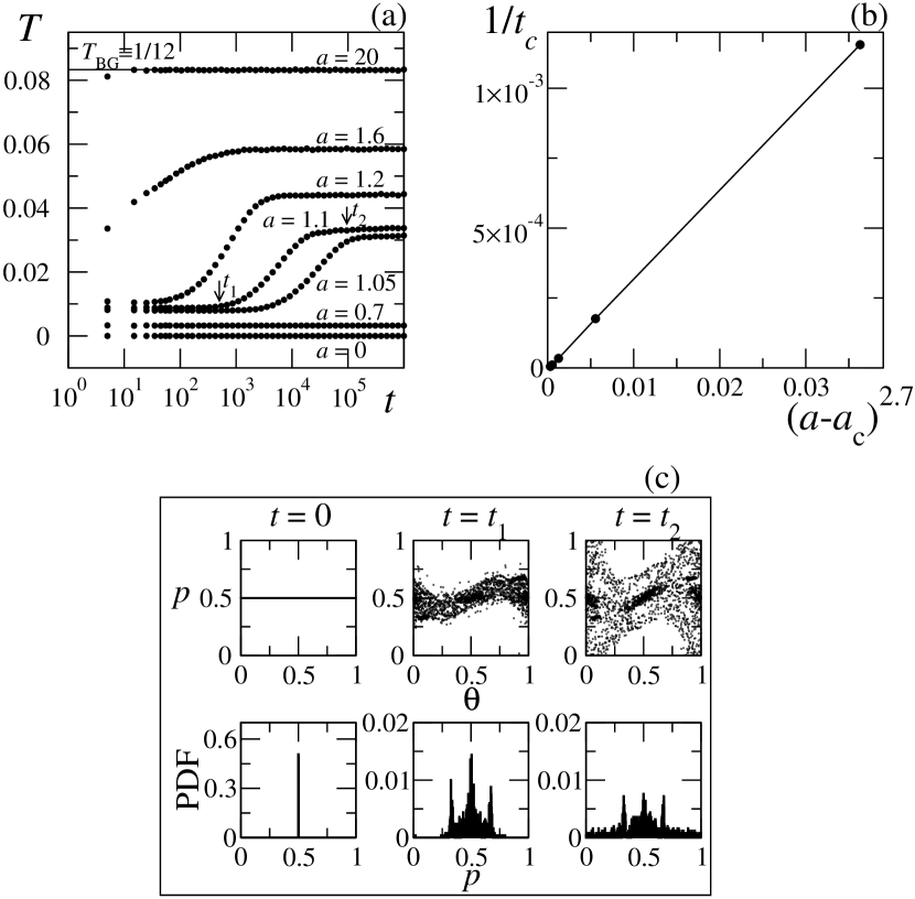
Figure 1: (a) Time evolution of the dynamical temperature $T$ of a standard map, for typical values of $a$. We start with ‘water bag’ initial conditions ($M=2500$ points in $0\leq\theta\leq 1$, $p=0.5\pm 5\;10^{-4}$). In order to eliminate cyclical fluctuations, the dots represent average of $10$ iteration steps; moreover, each curve is the average of $50$ realizations. (b) Inverse crossover time $t_{c}$ (inflection point between the QSS and the BG regimes) vs. $1/(a-a_{c})^{2.7}$. No inflection points subsist if $t$ is linearly represented. (c) Time evolution of the the ensemble in (a) for $a=1.1$ (first row) and PDF of its angular momentum (second row). $t=0$: ‘water bag’ initial conditions; $t=t_{1}=500$: the ensemble is mostly restricted by cantori; $t=t_{2}=10^{5}$: the ensemble is confined inside KAM-tori.

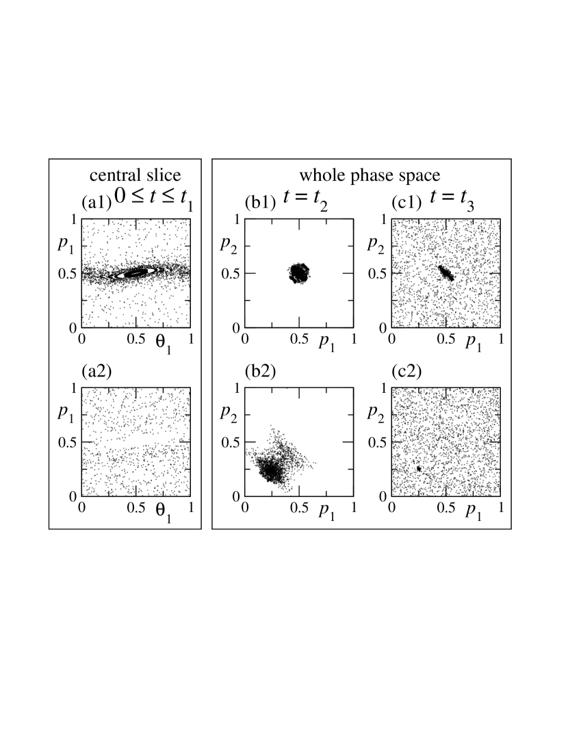
Figure 2: Phase space analysis of the evolution of ‘water bag’ ensembles for two coupled standard maps for $(\tilde{a},b)=(0.4,2)$. First row: ‘Water bag’ initial conditions $0\leq\theta_{1},\theta_{2}\leq 1$, $p_{1},p_{2}=0.5\pm 5\;10^{-3}$. Second row: ‘Water bag’ initial conditions $0\leq\theta_{1},\theta_{2}\leq 1$, $p_{1},p_{2}=0.25\pm 5\;10^{-3}$. (a) Projection on the $(\theta_{1},p_{1})$-plane of the central slice of the phase space ($\theta_{2},p_{2}=0.5\pm 10^{-2}$), for the orbit $0\leq t\leq t_{1}=10^{4}$. (c),(c) Projection on the $(p_{1},p_{2})$-plane of whole phase space for the iterate at time $t_{2}=15$ and $t_{3}=2\;10^{4}$.

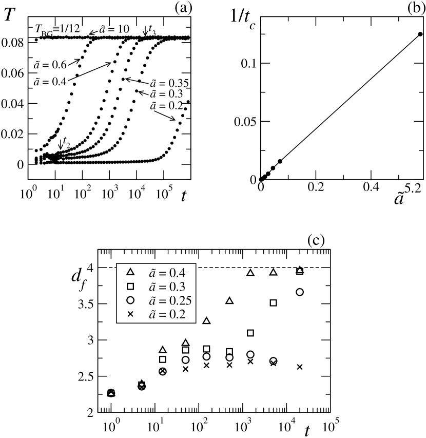
Figure 3: (a) Time evolution of the dynamical temperature $T$ of two coupled standard maps, for $b=2$ and typical values of $\tilde{a}$. We start with water bag initial conditions ($M=1296$ points with $0\leq\theta_{1},\theta_{2}\leq 1$, and $p_{1},p_{2}=0.25\pm 5\;10^{-3}$); moreover, an average was taken over $35$ realizations. See Fig. 2 for $t_{2}$ and $t_{3}$. (b) Inverse crossover time $t_{c}$ vs. $1/\tilde{a}^{5.2}$. (c) Time evolution of the fractal dimension of a single initial ensemble in the same setup of (a).

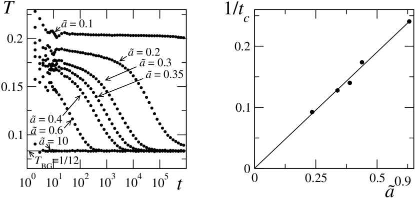
Figure 4: Same as Fig. 3(a),(b) but with ‘double water bag’ initial conditions: $0\leq\theta_{1},\theta_{2}\leq 1$; $p_{1},p_{2}$ randomly distributed inside one of the two regions $p_{1},p_{2}=0+10^{-2}$, $p_{1},p_{2}=1-10^{-2}$.

References

- [1] C. Beck, G.S. Lewis and H.L. Swinney, Phys. Rev. E 63, 035303 (2001); C. Beck, Phys. Rev. Lett. 87, 180601 (2001); T. Arimitsu and N. Arimitsu, Physica A 305, 218 (2002).
- [2] I. Bediaga, E.M.F. Curado and J. Miranda, Physica A 286, 156 (2000); C. Beck, Physica A 286, 164 (2000).
- [3] F. Baldovin and A. Robledo, Phys. Rev. E 66, 045104(R) (2002); F. Baldovin and A. Robledo, Europhys. Lett. 60, 518 (2002); F. Baldovin and A. Robledo, cond-mat/0304410.
- [4] Y.S. Weinstein, S. Lloyd and C. Tsallis, Phys. Rev. Lett. 89, 214101 (2002);
- [5] A. Taruya and M. Sakagami, Phys. Rev. Lett. 90, 181101 (2003).
- [6] S. Gheorghiu, J.R. van Ommen, adn M.-O. Coppens, Phys. Rev. E 67 041305 (2003).
- [7] L. Borland, Phys. Rev. Lett. 89, 098701 (2002).
- [8] A. Upadhyaya, J.-P. Rieu, J.A. Glazier and Y. Sawada, Physica A 293, 549 (2001).
- [9] V. Latora, A. Rapisarda and C. Tsallis, Phys. Rev. E 64, 056134 (2001); A. Campa, A. Giansanti and D. Moroni, Physica A 305, 137 (2002); B.J.C. Cabral and C. Tsallis, Phys. Rev. E 66, 065101(R) (2002); M.A. Montemurro, C. Anteneodo and F. Tamarit, Phys. Rev. E 67, 031106 (2003).
- [10] F.D. Nobre and C. Tsallis, Phys. Rev. E 68, 036115 (2003); E.P. Borges, private communication.
- [11] K. Huang, Statistical Mechanics (J. Wiley and Sons, New York, 1987).
- [12] See, e.g., E.G.D. Cohen, Physica A 305, 19 (2002), and references therein.
- [13] G.M. Zaslavsky, R.Z. Sagdeev, D.A. Usikov and A.A. Chernikov, Weak chaos and quasi-regular patterns (Cambridge University Press, Cambridge 1991).
- [14] R.S. Mackay, J.D. Meiss and I.C. Percival, Physica D 13, 55 (1984).
- [15] A. Kruger, Computer Physics Communications, 98, 224 (1996).
- [16] A.P. Majtey, C. Anteneodo, private communication.
- [17] C. Tsallis, J. Stat. Phys 52, 479 (1988); E.M.F. Curado and C. Tsallis, J. Phys. A 24, L69 (1991) [Corrigenda: 24, 3187 (1991) and 25, 1019 (1992)]. For recent reviews see C. Tsallis, A. Rapisarda, V. Latora and F. Baldovin, in Dynamics and Thermodynamics of Systems with Long-Range Interactions, eds. T. Dauxois, S. Ruffo, E. Arimondo and M. Wilkens, Lecture Notes in Physics 602, 140 (Springer, Berlin, 2002), and M. Gell-Mann and C. Tsallis, eds., Nonextensive Entropy - Interdisciplinary Applications (Oxford University Press, 2003), in preparation. See http://tsallis.cat.cbpf.br/biblio.htm for full bibliography.